| Issue |
A&A
Volume 643, November 2020
|
|
|---|---|---|
| Article Number | A118 | |
| Number of page(s) | 12 | |
| Section | Extragalactic astronomy | |
| DOI | https://doi.org/10.1051/0004-6361/202039358 | |
| Published online | 11 November 2020 | |
Properties of self-gravitating quasi-stationary states
1
CREF, Centro Ricerche Enrico Fermi, Via Panisperna 89A, 00184 Roma, Italy
2
Istituto dei Sistemi Complessi, Consiglio Nazionale delle Ricerche, 00185 Roma, Italy
3
Istituto Nazionale Fisica Nucleare, Dipartimento di Fisica, Università “Sapienza”, 00185 Roma, Italy
e-mail: This email address is being protected from spambots. You need JavaScript enabled to view it.
4
Dipartimento di Fisica, Sapienza, Universitá di Roma, Piazzale Aldo Moro 2, 00185 Roma, Italy
Received:
7
September
2020
Accepted:
24
September
2020
Abstract
Initially far out-of-equilibrium, self-gravitating systems form quasi-stationary states (QSS) through a collisionless relaxation dynamics. These may arise from a bottom-up aggregation of structures or in a top-down frame; their quasi-equilibrium properties are well described by the Jeans equation and are not universal. These QSS depend on initial conditions. To understand the origin of such dependence, we present the results of numerical experiments of initially cold and spherical systems characterized by various choices of the spectrum of initial density fluctuations. The amplitude of such fluctuations determines whether the system relaxes in a top-down or bottom-up manner. We find that statistical properties of the resulting QSS mainly depend upon the amount of energy exchanged during the formation process. In particular, in the violent top-down collapses the energy exchange is large and the QSS show an inner core with an almost flat density profile and a quasi Maxwell-Boltzmann (isotropic) velocity distribution, while their outer regions display a density profile ρ(r) ∝ r−α (α > 0) with radially elongated orbits. We show analytically that α = 4, in agreement with numerical experiments. In the less violent bottom-up dynamics, the energy exchange is much smaller, the orbits are less elongated, and 0 < α(r) ≤ 4, where the density profile is well fitted by the Navarro-Frenk-White behavior. Such a dynamical evolution is shown by both nonuniform spherical isolated systems and by halos extracted from cosmological simulations. We consider the relation of these results with the core-cusp problem and conclude that this can be solved naturally if galaxies form through a monolithic collapse.
Key words: methods: numerical / Galaxy: formation / galaxies: halos
© ESO 2020
1. Introduction
Unlike typical short-range interacting systems, which tend to relax to thermodynamical equilibria through collisions, long-range interacting systems are driven to quasi-equilibrium configurations, or quasi-stationary states (QSS), by a mean-field collisionless relaxation dynamics. These QSS are close to virial equilibrium and their lifetime diverges with the number of particles N because of the decreasing effect of two-body encounters (Lynden-Bell 1967; Padmanabhan 1990; Dauxois et al. 2002; Campa et al. 2014; Levin et al. 2014; Capuzzo-Dolcetta 2019). Comprehension of the statistical properties of the QSS requires the understanding of how their dynamics determines the evolution of the system from an out-of-equilibrium condition to a quasi-stationary configuration.
If the long-range force at work is self-gravity, QSS are reached in two different frames, corresponding to that of a finite and isolated system or to that of a system “embedded” in an expanding space, respectively, this latter representing a typical cosmological case. In both cases, depending on the initial conditions (IC), the dynamics may correspond to a top-down monolithic collapse or to a bottom-up aggregation of substructures. In this work we single out the properties of the IC by determining which evolutionary path brings a certain configuration towards a QSS, regardless of whether the system is finite and isolated or embedded in an infinite expanding background.
The top-down monolithic collapse is modeled, in the simplest way, as the progression of a gravitational instability out of the linearity because such a collapse happens when the over-density is such that the self-gravity dominates over the expanding background (Peebles 1980). If the amplitude of a local over-density is large enough then tidal effects of neighboring density perturbations can be neglected and its evolution proceeds, essentially, as that of an isolated perturbation. These are precisely the hypotheses assumed in the nonlinear, gravitational instability model, known as the spherical collapse model, which is analytically solvable and paradigmatic (Sahni & Coles 1995). Indeed, the evolution of an isolated over-density in an expanding background should reproduce, in physical coordinates, that obtained in open boundary conditions without expansion (Joyce & Sylos Labini 2013). The collapse and stabilization of such an over-density has been studied since the first numerical experiments with self-gravitating systems in both isolated and embedded cases (Henon 1964; van Albada 1982; Aarseth et al. 1988; Aguilar & Merritt 1990; Theis & Spurzem 1999; Boily et al. 2002; Roy & Perez 2004; Boily & Athanassoula 2006; Barnes et al. 2009; Joyce et al. 2009; Sylos Labini 2012, 2013a; Worrakitpoonpon 2015; Merritt & Aguilar 1985; Aguilar & Merritt 1990; Theis & Spurzem 1999; Sylos Labini et al. 2015; Benhaiem & Sylos Labini 2015, 2017; Benhaiem et al. 2016; Spera & Capuzzo-Dolcetta 2017).
On the other hand, a QSS can be originated from a bottom-up hierarchical aggregation process, in which smaller substructures merge to form larger and larger systems. If the system is infinite this process continues without ending, while if the system is finite the aggregation eventually halts. Bottom-up structure formation is typical of standard cosmological scenarios, like the cold dark matter (CDM) scenario because of the long-range nature of density correlations (Blumenthal et al. 1982, 1984; Bond et al. 1982; Peebles 1980). In the case of cosmological systems, if the velocity dispersion is large then the collapse occurs for objects that are big enough to make their gravitational potential overcoming the pressure due to random motions, which corresponds to the so-called hot dark matter scenarios. In this latter case, density correlations have a sharp cutoff beyond a scale corresponding to the size of the perturbations that first become nonlinear (Peebles 1980).
The statistical properties of the QSS depend on which of the two evolutionary paths described above was followed by the system in exam. In particular, in this paper we show that these properties are essentially related to the violence, in terms of the particle energy variation, of the process leading toward settling the system in a QSS. This process is very quick in the case of a top-down monolithic collapse, while slower for a hierarchical, bottom-up, aggregation process.
The focus of our study is the investigation of QSS with power-law density profiles and for this reason we consider cold IC that correspond to far out-of-equilibrium configurations (i.e., with a virial ratio1 |Q| ≪ 1: if |Q| ≈ 1) then the collapse is inhibited and the system relaxes gently to form a compact core with an exponentially decaying density profile (Sylos Labini 2013a; Benetti et al. 2014).
In order to study the two dynamical mechanisms outlined above, in this paper we consider, through numerical N-body experiments, the evolution of simple systems corresponding to finite spherical distributions with various initial density fluctuations power spectra. Changing the amplitude of such fluctuations allows us to pass from a top-down to a bottom-up process, and thus to explore the full dynamics phase-space. This study aims to develop a unified understanding of the properties of the QSS generated by both dynamical mechanisms. We also consider the properties of QSS formed in cosmological N-body simulations, that is, the so-called halos. To this purpose, we consider halos extracted from the Abacus simulations (Garrison et al. 2018, 2019), where a CDM scenario is adopted. We show that their properties can be understood in the same theoretical framework developed above and discuss the reason for such a case.
The paper is organized as follows. In Sect. 2 we present the main characteristics of our N-body experiments for isolated systems we considered and of those of the Abacus simulations leading to cosmological halos. In Sect. 3 we discuss the case of models of uniform and nonuniform spherical collapses that show the transition from a bottom-up to a top-down clustering. The properties of cosmological halos are also considered. The astrophysical implications of our findings are discussed in Sect. 4, in which we also draw our conclusions.
2. Models and methods
2.1. Isolated systems
We considered two types of IC in our numerical experiments of finite systems. The first is represented by spherical, isolated, spatially homogeneous, and cold over-densities of N particles of mass m with zero initial velocity in which particles are randomly distributed, that is, have Poisson density fluctuations,
In order to explore the role of fluctuations we let N vary in the range 104 − 106 while the total mass and size of the system are taken as constant. We chose a normalization to an astrophysical object; the total mass is M = 1010 M⊙ and the initial radius is R0 = 100 kpc, therefore the free-fall time
 (1)
(1)
where  is the system density. As mentioned in the introduction, the most violent evolution occurs, of course, when the initial velocity dispersion is zero (Q = 0); when the initial virial ratio is in the range −0.5 < Q < 0 then the collapse is less violent but, qualitatively, the dynamical evolution remains the similar to that of Q = 0 (Sylos Labini 2013a). For warmer IC (i.e., −1 < Q < −0.5) the collapse is halted by the effect of the large velocity dispersion and the system reaches a configuration characterized by a compact core a very diluted halo (Benetti et al. 2014). We focussed our attention on cold IC because a nontrivial power-law density profile is found to develop for those cases alone.
The second family of IC is still represented by isolated, almost spherical, spatially homogeneous and cold systems that have the same M, R0 as before, but that have initial density fluctuations that are larger than Poisson fluctuations. These are generated by randomly distributing Nc points in a sphere of radius R. Each of these points is then considered as a center of a spherical subsystem of Np particles that are also randomly distributed in a smaller spherical volume. We take the radius of each subsystem to be rs = 2Λc, where Λc is the average distance between the Nc particles (i.e.,  ). In this way a moderate overlap between different subclumps is allowed to smooth out initial fluctuations when Nc is sufficiently large (i.e., Nc > 102). The total number of particles is thus N = Nc × Np ≈ 106. A realization can be characterized by the parameter
 (2)
(2)
where we chose γ ∈ [10, 105], where γ = 105 for the initially strongly clustered case and γ = 10 for the less clustered case. Indeed, the smaller Nc is, the larger γ is and the larger the initial fluctuations  in sufficiently large scale r > Λc. The initial velocities are taken to be zero as in the previous case.
2.2. The code
We performed all our simulations by means of the publicly available and widely used code Gadget-2 (Springel 2005). The gravitational interaction is evaluated by direct summation over close neighbors and via a multipolar expansion on a larger scale. In this way, the number of computations is sensibly lower compared to the usual N2 scaling, which is characteristic of the direct-summation N-body algorithms. The gravitational interaction on the small distance scale is regularized with the so-called gravitational softening ε. The force has its purely Newtonian value at separations greater than ε (r ≥ ε) while it is smoothed at shorter separations. The assumed functional form of the regularized potential is a cubic spline interpolating between the exact Newtonian potential at r = ε and a constant value at r = 0, where the mutual gravitational force vanishes (the exact expression can be found in Springel 2005). A detailed study of the parameter space of the code Gadget-2, for simulations considering only Newtonian gravity, has been reported in Joyce et al. (2009), Sylos Labini (2013a). In the simulations that we discuss in what follows we always keep energy, momentum, and angular momentum conservation at a level of precision better than 1%.
The criterion for our choice of softening length ε is that this is sufficiently small so the numerical results are independent of it, and we interpret our results as being representative of the limit ε = 0. A convergence study by varying ε is presented in Joyce et al. (2009), where it was concluded that results are ε independent as long the minimal radius of the system Rmin during the collapse is larger than ε. We take ε = 0.05 kpc but we also considered experiments with ε = 0.005 kpc. Given that collisional effects are negligible, occurring on much longer timescales than the collapse characteristic timescale, this result can be understood as due to the system mean-field, whose variation is the source of the dynamics, remains Newtonian as long as Rmin ≫ ε.
2.3. Cosmological halos
We analyzed several halo catalogs2 from the Abacus project (Garrison et al. 2018, 2019). A high-resolution simulation was run to produce halos with a relatively large number of particles (i.e., N ∼ 105 − 106). This simulation has a total of 7003 particle in a box of side L = 200 Mpc h−1. The cosmology was a CDM with a cosmological constant and neutrinos included in the background expansion. With these parameters the particle mass is M = 2 × 10⁹ M⊙. Halos are identified by means of the Abacus halo finder, called the CompaSO Halo Finder3. The softening length is fixed in proper, that is, not comoving, coordinates, and it is chosen to be ε = 7 kpc h−14 (Plummer-equivalent, although spline softening was used). Then halo catalogs were generated at a few epochs.
It should be emphasized that there is a long-standing discussion in the literature concerning small-scale resolution effects in cosmological N-body that is still not clarified. Beyond issues of numerical convergence, it is important to understand the limits imposed on the accuracy of results by the use of a finite number of particles to represent the theoretical continuum density field, and the associated introduction of a smoothing scale ε in the gravitational force that imposes a lower limit on the spatial resolution. The question of the suitable value of the ratio ε/ℓ, where ℓ is the initial inter-particle distance, has been the subject of long-standing controversy (see, e.g., Joyce & Sylos Labini 2013; Sylos Labini 2013b; Baushev & Barkov 2018 and references therein). The use of a softening length that is fixed in physical coordinates rather than in comoving coordinates should mitigate the resolution effects, but a more detailed study is needed to proof that this is the case. Hereafter we are not going to discuss this issue. Rather the point of view we adopt in this work is to identify and study the physical properties of the QSS without investigating the difficult problem of whether resolution effects, especially on small scales, have modified the QSS with respect to those expected in the proper continuum limit.
3. Properties of the quasi-stationary states
3.1. Statistical estimators
Let us call ki, ϕi, and ei the kinetic, potential, and total (i.e., ei = ki + ϕi) energy of the ith particle of the system of fixed mass mi = m. Let K, W, and E = K + W the system kinetic, potential, and total mechanical energy, and M = Nm the total system mass. In absence of dissipative mechanisms, the system total energy E(t) is clearly conserved along the system evolution as well as its total linear and angular momenta. As mentioned above, by monitoring the behavior of these quantities we have global control of the accuracy of the numerical integration.
The quantity
 (3)
(3)
is a measure of the global exchange of the particle energies over the interval from zero and a generic time t, in units of the initial average energy per particle
 (4)
(4)
We can consider the estimators
 (5)
(5)
 (6)
(6)
 (7)
(7)
which are volume averages in a sampling volume ΔV containing ΔN particles of the number density profile (in Eq. (5) δ(r − ri) is the Dirac’s delta function), and of the kinetic and potential energy. Other useful statistical indicators are the particle energy distribution, p(e), and the velocity distribution f(v).
The description of the QSS arising from a non-collisional dynamics can be approached in terms of the self-consistent Vlasov-Poisson system of equations (Binney & Tremaine 2008). When the long-range force is gravity and specified to stellar dynamics, the Vlasov equation turns in the Jeans equation (Jeans 1915; Binney & Tremaine 2008). In spherical symmetry, the Jeans equilibrium implies that the function
 (8)
(8)
where, in Eq. (8), ρ(r) is the mass density, vr(r)/vt(r) the radial/tangential velocity, and
the anisotropy parameter such that β = 0 for isotropic orbits and β = 1 for radial orbits.
3.2. Power-law profiles of quasi-stationary states
Numerical simulations show that the QSS formed by the collapse of an isolated, cold, and initally uniform spherical over-density has a density profile of the type (van Albada 1982; Aarseth et al. 1988; Joyce et al. 2009; Sylos Labini 2012)
 (9)
(9)
where n0, r0 are two parameters that depend on the specific case under study.
On the other hand, in the context of cosmological simulations in the CDM scenario, a universal density profile nicely fits the dark matter structures in the highly nonlinear regime, the so-called halos. This fitting formula is the Navarro-Frenk-White (NFW) profile (Navarro et al. 1997, 2004; Taylor & Navarro 2001), that is,
 (10)
(10)
The main difference of the profile in Eq. (10) stands in its cuspy behavior and in its shallower decay at large distances (r ≫ r0).
It should be noted that the dynamical processes underlining the formation of the profiles in Eqs. (9) and (10) are different. Indeed, in CDM models the clustering proceeds bottom-up through the subsequent merger of structures into larger structures. This happens because initial density fluctuation fields are characterized by long-range correlations. The correlation function decays as ∼r−1 in the range of scales relevant for cosmological structure formation, and, correspondingly, the power spectrum grows as ∼k2 (where k = 2π/r) (Peebles 1980). Although halos are commonly considered as the building blocks of nonlinear structures formed in a cosmological context, a full theoretical understanding of their properties is still lacking (see, e.g., Theis & Spurzem 1999; Binney & Knebe 2001; Diemand et al. 2004; Levin et al. 2008).
With regard to the density profile in Eq. (9), reached as QSS of an isolated monolithic collapse, we show at virialization, the orbital distribution is radially biased, which implies a non-isotropic velocity distribution (Sylos Labini 2013a). In what follows we derive a similar conclusion using the Jeans equation; further we show that this analysis can shed light on the more general case of the density profile in Eq. (10), which is not characterized by a single exponent.
Upon the assumption of velocity isotropy many solutions for the distribution function (DF) of given spherically symmetric density laws are found, such as the so-called γ-model family (Dehnen 1993; Arca-Sedda & Capuzzo-Dolcetta 2014). Nevertheless, correct modeling of non-isotropic (in velocity space) systems, such as those coming from both isolated (Sylos Labini 2013a) and non-isolated (Hansen & Moore 2006) N-body experiments, remains an open problem.
3.3. Case of a uniform and isolated spherical over-density
The collapse of an initially uniform sphere is a paradigmatic case investigated numerically by a large number of authors (Henon 1964; van Albada 1982; Aarseth et al. 1988; Aguilar & Merritt 1990; Theis & Spurzem 1999; Boily et al. 2002; Roy & Perez 2004; Boily & Athanassoula 2006; Barnes et al. 2009; Joyce et al. 2009; Sylos Labini 2012, 2013a; Worrakitpoonpon 2015; Merritt & Aguilar 1985; Sylos Labini et al. 2015). The specific key role played by density fluctuations during the collapse has been studied by, for example, Aarseth et al. (1988) and Spera & Capuzzo-Dolcetta (2017), while the mechanism of the particle energy change was firstly discussed by Joyce et al. (2009). We are now going to consider the properties of the QSS, that are formed after the virialization, in particular the differentiation between core and halo5.
The QSS is in equilibrium and indeed Eq. (8) is satisfied (see Fig. 1). The signal is noisy at small distances because the number of particles in shells is small (i.e., N < 102), and at larger distances (i.e., r > 100 kpc) there is a clear deviation because the particles have positive energy. The behavior of ψ(r) for this system represents a useful reference for the analysis of the more complex situations presented in what follows.
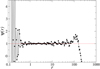 |
Fig. 1. Behavior of the function ψ(r) defined in Eq. (8) at t = 9 Gyr in the case of the initially uniform sphere, where N = 106. At small distances the deviation from ψ = 1 is due to sparse sampling fluctuations while at large distances, (i.e., r > 100 kpc) the deviation is due to the out-of-equilibrium nature of the system. |
Let us now consider the core and the halo of the QSS separately. The core is defined as the region within the length scale r0 found by fitting the density profile with Eq. (9). Figure 2 shows the normalized particle energy distribution of the QSS at t = 9 Gyr (i.e., at a time much longer than τff ≈ 1.5 Gyr). In particular, the three main components of the system after the collapse are highlighted: the first two constitute the actual QSS, namely the core (i.e., r < r0), and the outermost bound particles that forms the halo (r > r0 and e < 0), while the remaining component is comprised of free particles.
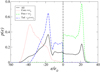 |
Fig. 2. Particle energy distribution of the QSS at t = 9 Gyr in units of e0 (see Eq. (4)). The system after the collapse is made of three components: two form the QSS (tail and core) and the third, where e > 0, is made of “free” particles. The core is comprised of particles with radial distance r < r0; the free particles have positive energy or r > rf, where rf = rf(t) must be estimated from the numerical data. |
A gas under steady-state conditions at a temperature T immersed in a conservative force field is characterized by a distribution function that differs from the Maxwell-Boltzmann (MB) distribution by the exponential factor exp(−Φ(r)/kT), where in this case the temperature can be defined through the particle velocity dispersion. In this situation, the equilibrium distribution function for this case is written as
 (11)
(11)
Consequently, the number density for a system described by this distribution function is given by
 (12)
(12)
The velocity distribution function in the core (see the top and middle panels of Fig. 3) is well approximated by a MB distribution. We carried out the fit by defining the core in two different ways: (i) all particles with r < r0, where r0 was estimated from the best fit of the density profile; and (ii) by considering an energy threshold, that is, e/e0 < −20, where e/e0 = −20 corresponds to the inner peak of p(e) and e0 is defined in Eq. (4). In the latter case the fit is better than in the former. We interpret this as a consequence of the energy threshold selecting the particles in the inner core better than the distance cut because in that case particles that have higher energy, and thus belonging to the halo at a subsequent time, can be confused with the core particles. The temperature T can be thought to be an effective temperature related to an isotropic and scale-independent velocity dispersion, that is, it does not represent a real equilibrium thermodynamical temperature. Figure 3 (bottom panel) shows the almost flat density distribution in the central region where, additionally, the velocity distribution is isotropic.
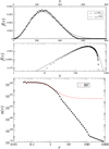 |
Fig. 3. Top panel: velocity distribution function in the core by applying a selection i in energy and the corresponding best fit with a MB distribution with v0 = 250 km s−1 in linear and (middle panel) bi-logarithmic scale. Bottom panel: measured density profile together with the Boltzmann factor (see Eq. (12)). |
Thermal equilibrium is reached in the core driven by two-body collisions. The order of magnitude of the timescale of collisional relaxation is (Binney & Tremaine 2008) given by
 (13)
(13)
where τff is the free-fall time of the system (that has initial density ρ; see Eq. (1)) and τdyn ∼ (Gρ0)−1/2 is the dynamical time of the core with density ρ0 ≫ ρ. In the core (i.e., for r < r0), we find that ρ/ρ0 ∼ 10−5 and N/log(N) ∼ 102 − 103 (log is the decimal logarithm) and thus τ2b ≈ τff: two-body relaxation is efficient enough to establish thermal equilibrium in the core in a timescale of order of τff. We note that an approximate thermal equilibrium is reached in the short timescale corresponding to the global collapse of the system τdyn and that on a much longer timescale, driven by two-body encounters, eventually the QSS that emerges from the violent relaxation process undergoes a gravothermal collapse.
The power-law fit to the density profile is very well defined for r ≥ 4r0. Such a region contains most of the mass of the system and it is surrounded by a lower density region of bound particles, still spherically symmetric distributed, in which the density displays a power-law decay and whose velocity distribution is radially biased. Given these conditions, we aim to find the relation between the exponent α of the power-law fit to the density profile (i.e., ρ(r) ∼ r−α) and the anisotropy parameter β(r) given that the Jeans equation (Eq. (8)) is satisfied. We note that, under the hypotheses mentioned above, the gravitational potential decays, for r > r0, as ϕ(r)∼ − GM0/r – thus corresponding to a force that decays as r−2 (see Fig. 4).
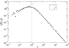 |
Fig. 4. Absolute value of the force as a function of scale in the QSS. |
In this external zone, owing to low density, the self-interaction between particles can be neglected so that the maximum speed of a particle at distance r is the local escape velocity (i.e.,  ; see the top panel of Fig. 5).
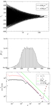 |
Fig. 5. Top panel: radial component of the velocity vr as function of the distance for particles in the tail. Middle panel: example of the velocity distribution f(vr) in a tail shell. Bottom panel: |


By assuming that the probability distribution function (PDF) of vr(r) is uniform in the range ![Mathematical equation: $ [-v_{\rm r}^M(r),v_{\rm r}^M(r)] $](/articles/aa/full_html/2020/11/aa39358-20/aa39358-20-eq22.gif) , a situation that occurs if the system is virialized (see the middle panel of Fig. 5), we find
, a situation that occurs if the system is virialized (see the middle panel of Fig. 5), we find
 (14)
(14)
The bottom panel of Fig. 5 shows that Eq. (14) well approximates the measured behaviors. From Eqs. (8) and (14) we find that for r > r0
 (15)
(15)
If we take β(r) = 1 we find
 (16)
(16)
which well approximates the power-law tail observed in numerical simulations (see Eq. (9)).
In these same approximations we find, for r ≫ r0
 (17)
(17)
However, we urge caution in extrapolating Eq. (17) for any value of β, α. In general the situation is more complicated as neither Eq. (14) nor |ϕ| ∼ 1/r is satisfied when the density decays slower than r−4 and we should consider Eq. (8) instead of Eq. (17) and thus α is expected to have a nontrivial dependence on β and on the whole mass distribution.
In summary, in the case of a violent relaxation of a isolated, cold, spherically symmetric, uniform mass distribution we obtained the limiting behaviors (see Fig. 6)
 (18)
(18)
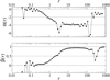 |
Fig. 6. Top panel: radial behavior of the exponent α(r) of the density profile. Bottom panel: radial behavior of the anisotropy parameter β(r). |
3.4. Isolated spherical over-densities with non-Poissonian fluctuations
As discussed Sect. 2 the key parameter of the second family of IC is γ (see Eq. (2)); when γ = 10 the number of centers is only ten times less than the number of particles, and thus fluctuations are slightly greater than in the purely Poissonian case. On the contrary, when γ ≈ 105 the IC consist of subclumps that have collapse timescales shorter than that of the system as a whole. In this situation, subclumps collapse almost independently from each other and then the different substructures merge. A separation of spatial and temporal scales occurs only when the IC is highly inhomogeneous with few centers The intermediate range for γ, 10 < γ < 105, is the most interesting to study.
Figure 7 shows the behavior of the quantity Δ(t), defined by Eq. (3), which measures the amount of energy exchanged among system particles. A clear tread shows that the more uniform the IC the larger is the energy variation. This trend is in line with the Poissonian case, where the larger N is, the smaller the initial fluctuations over the mean and the larger the variation of Δ(t) (Joyce et al. 2009).
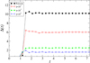 |
Fig. 7. Behavior with time of the quantity Δ(t) (see Eq. (3)) in simulations of isolated spherical over-densities with non-Poissonian fluctuations with different values of γ. The behavior for the case of the initially Poissonian spherical over-densities (black) is shown for comparison. |
Consequently, the asymptotic value of the virial ratio becomes closer to −1 as the energy exchange gets smaller, and thus the amount of particles that have been ejected from the system after the collapse is smaller (see Fig. 8). The reflection of this situation can be clearly seen in the asymptotic shape of the particle energy distribution (see Fig. 9). The more clustered the initial distribution is, the softer the collapse and the less spread p(e) after the collapse.
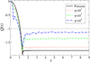 |
Fig. 8. Time evolution of the virial ratio Q in simulations of isolated spherical over-densities with non-Poissonian fluctuations with different γ. The case of the initially Poissonian spherical over-density is also shown for comparison (in black). |
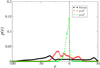 |
Fig. 9. Asymptotic particle energy distribution in the two non-Poissonian simulations. The case of a Poissonian IC is also shown for comparison. |
The density profiles of the QSS in the various simulations are shown by Fig. 10. While there is a clear change of slope in all cases between the inner core and the outer regions, the softer the collapse and the less marked is such a change. That is, while for the uniform case there is a clear change from n(r)∼ const. in the inner core to n(r) ∼ r−4 in the outer regions, when the initial fluctuations are large enough (i.e., γ ≈ 102 − 104), then the density profile in the inner core is closer to n(r) ∼ r−1 and in the outer region to n(r) ∼ r−3.
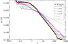 |
Fig. 10. Density profile in the three simulations of isolated spherical over-densities with non-Poissonian fluctuations with different γ. The behavior for the case of the initially Poissonian spherical over-density is also shown for comparison (in black). |
The QSS formed are close to the Jeans equilibrium in all cases. We find that ψ(r)≈1 in an intermediate range of scales between the inner regions, where shot noise fluctuations are predominant, and the outermost regions, where particles have positive energy.
To clarify the statistical and dynamical properties of the QSS we focus on the case in which initial fluctuations are large but the number of subclusters is still large enough so that they have a substantial overlap and thus there is not a separation of length and timescales in the collapsing phases of the whole structure and its substructures. We thus focus on the case γ = 104.
Figure 11 shows the velocity dispersions as a function of distance to the center in the asymptotic QSS. We can identify three different regimes that correspond to the following:
-
(i)
an inner region, in which the dispersion grows slightly inward in an almost isotropic manner (i.e.,
 , corresponding to β(r)≈0,
 -
(ii)
a tail, in which the dispersion (in all components) decreases as a function of the radial distance and
 ,
, -
(iii)
an outermost region, in which
 , that is, where highly energetic particles move on quasi-radial orbits.
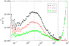 |
Fig. 11. Velocity dispersion (total, transverse, and radial) as a function of distance in the asymptotic QSS for a the case of a very clustered IC, i.e., γ = 104. |
Figure 12 shows the particle energy distribution. Particles in the core are selected as those having r < r0, where in this case r0 approximately coincides with the peak of ⟨v2(r)⟩ (see Fig. 11) and the ejected particles have r > rf, where rf is estimated to be the (time-dependent) scale at which  . The core is populated by the most bound particles, the tail is made by particles with slightly negative energy, while particles in the outermost region have e > 0.
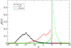 |
Fig. 12. Particle energy distribution in the asymptotic QSS for the case of a very clustered IC, i.e., γ = 104. |
Figure 13 shows the velocity distribution of the particles in the core region. As for the case of the Poissonian IC, a MB distribution represents a good fit, clearly at a much lower temperature (i.e., velocity dispersion) than for the uniform case. We selected the inner regions in two ways: by considering a limit in radial distance (i.e., r < r0) and a limit in energy (e < −10 e0). In the latter case the MB distribution fit better interpolates the data. In the inner core, thermal equilibrium is reached driven by tow-body collisions even in this case.
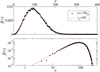 |
Fig. 13. Velocity distribution of the inner regions of the asymptotic QSS for a the case of a very clustered IC, i.e., γ = 104. The selection was performed in energy (i.e., e < 10 e0); the best-fitting Maxwell-Boltzmann distribution is reported. |
Figure 14 shows the density profile in the inner region for γ = 104. Even in this case, the density distribution is well described by Eq. (12). Figure 15 shows the behavior of the anisotropy parameter β(r) (bottom panel) and that of the exponent of the density profile α(r) (top panel) as functions of the distance from the center. We note that, as in the case of the cold uniform spherical over-density, β(r) → 0 in the core and β(r) → 1 in the outermost region; correspondingly the exponent of the density profile α → 0 in the core and α → −4 in the tail. Beyond these two limiting cases it is not possible to obtain an analytical expression of α(β) for the general case. The actual mass distribution is more spread than in the simplest model, where ρ ∼ const. in the inner region and ρ ∼ r−4 in the outer tail. This is quantitatively illustrated by the behavior of the gravitational force in models with different values of γ (see Fig. 16); at short distances from the center the linear growth (implied by a constant matter density) is clear only when γ < 103. For large γ, for instance γ = 104, the force has a short range of radial growth to decay after as r−1 in a intermediate range of distance scales.
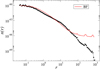 |
Fig. 14. Density profile in the inner core of the asymptotic QSS for the case of a very clustered IC, i.e., γ = 104; the best-fitting with Eq. (12) is also shown. |
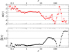 |
Fig. 15. Top panel: behavior of the exponent of the density profile α(r) of a QSS with γ = 104. Bottom panel: behavior of the anisotropy parameter β(r) as a function of the distance from the center. |
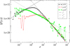 |
Fig. 16. Absolute value of the gravitational force as a function of function of scale in the QSS in simulations with different values of γ. |
3.5. Cosmological halos
As mentioned in Sect. 2 we also considered a set of data extracted 6 from the Abacus simulations (Garrison et al. 2018, 2019) representing the halos typical of cosmological simulations. Their shape is typically ellipsoidal and is characterized by several substructures. Nevertheless, we treat these systems in spherical symmetry, as the ratio between the axes is close to one, and we compute the center as the minimum of the potential energy. A certain degree of arbitrariness in the definition of the outermost cutoff of a halo is present. In this work, we just consider the outputs of the Abacus halo finder keeping in mind that faraway low density particles with high energy may not be included because of a selection effect.
In what follows, we report results for the three more massive halos, H49850, H40661, and H965, which contain, respectively, ∼(8, 4, 3)×105 particles. We checked that when considering smaller halos the results do not qualitatively change but the statistical estimators are noisier.
The density profiles of two halos are shown in the top panel of Fig. 17. The density profile slope changes from α ≈ −1 in the inner region to α = −2 in the outer region of the system. The NFW profile (see Eq. (10)) provides good fits of the behaviors but in the outermost part of the tail, where there is some arbitrariness in the definition of the particle memberships. The radial behavior of the average square velocity resembles that observed in isolated spherical collapse models with non-Poissonian fluctuations (see Fig. 11): indeed, ⟨v2(r)⟩ grows with distance reaching a maximum at ∼r0 and then decays at large distances. The radial and transverse velocity dispersion (not plotted) display a similar behavior. The radial scale r0 roughly separates the two regimes.
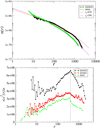 |
Fig. 17. Top panel: density profile in two of most massive halos. The two solid lines represent the best fit for H49850 and H965, respectively, with a NFW profile. Bottom panel: velocity dispersion ⟨v2(r)⟩ for the same halos together with H40661. |
The particle energy distribution in shown in Fig. 18; a small fraction of the particles have positive energy in all the three cases. This fraction clearly depends on the manner in which the external part of the halos has been selected. Differently from Figs. 2 and 9 in this case the energy is normalized to e0 = Wm/M, where W is the gravitational potential energy of the system at redshift z = 0 (i.e., not the initial), M its mass, and m the particle mass: this is clearly much larger (in absolute value) than the initial one. We treat each halo as being isolated; this is clearly an approximation that works better when the halo density contrast is larger. The overall shape of these p(e) is very similar to those obtained in the case of isolated spherical collapse models with non-Poissonian fluctuations and large γ. (see Fig. 9).
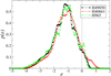 |
Fig. 18. Particle energy distribution in the three largest Abacus halos. In this case the energy is normalized to e0 = Wm/M, where W is the total gravitational potential energy of the system at z = 0 (i.e., not the initial one), M is its mass, and m the particle mass. |
The halos are close to an equilibrium condition as described by the Jeans equation (see Eq. (8)), that is, ψ(r)≈1 (see Fig. 19). At small distances ψ(r) has shot-noise fluctuations while the outermost region of the tail is out of equilibrium as particles have positive energy. In the intermediate region ψ(r) presents larger fluctuations than for the case of the uniform sphere (Fig. 1). This is probably results from the presence of more substructures and the influence of neighboring density perturbations because now these over-densities are not isolated as in the previous cases.
The inner region shows the velocity distribution that is well approximated by a MB distribution (see Fig. 20). Inner region particles were selected by considering a radial distance cut (i.e., r < r0) and, alternatively, an energy cut; in the latter case the MB distribution fits the data better, as for the cases of Figs. 3 and 13. If we use Eq. (12) to compute the density profile of the inner region we obtain a fit that is worse than in the cases discussed previously (see Fig. 21) but that is still reasonably good. On the other hand, the fit is particularly rough at large radial distances. This is probably because the halo is not isolated in these simulations system.
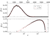 |
Fig. 20. Velocity distribution in the inner core for the most massive Abacus halo (i.e., H49850) together with the best fit with a MB distribution. Inner region particles were selected by considering an energy cut (i.e., e < −2 e0). |
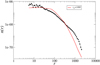 |
Fig. 21. Density profile of the most massive Abacus halo (i.e., H49850). The best-fitting halo with Eq. (12) is also shown. |
Figure 7 shows the behavior of the absolute value of the gravitational force in the three examined massive halos. This value is approximately constant at small radii and then decays as ∼r−1 at large distances, which is a behavior consistent with the density profile shown in Fig. 17. The large fluctuations in the force profile, especially for the case of the halo H49850, are due to substructures. Finally, the anisotropy parameter (bottom panel of Fig. 22) is β ≈ 0 in the inner zone (where n(r) ∼ r−1), while β ≈ 0.5 in the outer regions of the system (where n(r) ∼ r−2).
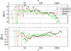 |
Fig. 22. Top panel: derivative of the density profile for the three largest Abacus halos. Bottom panel: anisotropy parameter. |
3.6. Discussion
In high-resolution simulations of CDM halos (Taylor & Navarro 2001) the coarse-grained phase-space density decays as
 (19)
(19)
where μ ≈ 1.875. We compare the results of our experiment with the above behavior, starting from the violent collapse case of a uniform sphere. In this case, combining Eqs. (9) and (14) we find μ = 5/2 in the tail, while in the core μ ≃ 0 (see top panel of Fig. 23). The QSS established after the collapse of spherical distributions with non-Poissonian fluctuations show a behavior that depends on the parameter γ: when γ is small, and thus the initial fluctuations are close to Poissonian, then the slope μ is similar to that of the Poissonian case. When instead the distribution is initially clustered (i.e., γ = 103 − 104), then the slope is μ ≈ 1.875 (see the middle panel of Fig. 23).
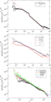 |
Fig. 23. Coarse-grained phase-space density in the uniform case (top panel), nonuniform case (middle panel), and cosmological halos (bottom panel). |
The different behavior observed for the isolated and clustered simulations as a function of γ is again good evidence that, by changing such a parameter, the mean-field and collisionless dynamics that drive system to reach a QSS passes from being close to a top-down monolithic collapse to a bottom-up hierarchical aggregation process. Finally, in the cosmological halos of the Abacus simulations of the previous subsection we find μ ≈ 1.875, thus very similar to the isolated case with γ = 103 − 104 (see the bottom panel of Fig. 23).
For the case of cosmological halos, there have been attempts to determine the slope of the density profile α for spherically symmetric and isotropic systems that are in Jeans equilibrium and that exhibit power-law, coarse-grained, phase-space density (Taylor & Navarro 2001). It was formally shown that the allowed density slopes α lie in the range [1, 3] (Hansen 2004). It was then noticed that in halos extracted from cosmological simulations there is a linear relationship between the density slope and the anisotropy parameter (Hansen & Moore 2006; Hansen & Stadel 2006; Hansen et al. 2006); this relationship, however, has a large scattering, where for α → 3 for β → 0.5 and α → 1 for β → 0. These trends are similar to what we obtain in examining the Abacus halos, but not for case in which the more violent relaxation occurring when a monolithic collapse takes place as in this latter case α → 0 for β → 0. This situation thus shows that the relation between α and β is determined by the dynamical mechanism at work rather being universal as argued by Hansen & Moore (2006).
From an analytical point of view, by using the hypotheses that both the coarse-grained phase-space density and the density profile being a power law in distance, allowing for the possibility that the velocity distribution is not isotropic and the empirical linear relation between α and β, it is possible to solve the Jeans equations analytically and extract the relevant statistical information of the system (Dehnen & McLaughlin 2005). However, a purely power-law, coarse-grained, phase-space density approximates well the observed behavior only for the case of a bottom-up dynamics but not for the top-down case.
4. Conclusions
Two competing processes work to determine the dynamical evolution of finite initially spherical and cold self-gravitating systems. On one hand they undergo a global (top-down) collapse driven by their own rapidly varying gravitational field, and, on the other hand, internal density fluctuations lead to formation of local substructures of growing size through a (bottom-up) aggregation process. Therefore, in general, there is a sort of competition between a top-down and a bottom-up mean-field collisionless dynamics. Anyway, in both cases collisional effects are negligible because of their much longer timescale with respect to that giving rise to QSS.
The properties of the QSS formed depend on the evolutionary paths they have followed, and thus on which of the above-mentioned two mechanisms prevails during the relaxation from the out-of-equilibrium IC to the quasi-stationary configuration. In particular, the dynamics is different depending on the type of correlation properties between initial density perturbations. When the amplitude of initial fluctuations is small, a global collapse takes place and the system relaxes into a QSS in a very short time: the signature of this process is a wide energy exchange between particles. On the other hand, in case of large initial fluctuations, the bottom-up aggregation process becomes predominant over the global collapse and, so, clustering at small scales builds up larger and larger substructures halting the global collapse. That is, the fragmentation into large and growing substructures inhibits the occurrence of a large variation of the overall system size and, consequently, the particle energy distribution only moderately changes.
We considered a family of simple IC representing isolated, spherical, and cold distributions of particles with different spectra of initial density fluctuations. By varying the initial amplitude of initial density perturbations, we find that it is possible to select the mechanism through which the out-of-equilibrium IC are driven to form a QSS.
As we said above, for the case of a top-down (monolithic) collapse, which occurs whenever the amplitude of initial density fluctuations are small, the particle energy distribution changes significantly in a rapid interval of time centered around the time of maximum system contraction (essentially the free-fall time): such variation is given by the interplay of the finite size of the system with the growth of density perturbations during the collapse. In this situation, the QSS are characterized by a compact core, which contains a significant fraction of the system mass and shows an almost isotropic velocity distribution. The core is surrounded by a low-density region in which orbits are very elongated, that is, where the velocity anisotropy parameter β tends to 1. Based on an assumption of the validity of the Jeans equation, we were able to show that the inner region of a system emerging by a violent top-down collapse is characterized by an almost flat density profile. However, the outer power-law decay of density is ρ(r) ∼ r−4, a behavior that is observed in the numerical experiments of initially cold and uniform systems.
On the other hand, when initial perturbations are of large enough amplitude then a QSS is reached through a bottom-up, hierarchical, aggregation process in which small substructures merge to form larger and larger substructures. This process is accelerated when initial density correlations are long range. That is, at given initial fluctuations amplitude, the smaller the power-law index, n ∈ ( − 3, 0], of the density fluctuation power spectrum, P(k) ∼ kn, the faster the evolution of the bottom-up mechanism of structure formation. In this latter situation, the variation of the particle energy distribution is smaller than in the former and, for this reason, the orbits in the outermost regions of the system are less radially elongated. The exponent of the density profile is 0 < α ≤ 4 and the anisotropy parameter is 0 ≤ β < 1. When initial density perturbations are large enough the core-halo structure is not formed. In this case the profile is better fitted by a NFW behavior.
We also demonstrated that the halos formed in cosmological N-body simulations in the standard CDM scenario, although they are not isolated but rather embedded in the tidal field of neighboring structures, show properties similar to QSS obtained in the simple isolated and spherical cases considered in this work, in the case of large enough initial fluctuation amplitudes. In CDM-like cosmologies, density fluctuations are long-range correlated (i.e., P(k) ∼ k−2) and, as said above, this situation implies the development of a bottom-up aggregation process rather than a top-down scenario through the collapse of large over-densities. We can thus conclude that isolated, spherical, and dynamically cold systems with different choices of initial density perturbations amplitude represent a useful tool to study the formation of QSS through a mean-field collisionless dynamics, both when the clustering proceeds in a bottom-up and in top-down way. The fact that systems emerging from cosmological environment have similar properties to those emerging from isolated IC a imply that, when fluctuations are highly nonlinear, the evolution of a cosmological halo is well approximated by neglecting tidal interactions with neighboring structures.
To conclude, we now consider a long-standing observational puzzle that can be related to these results. This is the core-cusp problem, that is, the well-known difference between the observed inner density profiles of dark matter in low-mass galaxies and the density profiles obtained in cosmological N-body simulations. Observations seem to indicate an approximately constant dark matter density in the inner parts of galaxies (the core), while CDM halos profiles show instead a ∼r−1 power-law cusp at short distances (Navarro et al. 1997). This fact, known as the “core/cusp controversy”, stands as one of the unsolved problems in small-scale cosmology (see for a recent review De Blok 2010 and references therein). Our results suggest that a possible solution to this puzzle could be found in the violent origin of the galaxies through something more similar to a monolithic collapse than a bottom-up aggregation process. Benhaiem et al. (2017, 2019), Sylos Labini et al. (2020) provide further discussions of this specific topic. Concerning the latter point, we note that the case for galaxy formation through a monolithic collapse has also been very recently advocated by Peebles (2020).
The virial ratio q is defined in this work as  , where K and W are the total kinetic and potential energy, respectively.
Data are available from https://lgarrison.github.io/AbacusCosmos/
This is a hybrid algorithm described in https://abacussummit.readthedocs.io/en/latest/compaso.html
The convention that a = 1 at z = 0 was used, so the proper and comoving softening lengths are both equal to 7 kpc h−1 at z = 0.
Unless specified all distances are expressed in kpc and all times in Gyr. The velocities are measured in km s−1.
Acknowledgments
We are grateful to Lehman Garrison for his valuable assistance in explaining us the Abacus database and for providing us an ad-hoc simulation with high resolution halos catalogs and data. The Abacus data are available at https://lgarrison.github.io/AbacusCosmos/. We are grateful to Volker Springel for his help in the use of Gadget-2.
References
- Aarseth, S., Lin, D., & Papaloizou, J. 1988, ApJ, 324, 288 [NASA ADS] [CrossRef] [Google Scholar]
- Aguilar, L., & Merritt, D. 1990, ApJ, 354, 73 [NASA ADS] [CrossRef] [Google Scholar]
- Arca-Sedda, M., & Capuzzo-Dolcetta, R. 2014, ApJ, 785, 51 [NASA ADS] [CrossRef] [Google Scholar]
- Barnes, E. I., Lanzel, P. A., & Williams, L. L. R. 2009, ApJ, 704, 372 [NASA ADS] [CrossRef] [Google Scholar]
- Baushev, A., & Barkov, M. 2018, JCAP, 2018, 034 [CrossRef] [Google Scholar]
- Benetti, F. P. C., Ribeiro-Teixeira, A. C., Pakter, R., & Levin, Y. 2014, Phys. Rev. Lett., 113, 100602 [CrossRef] [Google Scholar]
- Benhaiem, D., & Sylos Labini, F. 2015, MNRAS, 448, 2634 [NASA ADS] [CrossRef] [Google Scholar]
- Benhaiem, D., & Sylos Labini, F. 2017, A&A, 598, A95 [CrossRef] [EDP Sciences] [Google Scholar]
- Benhaiem, D., Joyce, M., Sylos Labini, F., & Worrakitpoonpon, T. 2016, A&A, 585, A139 [NASA ADS] [CrossRef] [EDP Sciences] [Google Scholar]
- Benhaiem, D., Joyce, M., & Sylos Labini, F. 2017, ApJ, 851, 19 [NASA ADS] [CrossRef] [Google Scholar]
- Benhaiem, D., Sylos Labini, F., & Joyce, M. 2019, Phys. Rev. E, 99, 022125 [NASA ADS] [CrossRef] [Google Scholar]
- Binney, J., & Knebe, A. 2001, MNRAS, 325, 845 [NASA ADS] [CrossRef] [Google Scholar]
- Binney, J., & Tremaine, S. 2008, Galactic Dynamics: Second Edition (Princeton: Princeton University Press) [Google Scholar]
- Blumenthal, G. R., Pagels, H., & Primack, J. R. 1982, Nature, 299, 37 [NASA ADS] [CrossRef] [Google Scholar]
- Blumenthal, G. R., Faber, S. M., Primack, J. R., & Rees, M. J. 1984, Nature, 311, 517 [NASA ADS] [CrossRef] [Google Scholar]
- Boily, C. M., & Athanassoula, E. 2006, MNRAS, 369, 608 [NASA ADS] [CrossRef] [Google Scholar]
- Boily, C., Athanassoula, E., & Kroupa, P. 2002, MNRAS, 332, 971 [NASA ADS] [CrossRef] [Google Scholar]
- Bond, J. R., Szalay, A. S., & Turner, M. S. 1982, Phys. Rev. Lett., 48, 1636 [NASA ADS] [CrossRef] [Google Scholar]
- Campa, A., Dauxois, T., Fanelli, D., & Ruffo, S. 2014, Physics of Long-Range Interacting Systems (Oxford: Oxford University Press) [CrossRef] [Google Scholar]
- Capuzzo-Dolcetta, R. A. 2019, Classical Newtonian Gravity (Springer International Publishing) [CrossRef] [Google Scholar]
- Dauxois, T., Ruffo, S., Arimondo, E., & Wilkens, M. 2002, Dynamics and Thermodynamics of Systems with Long-Range Interactions: An Introduction (Berlin, Heidelberg: Springer), 1 [Google Scholar]
- De Blok, W. J. G. 2010, Adv. Astron., 2010, 789293 [NASA ADS] [CrossRef] [Google Scholar]
- Dehnen, W. 1993, MNRAS, 265, 250 [NASA ADS] [CrossRef] [Google Scholar]
- Dehnen, W., & McLaughlin, D. E. 2005, MNRAS, 363, 1057 [NASA ADS] [CrossRef] [MathSciNet] [Google Scholar]
- Diemand, J., Moore, B., Stadel, J., & Kazantzidis, S. 2004, MNRAS, 348, 977 [CrossRef] [Google Scholar]
- Garrison, L. H., Eisenstein, D. J., Ferrer, D., et al. 2018, ApJS, 236, 43 [CrossRef] [Google Scholar]
- Garrison, L. H., Eisenstein, D. J., & Pinto, P. A. 2019, MNRAS, 485, 3370 [CrossRef] [Google Scholar]
- Hansen, S. H. 2004, MNRAS, 352, L41 [NASA ADS] [CrossRef] [Google Scholar]
- Hansen, S. H., & Moore, B. 2006, New Astron., 11, 333 [NASA ADS] [CrossRef] [Google Scholar]
- Hansen, S. H., & Stadel, J. 2006, JCAP, 2006, 014 [Google Scholar]
- Hansen, S., Moore, B., & Stadel, J. 2006, EAS Publ. Ser., 20, 33 [CrossRef] [Google Scholar]
- Henon, M. 1964, Ann. Astrophys., 27, 1 [Google Scholar]
- Jeans, J. H. 1915, MNRAS, 76, 70 [NASA ADS] [CrossRef] [Google Scholar]
- Joyce, M., & Sylos Labini, F. 2013, MNRAS, 429, 1088 [NASA ADS] [CrossRef] [Google Scholar]
- Joyce, M., Marcos, B., & Sylos Labini, F. 2009, MNRAS, 397, 775 [NASA ADS] [CrossRef] [Google Scholar]
- Levin, Y., Pakter, R., & Rizzato, F. 2008, Phys. Rev. E, 78, 021130 [NASA ADS] [CrossRef] [Google Scholar]
- Levin, Y., Pakter, R., Rizzato, F. B., Teles, T. N., & Benetti, F. P. 2014, Phys. Rep., 535, 1 [CrossRef] [Google Scholar]
- Lynden-Bell, D. 1967, MNRAS, 136, 101 [NASA ADS] [CrossRef] [Google Scholar]
- Merritt, D., & Aguilar, L. A. 1985, MNRAS, 217, 787 [NASA ADS] [CrossRef] [Google Scholar]
- Navarro, J. F., Frenk, C. S., & White, S. D. M. 1997, ApJ, 490, 493 [NASA ADS] [CrossRef] [Google Scholar]
- Navarro, J. F., Hayashi, E., Power, C., et al. 2004, MNRAS, 349, 1039 [NASA ADS] [CrossRef] [Google Scholar]
- Padmanabhan, T. 1990, Phys. Rep., 188, 285 [NASA ADS] [CrossRef] [MathSciNet] [Google Scholar]
- Peebles, P. J. E. 1980, The Large-Scale Structure of the Universe (Princeton: Princeton University Press) [Google Scholar]
- Peebles, P. J. E. 2020, MNRAS, 498, 4386 [CrossRef] [Google Scholar]
- Roy, F., & Perez, J. 2004, MNRAS, 348, 62 [NASA ADS] [CrossRef] [Google Scholar]
- Sahni, V., & Coles, P. 1995, Phys. Rep., 262, 1 [NASA ADS] [CrossRef] [Google Scholar]
- Spera, M., & Capuzzo-Dolcetta, R. 2017, Astrophys. Space Sci., 362, 233 [CrossRef] [Google Scholar]
- Springel, V. 2005, MNRAS, 364, 1105 [NASA ADS] [CrossRef] [Google Scholar]
- Sylos Labini, F. 2012, MNRAS, 423, 1610 [NASA ADS] [CrossRef] [Google Scholar]
- Sylos Labini, F. 2013a, MNRAS, 429, 679 [NASA ADS] [CrossRef] [Google Scholar]
- Sylos Labini, F. 2013b, A&A, 552, A36 [NASA ADS] [CrossRef] [EDP Sciences] [Google Scholar]
- Sylos Labini, F., Benhaiem, D., & Joyce, M. 2015, MNRAS, 449, 4458 [NASA ADS] [CrossRef] [Google Scholar]
- Sylos Labini, F., Pinto, L. D., & Capuzzo-Dolcetta, R. 2020, Phys. Rev. E, 102, 042108 [CrossRef] [Google Scholar]
- Taylor, J. E., & Navarro, J. F. 2001, ApJ, 563, 483 [NASA ADS] [CrossRef] [Google Scholar]
- Theis, C., & Spurzem, R. 1999, A&A, 341, 361 [NASA ADS] [Google Scholar]
- van Albada, T. 1982, MNRAS, 201, 939 [NASA ADS] [CrossRef] [Google Scholar]
- Worrakitpoonpon, T. 2015, MNRAS, 466, 1335 [NASA ADS] [CrossRef] [Google Scholar]
All Figures
|
Fig. 1. Behavior of the function ψ(r) defined in Eq. (8) at t = 9 Gyr in the case of the initially uniform sphere, where N = 106. At small distances the deviation from ψ = 1 is due to sparse sampling fluctuations while at large distances, (i.e., r > 100 kpc) the deviation is due to the out-of-equilibrium nature of the system. |
| In the text | |
|
Fig. 2. Particle energy distribution of the QSS at t = 9 Gyr in units of e0 (see Eq. (4)). The system after the collapse is made of three components: two form the QSS (tail and core) and the third, where e > 0, is made of “free” particles. The core is comprised of particles with radial distance r < r0; the free particles have positive energy or r > rf, where rf = rf(t) must be estimated from the numerical data. |
| In the text | |
|
Fig. 3. Top panel: velocity distribution function in the core by applying a selection i in energy and the corresponding best fit with a MB distribution with v0 = 250 km s−1 in linear and (middle panel) bi-logarithmic scale. Bottom panel: measured density profile together with the Boltzmann factor (see Eq. (12)). |
| In the text | |
|
Fig. 4. Absolute value of the force as a function of scale in the QSS. |
| In the text | |
|
Fig. 5. Top panel: radial component of the velocity vr as function of the distance for particles in the tail. Middle panel: example of the velocity distribution f(vr) in a tail shell. Bottom panel: |
| In the text | |
|
Fig. 6. Top panel: radial behavior of the exponent α(r) of the density profile. Bottom panel: radial behavior of the anisotropy parameter β(r). |
| In the text | |
|
Fig. 7. Behavior with time of the quantity Δ(t) (see Eq. (3)) in simulations of isolated spherical over-densities with non-Poissonian fluctuations with different values of γ. The behavior for the case of the initially Poissonian spherical over-densities (black) is shown for comparison. |
| In the text | |
|
Fig. 8. Time evolution of the virial ratio Q in simulations of isolated spherical over-densities with non-Poissonian fluctuations with different γ. The case of the initially Poissonian spherical over-density is also shown for comparison (in black). |
| In the text | |
|
Fig. 9. Asymptotic particle energy distribution in the two non-Poissonian simulations. The case of a Poissonian IC is also shown for comparison. |
| In the text | |
|
Fig. 10. Density profile in the three simulations of isolated spherical over-densities with non-Poissonian fluctuations with different γ. The behavior for the case of the initially Poissonian spherical over-density is also shown for comparison (in black). |
| In the text | |
|
Fig. 11. Velocity dispersion (total, transverse, and radial) as a function of distance in the asymptotic QSS for a the case of a very clustered IC, i.e., γ = 104. |
| In the text | |
|
Fig. 12. Particle energy distribution in the asymptotic QSS for the case of a very clustered IC, i.e., γ = 104. |
| In the text | |
|
Fig. 13. Velocity distribution of the inner regions of the asymptotic QSS for a the case of a very clustered IC, i.e., γ = 104. The selection was performed in energy (i.e., e < 10 e0); the best-fitting Maxwell-Boltzmann distribution is reported. |
| In the text | |
|
Fig. 14. Density profile in the inner core of the asymptotic QSS for the case of a very clustered IC, i.e., γ = 104; the best-fitting with Eq. (12) is also shown. |
| In the text | |
|
Fig. 15. Top panel: behavior of the exponent of the density profile α(r) of a QSS with γ = 104. Bottom panel: behavior of the anisotropy parameter β(r) as a function of the distance from the center. |
| In the text | |
|
Fig. 16. Absolute value of the gravitational force as a function of function of scale in the QSS in simulations with different values of γ. |
| In the text | |
|
Fig. 17. Top panel: density profile in two of most massive halos. The two solid lines represent the best fit for H49850 and H965, respectively, with a NFW profile. Bottom panel: velocity dispersion ⟨v2(r)⟩ for the same halos together with H40661. |
| In the text | |
|
Fig. 18. Particle energy distribution in the three largest Abacus halos. In this case the energy is normalized to e0 = Wm/M, where W is the total gravitational potential energy of the system at z = 0 (i.e., not the initial one), M is its mass, and m the particle mass. |
| In the text | |
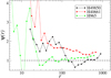 |
Fig. 19. Behavior of the parameter ψ(r) (see Eq. (8)) for the three largest Abacus halos. |
| In the text | |
|
Fig. 20. Velocity distribution in the inner core for the most massive Abacus halo (i.e., H49850) together with the best fit with a MB distribution. Inner region particles were selected by considering an energy cut (i.e., e < −2 e0). |
| In the text | |
|
Fig. 21. Density profile of the most massive Abacus halo (i.e., H49850). The best-fitting halo with Eq. (12) is also shown. |
| In the text | |
|
Fig. 22. Top panel: derivative of the density profile for the three largest Abacus halos. Bottom panel: anisotropy parameter. |
| In the text | |
|
Fig. 23. Coarse-grained phase-space density in the uniform case (top panel), nonuniform case (middle panel), and cosmological halos (bottom panel). |
| In the text | |
Current usage metrics show cumulative count of Article Views (full-text article views including HTML views, PDF and ePub downloads, according to the available data) and Abstracts Views on Vision4Press platform.
Data correspond to usage on the plateform after 2015. The current usage metrics is available 48-96 hours after online publication and is updated daily on week days.
Initial download of the metrics may take a while.