| Issue |
A&A
Volume 643, November 2020
|
|
|---|---|---|
| Article Number | A57 | |
| Number of page(s) | 7 | |
| Section | Atomic, molecular, and nuclear data | |
| DOI | https://doi.org/10.1051/0004-6361/202038659 | |
| Published online | 03 November 2020 | |
Plasma environment effects on K lines of astrophysical interest
IV. IPs, K thresholds, radiative rates, and Auger widths in Fe II–Fe VIII⋆
1
Physique Atomique et Astrophysique, Université de Mons – UMONS, 7000 Mons, Belgium
e-mail: patrick.palmeri@umons.ac.be
2
Department of Physics, Western Michigan University, Kalamazoo, MI 49008, USA
3
Helmholtz Institut Jena, 07743 Jena, Germany
4
Theoretisch Physikalisches Institut, Friedrich Schiller Universität Jena, 07743 Jena, Germany
5
Cahill Center for Astronomy and Astrophysics, California Institute of Technology, Pasadena, CA 91125, USA
6
Dr. Karl Remeis-Observatory and Erlangen Centre for Astroparticle Physics, Sternwartstr. 7, 96049 Bamberg, Germany
7
NASA Goddard Space Flight Center, Code 662, Greenbelt, MD 20771, USA
8
IPNAS, Université de Liège, Sart Tilman, 4000 Liège, Belgium
Received:
15
June
2020
Accepted:
15
September
2020
Aims. Within the framework of compact-object accretion disks, we calculate plasma environment effects on the atomic structure and decay parameters used in the modeling of K lines in lowly charged iron ions, namely Fe II–Fe VIII.
Methods. For this study, we used the fully relativistic multiconfiguration Dirac–Fock method approximating the plasma electron–nucleus and electron-electron screenings with a time-averaged Debye-Hückel potential.
Results. We report modified ionization potentials, K-threshold energies, wavelengths, radiative emission rates, and Auger widths for plasmas characterized by electron temperatures and densities in the ranges 105 − 107 K and 1018 − 1022 cm−3. In addition, we propose two universal fitting formulae to predict the IP and K-threshold lowerings in any elemental ion.
Conclusions. We conclude that the high-resolution X-ray spectrometers onboard the future XRISM and ATHENA space missions will be able to detect the lowering of the K edges of these Fe ions due to the extreme plasma conditions occurring in the accretion disks around compact objects.
Key words: black hole physics / plasmas / atomic data / X-rays: general
Full Table 4 is only available at the CDS via anonymous ftp to cdsarc.u-strasbg.fr (130.79.128.5) or via http://cdsarc.u-strasbg.fr/viz-bin/cat/J/A+A/643/A57
© ESO 2020
1. Introduction
This is the fourth paper in a series dedicated to plasma density effects on relevant atomic parameters that are used to model K lines in ions of astrophysical interest, namely, the ionization potentials, K thresholds, transition wavelengths, radiative emission rates, and Auger widths. The data have been computed with the relativistic multiconfiguration Dirac–Fock (MCDF) method (Grant et al. 1980; McKenzie et al. 1980; Grant 1988), as implemented in the GRASP92 (Parpia et al. 1996) and RATIP (Fritzsche 2012) atomic structure packages. The plasma electron–nucleus and electron–electron shieldings are approximated with a time-averaged Debye-Hückel (DH) potential. The datasets comprise the following ionic species: O I–O VII, by Deprince et al. (2019a, hereafter Paper I); Fe XVII–Fe XXV, by Deprince et al. (2019b, hereafter Paper II); Fe IX–Fe XVI, by Deprince et al. (2020, hereafter Paper III).
Here, we report the corresponding density modified radiative data for the fourth-row Fe ions, Fe II–Fe VIII, by applying the same method.
The inner regions of the accretion disks of compact objects display plasmas with densities in the range between 1015 − 1022 cm−3, where absorption and emission of high-energy photons occur. The emerging X-rays can be observed with current space telescopes such as NuSTAR, Chandra, and XMM-Newton. Spectral modeling can provide measurements of the composition, temperature, and degree of ionization of the plasma (Ross & Fabian 2005; García & Kallman 2010). For example, the distortion of the Fe K lines by the strong relativistic effects constrains the angular momentum of the central black hole (Reynolds 2013; García et al. 2014). However, the vast majority of the atomic parameters used to synthesize the X-ray spectra involving K-shell processes do not take density effects into account, thus compromising their usefulness in abundance determinations beyond densities of 1018 cm−3 (Smith & Brickhouse 2014). The aim of the present work is to contribute to remedy this deficiency.
2. Theoretical approach
We outline, in what follows, the main modifications introduced in the MCDF formalism to handle the density effects in a weakly coupled plasma. More details can be found in Papers I–II.
The Debye-Hückel screened Dirac–Coulomb Hamiltonian (Saha & Fritzsche 2006) is given by
where rij = |ri − rj| and the plasma screening parameter μ is the inverse of the Debye shielding length λD. The screening parameter can be expressed in atomic units (au) in terms of the plasma electron density ne and temperature Te as:
For the typical plasma conditions in black-hole accretion disks, Te ∼ 105 − 107 K and ne ∼ 1018 − 1022 cm−3 (Schnittman et al. 2013), the screening parameter μ spans the range 0.0–0.24 au. The Debye-Hückel screening theory is only valid for a weakly coupled plasma where its thermal energy dominates its electrostatic energy. This can be parameterized by the plasma coupling parameter Γ defined by
where Z* is the average plasma ionic charge or ionization,
with ni, X as the number density of an ion, i, of an element, X, bearing a positive charge, zi, X, and d measuring the interparticle distance,
The plasma neutrality implies
and, therefore, Eqs. (4) and (5) can be rewritten as:
If we take a fully-ionized hydrogen plasma with Z* = 1, the plasma coupling parameter falls in the interval 0.0003 ≤ Γ ≤ 0.3 for the typical conditions in black-hole accretion disks. This is well below 1, which fulfills the criteria of a weakly coupled plasma. Even though we could consider a more realistic cosmic plasma with a mixture of 90% hydrogen with 10% helium, both fully ionized, that is, Z* = 0.9 + 2 × 0.1 = 1.1 (with the necessity of multiplying the limits of the above interval by Z*2/3 ∼ 1.07), the plasma coupling parameter values would still agree with a weakly coupled plasma. However, it might be not so in the unlikely scenario of a black-hole accretion disk made of a fully-ionized uranium plasma, with Z* = 92. In this case, we would have Γ ∼ 6 in the coolest and densest regions, where Te ∼ 105 K and ne ∼ 1022 cm−3.
As we already reported in Paper I, this method has been successfully tested, reproducing the experimental Stark shifts of valence transitions of O II (with μ = 0.0017 au) (Djenize et al. 1998) and of Na I (with μ = 0.0023 au) (Sreckovic et al. 1996) but also the Ti Kα line pressure shift (with μ = 0.27 au) measured in the laboratory by Khattak et al. (2012). However, here, we underline the fact that in all these test cases, the differences between the MCDHF/RATIP wavelengths and transition energies, and the corresponding experimental values, were of the order of ∼0.2%, all the while obtaining calculated plasma shifts that are in good agreement with the measurements. For instance, in the case of the  Ti XXI transition, Khattak et al. (2012) measured a line shift of 3.4 eV from the un-shifted position at 4749.73 eV measured by Beiersdorfer et al. (1989). Our corresponding MCDHF/RATIP values are 3.3 eV and 4758.6 eV, respectively.
In this work, the MCDF expansions for Fe II–Fe VIII are built up using the active space (AS) method, whereby we consider all the single and double electron excitations from reference configurations (Table 1) to configurations including n = 3 and 4s orbitals. The final number of CSFs included in the MCDF model for each ion is also listed therein.
Reference configurations used to build up the MCDF active space (AS) listing the total number of configuration state functions (CSFs), NCSF, generated for the MCDF expansions in Fe II–Fe VIII.
Following the computations reported in Papers I–III, the extended average level (EAL) option is used to optimize a weighted trace of the Hamiltonian, using level weights proportional to (2J + 1) that includes QED effects. The combination of the GRASP2K and RATIP programs is used to model the atomic structure to obtain wavelengths, transition probabilities, and Auger widths associated with K-vacancy states. Plasma environment effects are taken into account for a Debye screening parameter in the range 0 ≤ μ ≤ 0.25 au.
3. Results and discussion
3.1. Ionization potentials and K thresholds
The computed ionization potentials (IPs) and K thresholds (EK) are reported in Tables 2 and 3, respectively, for plasma screening parameters, μ = 0.0 au (isolated atomic system), μ = 0.1 au, and μ = 0.25 au. For the isolated ion case, the comparison in Table 2 of the computed IPs with the spectroscopic values in the atomic database of the National Institute of Standards and Technology (Kramida et al. 2019, NIST) shows good overall agreement (within 1%) except for Fe II and Fe III where it deteriorates to 16% and 7%, respectively. This outcome reflects numerical difficulties in modeling the complex atomic structure of iron ions in the neutral end of the isonuclear sequence, especially when trying to obtain accurate representations for both the IP and the highly excited K-vacancy states.
Computed ionization potentials for Fe II–Fe VIII as a function of the plasma screening parameter μ (au).
Computed K-thresholds for Fe II–Fe VIII as a function of the plasma screening parameter μ (au).
The IP and K-threshold lowerings due to plasma effects can also be appreciated in Tables 2 and 3 for μ = 0.1 au and μ = 0.25 au. The IPs of Fe II–Fe VIII are reduced by 4.7–21.3 eV for μ = 0.1 au and by 11.1–51.2 eV for μ = 0.25 au, while the corresponding K thresholds are reduced by 4.9–22.4 eV and by 15.9–58.5 eV, respectively. The IP and K-threshold shifts are found to be close in magnitude (a difference of only a few eV is observed for μ = 0.25 au) as was previously reported for Fe IX–Fe XXV in Papers II and III. The IP percentage downshifts are 14–25% for μ = 0.1 au and 36–59% for μ = 0.25 au; meaning that the IP relative lowering is large for the lowly ionized Fe species. In contrast, the K-threshold percentage downshifts are less than 1% due to their large level energies, but their absolute shifts can be as high as 60 eV.
As shown in Figs. 1 and 2, the IP lowering varies linearly with both the plasma screening parameter μ and effective charge (Zeff = Z − N + 1), except for a small discontinuity between Zeff = 3 and Zeff = 4 caused by the opening of the N shell (n = 4) in Fe III, which becomes more conspicuous for μ = 0.25 au. This effect was already observed in the closing of the L and K shells in Fe XVII and Fe XXV, respectively, as reported in Paper III.
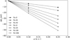 |
Fig. 1. Ionization potential shifts in Fe IX–Fe XXV as a function of the plasma screening parameter μ. Squares: Fe II. Circles: Fe III. Upright triangles: Fe IV. Downright triangles: Fe V. Rightward triangles: Fe VI. Leftward triangles: Fe VII. Stars: Fe VIII. |
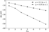 |
Fig. 2. Ionization potential shifts in Fe IX–Fe XXV as a function of the effective charge Zeff = Z − N + 1. Squares: μ = 0.1 au. Circles: μ = 0.25 au. |
As shown in Fig. 3, the ionization potential increases linearly with Zeff, except for a jump of a factor of 1.5 between Zeff = 8 and Zeff = 9 and a gradient change between Zeff = 3 and Zeff = 4. The NIST values (Kramida et al. 2019) are also plotted (the error bars are too small to be seen) for a comparison with our isolated-atom model (μ = 0 au) showing that same jump. The latter is attributed to the closing of the 3p subshell, as it is similar to those displayed by Fe XVII and Fe XXV by the respective closing of the L and K shells (see Paper III) and the gradient change is due to the opening of the N shell. On the other hand, as previously reported in Paper III, the K-threshold trend is somewhat different: it also increases linearly with Zeff but the slope becomes steeper at Fe IV and Fe IX (see Fig. 4). This is also due to shell opening and closing effects but it is less appreciable than for the IP since the K-shell electron is located closer to the nucleus as mentioned in Paper III. In any case, for both the IP and K threshold, the jump (79.8 eV, 77.1 eV, and 73.5 eV for μ = 0 au, μ = 0.1, au and μ = 0.25 au, respectively) as well as the slope change are slightly attenuated as the plasma screening parameter increases.
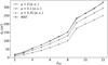 |
Fig. 3. Ionization potential of Fe II–Fe XII as a function of the effective charge Zeff = Z − N + 1. Circles: μ = 0 au (isolated atom). Squares: μ = 0.1 au. Triangles: μ = 0.25 au. Stars: NIST (Kramida et al. 2019). |
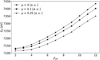 |
Fig. 4. K thresholds of Fe II–Fe XII as a function of the effective charge Zeff = Z − N + 1. Circles: μ = 0 au (isolated atom). Squares: μ = 0.1 au. Triangles: μ = 0.25 au. |
3.2. Radiative transitions
Wavelengths and radiative transition rates for the strongest K lines (Aki ≥ 1013 s−1) in Fe II–Fe VIII are reported in Table 4 for μ = 0 au, μ = 0.1 au and μ = 0.25 au. Our K-line wavelengths are in good agreement with the HFR values computed by Palmeri et al. (2003) as they differ by less than 0.2%, but the radiative rates only agree to within 15–20%. The latter is the result of the strong mixing between states containing both 3d and 4s orbitals in Fe II and Fe III, which causes larger uncertainties in the transition probabilities computed with the HFR and MCDF methods.
Wavelengths and transition probabilities for the K lines of Fe II–Fe VIII (2 ≤ Zeff ≤ 8) computed with plasma screening parameters μ = 0.0, 0.1, and 0.25 au.
In Table 5, our MCDF/RATIP centroid wavelengths of the Kα1, 2 and Kβ unresolved transition arrays are compared with the EBIT measurements of Decaux et al. (1995) in Fe X and the solid-state measurements of Hölzer et al. (1997) (Fe II). In order for us to determine the centroid wavelengths, the MCDF/RATIP wavelengths were weighted with their corresponding transition probabilities, with the data for Fe X taken from Paper III. We can see that the differences between the isolated-atom values (μ = 0 au) and the measurements are up to ∼4 mÅ or ∼0.2%, that is, in line with the expected accuracy determined in our test cases (see Sect. 2) but greater than the predicted plasma redshifts (less than 1 mÅ). It is, thus, not worthwhile to give more than four decimal digits for our MCDF/RATIP wavelengths, as done in Table 4.
Comparison with measured centroid wavelengths (Å) for the Kα1, 2 and Kβ unresolved transition arrays in Fe X and Fe II.
Concerning the plasma environment effects, the K-line redshifts are very weak: 1–2 mÅ for μ = 0.25 au decreasing for the lowly ionized species (especially Fe II). As seen in Paper III, the Kβ lines are more affected than the Kα regarding the wavelength redshifts. The radiative rates are also found to be weakly modified by the plasma screening effects, as the changes are only about a few percent except for a handful of transitions that are modified by 15–20%. However, the latter lot comprises relatively weak transitions for which these peculiarly large changes might be non-physical or due to cancellation effects at specific values of μ.
3.3. Auger widths
Table 6 displays the computed Auger widths for the K-vacancy states in Fe II and Fe VIII for μ = 0 au, μ = 0.1 au, and μ = 0.25 au. The Auger widths computed for the isolated atomic system agree to better than 4% with the HFR results of Palmeri et al. (2003); moreover, they only decrease by less than 1% as a result of the effects of the plasma environment. We emphasize that calculations for the Auger rate were only carried out for the representative species Fe II and Fe VIII because the complexity of the lowly ionized Fe systems makes the computations lengthy, apart from the barely conspicuous effects of the plasma environment on the Auger widths.
Plasma environment effects on the Auger widths of K-vacancy states in Fe II (Zeff = 2) and Fe VIII (Zeff = 8) computed with plasma screening parameters μ = 0.0, 0.1, and 0.25 au.
4. Towards universal fitting formulae for IP and K-threshold lowerings
In the present work, we only consider threshold plasma effects for selected isonuclear sequences, namely oxygen and iron, but comparable downshifts are expected in other chemical elements. In order to take them all into account in modeling codes such as XSTAR (Bautista & Kallman 2001; Kallman & Bautista 2001), we have derived simple fitting formulae for the computed IP and K-threshold downshifts in eV (ΔE0 and ΔEK, respectively) in terms of the screening parameter μ and ionic effective charge Zeff:

and

which are close to the Debye-Hückel limit (Stewart & Pyatt 1966; Crowley 2014),
Fits for the computed IP and K-threshold lowerings are displayed in Figs. 5 and 6, respectively, and comparisons between the computed and fitted results (Figs. 7 and 8) indicate a sound reliability. We then choose an arbitrary value of the plasma screening parameter, for instance, μ = 0.2 au, to compute ΔE0 and ΔEK for the oxygen isonuclear sequence and compare them with the predictions of the fitting formulae in Figs. 9 and 10 to find a good agreement.
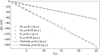 |
Fig. 5. Ionization potential lowering as a function of the effective charge in Fe II–Fe XXV and in O I–O VII. Solid line: fitting formula (9) for μ = 0.1 au. Dashed line: fitting formula (9) for μ = 0.25 au. Circles: MCDF/RATIP method, Fe II–Fe XXV for μ = 0.1 au. Squares: MCDF/RATIP method, Fe II–Fe XXV for μ = 0.25 au. Upright triangles: MCDF/RATIP method, O I–O VII for μ = 0.1 au. Downright triangles: MCDF/RATIP method, O I–O VII for μ = 0.25 au. |
 |
Fig. 6. K-threshold lowering as a function of the effective charge in Fe II–Fe XXV and in O I–O VII. Solid line: fitting formula (10) for μ = 0.1 au. Dashed line: fitting formula (10) for μ = 0.25 au. Circles: MCDF/RATIP method, Fe II–Fe XXV for μ = 0.1 au. Squares: MCDF/RATIP method, Fe II–Fe XXV for μ = 0.25 au. Upright triangles: MCDF/RATIP method, O I–O VII for μ = 0.1 au. Downright triangles: MCDF/RATIP method, O I–O VII for μ = 0.25 au. |
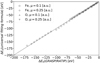 |
Fig. 7. Comparison between the ionization potential shifts obtained by the fitting formula (9) and those computed in this work for iron and oxygen ions. Dashed line: straight line of equality. Circles: Fe II–Fe XXV for μ = 0.1 au. Squares: Fe II–Fe XXV for μ = 0.25 au. Upright triangles: O I–O VII for μ = 0.1 au. Downright triangles: O I–O VII for μ = 0.25 au. |
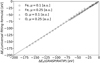 |
Fig. 8. Comparison between the K-threshold shifts obtained by the fitting formula (10) and those computed in this work for iron and oxygen ions. Dashed line: straight line of equality. Circles: Fe II–Fe XXV for μ = 0.1 au. Squares: Fe II–Fe XXV for μ = 0.25 au. Upright triangles: O I–O VII for μ = 0.1 au. Downright triangles: O I–O VII for μ = 0.25 au. |
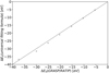 |
Fig. 9. Comparison between the ionization potential shifts obtained by the fitting formula (9) and those computed in this work for oxygen ions for μ = 0.2 au. Dashed line: straight line of equality. Circles: O I–O VII for μ = 0.2 au. |
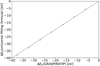 |
Fig. 10. Comparison between the K-threshold shifts obtained by the fitting formula (10) and those computed in this work for oxygen ions for μ = 0.2 au. Dashed line: straight line of equality. Circles: O I–O VII for μ = 0.2 au. |
The deviations between the fitted and computed values for all the iron and oxygen ions at the three plasma parameter values considered (μ = 0.1, 0.2, 0.25 au) vary 1–20% for the ionization potential lowering and 1–24% for the K-threshold shifts depending on the screening parameter. This is an important finding as it seems to indicate that the IP and K-threshold lowerings are practically independent of the atomic number Z. Hence, to a first approximation the fitting formulae (9) and (10) may be considered universal and readily applicable to other elements, thus simplifying the implementation of the continuum lowering corrections in XSTAR. However, more accurate fitting formulae could be clearly derived by considering each row of iron ions separately, although the slightly less accurate fitting formula we are proposing, which works reasonably well for all the ionization stages of iron (and oxygen), is more convenient. We also note that the fitting parameters appearing in the two formulae (9) and (10) could be improved by further MCDF/RATIP computations of IP and K-threshold lowerings in other elements of astrophysical interest.
5. Summary and conclusion
Following our previous analyses on the oxygen isonuclear sequence (Paper I) and on the highly (Paper II) and moderately (Paper III) charged Fe ions, here, we study the plasma environment effects on the atomic structure and decay parameters used to model the K lines of the lowly charged iron species Fe II–Fe VIII. The IPs, K-thresholds, wavelengths, radiative transition probabilities, and Auger widths have been calculated using the MCDF method simulating the plasma screening with a Debye–Hückel potential. In order to model typical plasma conditions encountered in black-hole and neutron-star accretion disks, we considered plasma screening parameter values ranging from μ = 0 au. to μ = 0.25 au. Our main results can be summarized as follows:
-
We confirm the linear behavior of both the IP and K threshold lowering with both the plasma screening parameter and the effective ionic charge and their close magnitude for each ionic species. Their values span from ∼ − 5 eV to ∼ − 60 eV.
-
K-line redshifts are small, 1–2 mÅ or less, among which the larger are for the Kβ lines.
-
The radiative rates and the Auger widths change only by a few percent and even less for most K lines.
-
Two universal fitting formulae are proposed for the threshold downshifts that depend only on the effective ionic charge and plasma screening parameter. They are expected to predict the IP and K-threshold shifts induced by the plasma environment for any elemental ion under the typical plasma conditions of the inner region of compact-object accretion disks.
In conclusion, we confirm that the high-resolution X-ray spectrometers onboard the future XRISM and ATHENA space missions will be able to detect the lowering of the K edges of these ions due to the extreme plasma conditions occurring in accretion disks around compact objects.
Acknowledgments
JD is Research Fellow of the Belgian Fund for Research Training in Industry and Agriculture (FRIA) while P.P. and P.Q. are, respectively, Research Associate and Research Director of the Belgian Fund for Scientific Research (F.R.S.-FNRS). Financial supports from these organizations, as well as from the NASA Astrophysics Research and Analysis Program (grant 80NSSC17K0345) are gratefully acknowledged. J.A.G. acknowledges support from the Alexander von Humboldt Foundation.
References
- Bautista, M. A., & Kallman, T. R. 2001, ApJS, 134, 139 [NASA ADS] [CrossRef] [Google Scholar]
- Beiersdorfer, P., Bitter, M., von Goeler, S., & Hill, K. W. 1989, Phys. Rev. A, 40, 150 [NASA ADS] [CrossRef] [Google Scholar]
- Crowley, B. J. B. 2014, High Energy Density Phys., 13, 84 [NASA ADS] [CrossRef] [Google Scholar]
- Decaux, V., Beiersdorfer, P., Osterheld, A., Chen, M., & Kahn, S. M. 1995, ApJ, 443, 464 [NASA ADS] [CrossRef] [Google Scholar]
- Deprince, J., Bautista, M. A., Fritzsche, S., et al. 2019a, A&A, 624, A74 [NASA ADS] [CrossRef] [EDP Sciences] [Google Scholar]
- Deprince, J., Bautista, M. A., Fritzsche, S., et al. 2019b, A&A, 626, A83 [NASA ADS] [CrossRef] [EDP Sciences] [Google Scholar]
- Deprince, J., Bautista, M. A., Fritzsche, S., et al. 2020, A&A, 635, A70 [CrossRef] [EDP Sciences] [Google Scholar]
- Djenize, S., Milosavljevic, V., & Sreckovic, A. 1998, J. Quant. Spectr. Rad. Transf., 59, 71 [NASA ADS] [CrossRef] [Google Scholar]
- Fabian, A. C., Rees, M. J., Stella, L., & White, N. E. 1989, MNRAS, 238, 729 [NASA ADS] [CrossRef] [Google Scholar]
- Fritzsche, S. 2012, Comput. Phys. Commun., 183, 1523 [NASA ADS] [CrossRef] [Google Scholar]
- García, J., & Kallman, T. R. 2010, ApJ, 718, 695 [NASA ADS] [CrossRef] [Google Scholar]
- García, J., Dauser, T., Lohfink, A., et al. 2014, ApJ, 782, 76 [NASA ADS] [CrossRef] [Google Scholar]
- Grant, I. P. 1988, Meth. Comput. Chem., 2, 1 [Google Scholar]
- Grant, I. P., McKenzie, B. J., Norrington, P. H., Mayers, D. F., & Pyper, N. C. 1980, Comput. Phys. Commun., 21, 207 [NASA ADS] [CrossRef] [Google Scholar]
- Hölzer, G., Fritsch, M., Deutsch, M., et al. 1997, Phys. Rev. A, 56, 4554 [NASA ADS] [CrossRef] [Google Scholar]
- Kallman, T. R., & Bautista, M. A. 2001, ApJS, 133, 221 [NASA ADS] [CrossRef] [Google Scholar]
- Khattak, F. Y., Percie du Sert, O. A. M. B., Rosmej, F. B., & Riley, D. 2012, J. Phys. Conf. Ser., 397, 012020 [CrossRef] [Google Scholar]
- Kramida, A., Ralchenko, Y., & Reader, J. NIST ASD Team 2019, NIST Atomic Spectra Database (version 5.7.1) (Gaithersburg, MD: National Institute of Standards and Technology), Available: http://physics.nist.gov/asd [2020, March 2] [Google Scholar]
- McKenzie, B. J., Grant, I. P., & Norrington, P. H. 1980, Comput. Phys. Commun., 21, 233 [NASA ADS] [CrossRef] [Google Scholar]
- Palmeri, P., Mendoza, C., Kallman, T. R., Bautista, M. A., & Meléndez, M. 2003, A&A, 410, 359 [NASA ADS] [CrossRef] [EDP Sciences] [Google Scholar]
- Parpia, F. A., Fischer, C. F., & Grant, I. P. 1996, Comput. Phys. Commun., 94, 249 [NASA ADS] [CrossRef] [Google Scholar]
- Reynolds, C. S. 2013, Class. Quant. Grav., 30, 244004 [NASA ADS] [CrossRef] [Google Scholar]
- Ross, R. R., & Fabian, A. C. 2005, MNRAS, 358, 211 [Google Scholar]
- Saha, B., & Fritzsche, S. 2006, Phys. Rev. E, 73, 036405 [NASA ADS] [CrossRef] [Google Scholar]
- Schnittman, J. D., Krolik, J. H., & Noble, S. C. 2013, ApJ, 769, 156 [NASA ADS] [CrossRef] [Google Scholar]
- Smith, R. K., & Brickhouse, N. S. 2014, Adv. At. Mol. Opt. Phys., 63, 271 [NASA ADS] [CrossRef] [Google Scholar]
- Sreckovic, A., Djenize, S., & Bukvic, S. 1996, Phys. Scr., 53, 54 [NASA ADS] [CrossRef] [Google Scholar]
- Stewart, J. C., & Pyatt, K. D., Jr 1966, ApJ, 144, 1203 [NASA ADS] [CrossRef] [Google Scholar]
All Tables
Reference configurations used to build up the MCDF active space (AS) listing the total number of configuration state functions (CSFs), NCSF, generated for the MCDF expansions in Fe II–Fe VIII.
Computed ionization potentials for Fe II–Fe VIII as a function of the plasma screening parameter μ (au).
Computed K-thresholds for Fe II–Fe VIII as a function of the plasma screening parameter μ (au).
Wavelengths and transition probabilities for the K lines of Fe II–Fe VIII (2 ≤ Zeff ≤ 8) computed with plasma screening parameters μ = 0.0, 0.1, and 0.25 au.
Comparison with measured centroid wavelengths (Å) for the Kα1, 2 and Kβ unresolved transition arrays in Fe X and Fe II.
Plasma environment effects on the Auger widths of K-vacancy states in Fe II (Zeff = 2) and Fe VIII (Zeff = 8) computed with plasma screening parameters μ = 0.0, 0.1, and 0.25 au.
All Figures
|
Fig. 1. Ionization potential shifts in Fe IX–Fe XXV as a function of the plasma screening parameter μ. Squares: Fe II. Circles: Fe III. Upright triangles: Fe IV. Downright triangles: Fe V. Rightward triangles: Fe VI. Leftward triangles: Fe VII. Stars: Fe VIII. |
| In the text | |
|
Fig. 2. Ionization potential shifts in Fe IX–Fe XXV as a function of the effective charge Zeff = Z − N + 1. Squares: μ = 0.1 au. Circles: μ = 0.25 au. |
| In the text | |
|
Fig. 3. Ionization potential of Fe II–Fe XII as a function of the effective charge Zeff = Z − N + 1. Circles: μ = 0 au (isolated atom). Squares: μ = 0.1 au. Triangles: μ = 0.25 au. Stars: NIST (Kramida et al. 2019). |
| In the text | |
|
Fig. 4. K thresholds of Fe II–Fe XII as a function of the effective charge Zeff = Z − N + 1. Circles: μ = 0 au (isolated atom). Squares: μ = 0.1 au. Triangles: μ = 0.25 au. |
| In the text | |
|
Fig. 5. Ionization potential lowering as a function of the effective charge in Fe II–Fe XXV and in O I–O VII. Solid line: fitting formula (9) for μ = 0.1 au. Dashed line: fitting formula (9) for μ = 0.25 au. Circles: MCDF/RATIP method, Fe II–Fe XXV for μ = 0.1 au. Squares: MCDF/RATIP method, Fe II–Fe XXV for μ = 0.25 au. Upright triangles: MCDF/RATIP method, O I–O VII for μ = 0.1 au. Downright triangles: MCDF/RATIP method, O I–O VII for μ = 0.25 au. |
| In the text | |
|
Fig. 6. K-threshold lowering as a function of the effective charge in Fe II–Fe XXV and in O I–O VII. Solid line: fitting formula (10) for μ = 0.1 au. Dashed line: fitting formula (10) for μ = 0.25 au. Circles: MCDF/RATIP method, Fe II–Fe XXV for μ = 0.1 au. Squares: MCDF/RATIP method, Fe II–Fe XXV for μ = 0.25 au. Upright triangles: MCDF/RATIP method, O I–O VII for μ = 0.1 au. Downright triangles: MCDF/RATIP method, O I–O VII for μ = 0.25 au. |
| In the text | |
|
Fig. 7. Comparison between the ionization potential shifts obtained by the fitting formula (9) and those computed in this work for iron and oxygen ions. Dashed line: straight line of equality. Circles: Fe II–Fe XXV for μ = 0.1 au. Squares: Fe II–Fe XXV for μ = 0.25 au. Upright triangles: O I–O VII for μ = 0.1 au. Downright triangles: O I–O VII for μ = 0.25 au. |
| In the text | |
|
Fig. 8. Comparison between the K-threshold shifts obtained by the fitting formula (10) and those computed in this work for iron and oxygen ions. Dashed line: straight line of equality. Circles: Fe II–Fe XXV for μ = 0.1 au. Squares: Fe II–Fe XXV for μ = 0.25 au. Upright triangles: O I–O VII for μ = 0.1 au. Downright triangles: O I–O VII for μ = 0.25 au. |
| In the text | |
|
Fig. 9. Comparison between the ionization potential shifts obtained by the fitting formula (9) and those computed in this work for oxygen ions for μ = 0.2 au. Dashed line: straight line of equality. Circles: O I–O VII for μ = 0.2 au. |
| In the text | |
|
Fig. 10. Comparison between the K-threshold shifts obtained by the fitting formula (10) and those computed in this work for oxygen ions for μ = 0.2 au. Dashed line: straight line of equality. Circles: O I–O VII for μ = 0.2 au. |
| In the text | |
Current usage metrics show cumulative count of Article Views (full-text article views including HTML views, PDF and ePub downloads, according to the available data) and Abstracts Views on Vision4Press platform.
Data correspond to usage on the plateform after 2015. The current usage metrics is available 48-96 hours after online publication and is updated daily on week days.
Initial download of the metrics may take a while.