© ESO 2020

1. Introduction

Substantial progress has been made in the study of the Milky Way rotation curve thanks to the application of a novel range of methods. Inside the solar circle, the tangent-point method has been applied by measuring spectral profiles of the HI and CO line emissions (Burton & Gordon 1978). Another approach considers the radial velocity of an object, which requires that its distance be measured independently, for example, by trigonometric or spectroscopic determinations. For this purpose, there is a variety of objects that can be adopted, such as OB stars and their associated molecular clouds (Blitz et al. 1982), the thickness of the HI layer (Merrifield 1992), the red giant branch and red clump (Bovy et al. 2012; Huang et al. 2016), classical Cepheids (Pont et al. 1997; Mróz et al. 2019), and a number of others. Rotation velocities can also be determined by measuring proper motions: when these are provided by Very Long Baseline Interferometry (VLBI) techniques, the rotation curve can be determined with high accuracy (Honma et al. 2019). The combination of proper motions from USNO-B1 observations with the Two Micron All Sky Survey (2MASS) photometric data has also been used to determine the rotation curve (López-Corredoira 2014). A powerful tool for measuring the rotation curve of the Milky Way is the VLBI Experiment for Radio Astrometry (VERA), which uses trigonometric determinations of three-dimensional positions and velocities of individual maser sources (Reid et al. 2009; Honma et al. 2015).

An significant study was carried by Bhattacharjee et al. (2014) to construct the rotation curve of the Milky Way from ∼0.2 kpc to ∼200 kpc by using a variety of disk and non-disk tracers. In analysing the velocity anisotropy parameter, they also estimated a lower limit for the Milky Way mass. Their work was continued by Bajkova & Bobylev (2017), who combined circular velocities of masers at low distances with the rotation curve of Bhattacharjee et al. (2014) and fit the result using a number of models, varying, in particular, the dark matter halo, where they refine parameters for six different models. A comparison of some of our fit parameters with the results of Bajkova & Bobylev (2017) is given in Sect. 5. An excellent review of the current status of the study of the rotation curve of the Milky Way is given in Sofue (2020).

Today, the Gaia mission of the European Space Agency (Gaia Collaboration 2016) provides a new possibility for studying the Milky Way with unprecedented accuracy thanks to data that offers the most accurate information about our Galaxy to date. Indeed, the Gaia data offer very precise determinations of position, proper motions, radial velocity measurements, and distance for millions of stars, although the errors of distance measurements increase with the distance from the observer.

In this paper, we present a systematical analysis of the Milky Way rotation curves derived by means of different methods and by using the Second Data Release (DR2) of the Gaia mission (Gaia Collaboration 2018a). To calculate the rotation curve, we use the Jeans equation that relates the circular velocity to observational quantities, such as the Galactocentric radial and tangential velocities, along with their respective dispersions. To do so, we must assume that the gravitational potential of Milky Way is axisymmetric and that the Galaxy is in a steady state configuration. In addition, by using numerical N-body experiments of simple disk models, we try to quantify the effect of the deviations from the equilibrium configuration on the determination of the rotation curve through the Jeans equation.

This paper is organized as follows: in Sect. 2, we describe the selection of the data used in this paper and in Sect. 3, we illustrate the method used to measure the Milky Way’s rotation curve and present our determinations. In Sect. 4, we explain the method for calculating the density distribution from the Poisson equation by using the measured rotation curve. In Sect. 5, we fit different density models to our determination of the rotation curve using standard dark matter approaches, that is, by assuming that the Galaxy is embedded in a quasi-spherical halo whose mass can be then derived on the basis of such an hypothesis. In Sect. 6, we present our density models based on the Modified Newtonian Dynamics (MOND) theory. We study in Sect. 7 the deviations from the Jeans equation in out-of-equilibrium systems. Finally, in Sect. 8, we present our conclusions.

2. Data selection

López-Corredoira & Sylos-Labini (2019, hereafter LS19) have produced extended kinematic maps of the Milky Way by using data from the second Gaia data release DR2 (Gaia Collaboration 2018a) and considering stars with measured radial heliocentric velocities and with parallax error less than 100%. Their total sample contains 7 103 123 sources. Such objects were observed by the Radial Velocity Spectrometer (RVS, Cropper et al. 2018), which collects medium-resolution spectra (spectral resolution $\frac{\lambda }{\mathrm{\Delta }\lambda }\approx 11700$) over the wavelength range of 845–872 nm, centred on the Calcium triplet region. Radial velocities are averaged over a 22-month observational time span. Most sources have a magnitude brighter than 13 in the G filter.

As the parallax error grows with the distance from the observer, LS19 applied a statistical deconvolution of the parallax errors based on the Lucy’s inversion method (Lucy 1974) to statistically estimate the distance. In this way, they derived the extended kinematical maps in the range of Galactocentric distances up to 20 kpc. We chose this method due to its advantage over other Bayesian methods (e.g. Astraatmadja & Bailer-Jones 2016; Bailer-Jones et al. 2018) as it does not assume any priors about the Milky Way density distribution. Any other method, such as the Lutz-Kelker method (Lutz & Kelker 1973), is not appropriate here since it would assume a uniform stellar volume density and a constant ratio σ_π/π, where π is the observed parallax and σ_π its standard deviation. For more details on this topic, see Luri et al. (2018), which gives an extensive analysis of different methods if inferring distance from the parallax, along with their respective advantages and disadvantages.

In further detail, the effective temperatures for the sources with radial velocities that LS19 considered are in the range of 3550 to 6900 K. The uncertainties of the radial velocities are: 0.3 km s⁻¹ at G_RVS <  8, 0.6 km s⁻¹ at G_RVS = 10, and 1.8 km s⁻¹ at G_RVS = 11.75; along with systematic radial velocity errors of < 0.1 km s⁻¹ at G_RVS <  9 and 0.5 km s⁻¹ at G_RVS = 11.75. The uncertainties of the parallax are: 0.02–0.04 mas at G <  15, 0.1 mas at G = 17, 0.7 mas at G = 20 and 2 mas at G = 21. The uncertainties of the proper motion are: 0.07 mas yr⁻¹ at G <  15, 0.2 mas yr⁻¹ at G = 17, 1.2 mas yr⁻¹ at G = 20 and 3 mas yr⁻¹ at G = 21. For details on radial velocity data processing and the properties and validation of the resulting radial velocity catalogue, see Sartoretti et al. (2018) and Katz et al. (2019). The set of standard stars that was used to define the zero-point of the RVS radial velocities is described in Soubiran et al. (2018). LS19 consider the zero-point bias in the parallaxes of Gaia DR2, as found by Lindegren et al. (2018), Arenou et al. (2018), Stassun & Torres (2018), Zinn et al. (2019); however, they find that the effect of the systematic error in the parallaxes is negligible, so the maps that we use from their study (LS19, Figs. 8–12) do not consider the zero-point correction. We describe the way we use these maps in Sect. 3 to construct the rotation curves (Fig. 1), however, in Fig. 2, we include the zero-point correction to demonstrate that the difference is negligible.

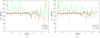Fig. 1. Panel a: rotation curves at different heights for positive values of z. Panel b: rotation curves at different heights for negative values of z. The error bars represent the standard deviation.

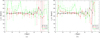Fig. 2. Rotation curves for different values of z including the zero point correction in parallax. Panel a: rotation curves at different heights for positive values of z. Panel b: rotation curves at different heights for negative values of z. The error bars represent the standard deviation.

3. Rotation curves

From the Gaia DR2 catalogue, we estimate, for each object, the parallax π, the Galactic coordinates (l, b), the radial velocity v_r, and two proper motions in equatorial coordinates μ_a cos δ and μ_δ. For our analysis, we need to know the Galactocentric position of stars in cylindrical coordinates (R, z, Φ), and the Galactocentric velocity in cylindrical coordinates (v_R, v_Φ, v_z). The transformation from these two coordinates systems can be found in LS19.

We limit the range of vertical distance to |z| < 2.2 kpc as we find that far off-plane data are affected by larger errors in their parallax determinations. We investigate the disk beyond the solar Galactocentric radius, that is, for 8.4 kpc< R <  21.2 kpc.

To determine the rotation curve, we consider the one component of Jeans equations in cylindrical coordinates (Binney & Tremaine 1987, Ch. 4.2, 4–29a):

$$\begin{array}{c}\hfill \frac{\partial (\nu \overline{v_{\mathrm{R}}})}{\partial t}+\nu (\frac{\overline{v_{\mathrm{R}}^2}-\overline{v_{\mathrm{\Phi }}^2}}{R}+\frac{\partial \mathrm{\Phi }}{\partial R})+\frac{\partial (\nu \overline{v_{\mathrm{R}}^2})}{\partial R}+\frac{\partial (\nu \overline{v_{\mathrm{R}}{v}_{\mathrm{Z}}})}{\partial z}=0,\end{array}$$(1)

where R is the Galactocentric radius, v_R is the radial velocity, v_Z is the vertical velocity, v_Φ is the azimuthal velocity, and ν is the volume density. The quantity $\overline{v^2}$ is the average square velocity for each component that can be written as $\overline{v^2}={\sigma }^2+{\overline{v}}^2$, where σ is the velocity dispersion. For a detailed calculation of the velocities and their respective dispersion, see LS19.

The rotational velocity is defined as (Binney & Tremaine 1987)

$$\begin{array}{c}\hfill v_c^2(R,z)=R\frac{\partial \mathrm{\Phi }}{\partial R}.\end{array}$$(2)

We use the standard assumption that the volume density can be written as

$$\begin{array}{c}\hfill \nu (R,z)={\rho }_0{e}^{-\frac{R}{h_R}}{e}^{-\frac{|z|}{h_z}},\end{array}$$(3)

where h_R is the scale length and h_z is the scale height. From Eqs. (1)–(3) we obtain the rotational velocity as function of R, z, that is, the rotation curves,

$$\begin{array}{cc}\hfill v_c^2& ={\overline{v_{\mathrm{\Phi }}}}^2+{\sigma }_{\mathrm{\Phi }}^2+({\overline{v_{\mathrm{R}}}}^2+{\sigma }_R^2)\frac{R-h_{\mathrm{R}}}{h_{\mathrm{R}}}-2R\overline{v_{\mathrm{R}}}\frac{\partial \overline{v_{\mathrm{R}}}}{\partial R}\hfill \\ \hfill & -R\frac{\partial {\sigma }_R^2}{\partial R}+\frac{R}{h_z}\frac{z}{|z|}\overline{v_{\mathrm{R}}{v}_{\mathrm{z}}}-R\frac{\partial (\overline{v_{\mathrm{R}}{v}_{\mathrm{z}}})}{\partial z}·\hfill \end{array}$$(4)

We determined the rotation curves for different values of z, in the direction of the anti-center, in bins of size ΔR = 0.5 kpc and Δz = 0.2 kpc. For what concerns the scale parameters in Eq. (3), we chose values of h_R = 2.5 kpc and h_z = 0.3 kpc (Jurić et al. 2008). Figure 1 shows the results of our fit.

Figure 2 shows the rotation curves, including the zero-point correction in parallax. The difference from the rotation curves in Fig. 1 is negligible and we do not consider this correction for the rest of the analysis. The results for different scale parameters are almost identical, as we show in Fig. 3. We observe a flat rotation curve, although it does exhibit some fluctuations. Our rotation curve in the plane of the Galaxy has a small positive gradient of 0.54 ± 0.7(stat.)±0.5(syst.) km s⁻¹ kpc⁻¹. Recent results have shown an opposite trend: Eilers et al. (2019) measured rotation curve for Galactocentric distances 5 kpc  ≤ R ≤ 25 kpc by combining spectral data from the Apache Point Observatory Galactic Evolution Experiment (APOGEE, Majewski et al. 2017) and photometric information from Wide-field Infrared Survey Explorer (WISE, Wright et al. 2010), 2MASS (Skrutskie et al. 2006), and Gaia DR2, finding a rotation curve with a declining slope of −1.7 ± 0.1 km s⁻¹ kpc⁻¹, with a systematic uncertainty of 0.46 km s⁻¹ kpc⁻¹. A similar result was obtained by Mróz et al. (2019), who used classical Cepheids to obtain the rotation curve of the Milky Way for Galactocentric distances 4 kpc  ≲ R ≲ 20 kpc, finding a rotation curve with a small negative slope of −1.34 ± 0.21 km s⁻¹ kpc⁻¹. Bhattacharjee et al. (2014) have also used the Jeans equation, but only for large distances (R >  20 kpc), which we do not consider in our analysis. For the disk tracers, they use the tangent point method for small distances and for higher distances they assume that the tracers follow nearly circular orbit. The advantage is that their method is independent from any density model, although it strongly depends on values of Galactic constants (Sun’s distance from, and circular rotation speed around, the Galactic centre). Nevertheless, their results for rotation curve for various values of Galactic constants are consistent with our findings. We discuss these results more in detail in what follows.

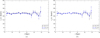Fig. 3. Rotation curves for different values of the scale parameters. Panel a: rotation curves for different values of hR, for z = 0. Panel b: rotation curves for different values of hz, for z = 0. The error bars represent the standard deviation.

4. Density distribution from the Poisson equation

Based on the results obtained for the rotation curve, we proceed to determine the density distribution in the Milky Way by considering different approaches. The first one is based on the Poisson equation in cylindrical coordinates and it assumes the dependence of the rotation speed with the azimuth to be negligible:

$$\begin{array}{c}\hfill \frac{1}{R}\frac{\partial }{\partial R}\left(R\frac{\partial \mathrm{\Phi }}{\partial R}\right)+\frac{{\partial }^2\mathrm{\Phi }}{\partial z^2}=4\pi G\rho (R,z)·\end{array}$$(5)

The first term on left side can be easily obtained by using Eq. (2). The second term, on the left side, can be obtained with the same relation and switching derivatives

$$\begin{array}{cc}\hfill \frac{{\partial }^2}{\partial z^2}\left(\frac{\partial \mathrm{\Phi }}{\partial R}\right)& =\frac{1}{R}\frac{{\partial }^2{v}_c^2}{\partial z^2},\hfill \\ \hfill \frac{\partial }{\partial R}\left(\frac{{\partial }^2\mathrm{\Phi }}{\partial z^2}\right)& =\frac{1}{R}\frac{{\partial }^2{v}_c^2}{\partial z^2}·\hfill \end{array}$$

By integrating the latter relation we find

$$\begin{array}{c}\hfill \frac{{\partial }^2\mathrm{\Phi }}{\partial z^2}=-{\displaystyle {\int }_R^{R_{\max }}\frac{1}{R}\frac{{\partial }^2{v}_c^2}{\partial z^2}\mathrm{d}R+\mathrm{\Phi }(R_{\max },z=0)·}\end{array}$$(6)

To determine derivatives of v_c with respect to R, z, we assume that $v_c^2$ has a linear behaviour of the type

$$\begin{array}{c}\hfill v_c^2=a(z)(R-14)+b(z),\end{array}$$(7)

where clearly a(z) and b(z) must be determined from the data. We find that a(z) and b(z) can be nicely fitted by parabolas and therefore, we can write

$$\begin{array}{c}\hfill v_c^2(z)=[(\alpha +\beta z^2)+(\gamma +\delta z^2)(R-14)],\end{array}$$(8)

where the numerical values of α, β, γ, δ are estimated from the data and the values are given below. We use Eqs. (2) and (7) to express the first term of Eq. (5) as

$$\begin{array}{cc}\hfill \frac{1}{R}\frac{\partial }{\partial R}\left(R\frac{\partial \mathrm{\Phi }}{\partial R}\right)& =\frac{1}{R}\frac{\partial }{\partial R}(a(z)(R-14)+b(z))\hfill \\ \hfill & =\frac{a(z)}{R}\hfill \end{array}$$(9)

By making the derivative of the fit of the rotational velocity (Eq. (8)) with respect to z, we express Eq. (6) as

$$\begin{array}{cc}\hfill \frac{{\partial }^2\mathrm{\Phi }}{\partial z^2}& =2\beta \ln \left(\frac{R}{R_{\max }}\right)+2\delta (R-R_{\max })\hfill \\ \hfill & -28\delta \ln \left(\frac{R}{R_{\max }}\right)+\mathrm{\Phi }(R_{\max },z=0).\hfill \end{array}$$(10)

We find that the best fit values for a(z) and b(z) are (see Fig. 4):

$$\begin{array}{cc}\hfill a(z)& =(-2200\pm 400)z^2+(1000\pm 1000)\hfill \\ \hfill b(z)& =(11400\pm 1000)z^2+(53000\pm 1500).\hfill \end{array}$$

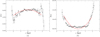Fig. 4. Panel a: fit of a(z). Panel b: fit of b(z) (see Eq. (8)). The error bars represent the standard deviation.

In the Galactic plane, the value of a(z) is positive, which means that in the plane the velocity gradient is positive too: this must be compensated by density increase. That is clearly non-physical as we know that in our Galaxy, the density decreases exponentially in the outwards direction. Therefore, we conclude that we cannot use the Poisson equation to determine the density analytically. This problem may be related to large fluctuations present in the data, as well as by the fact that the system is not in equilibrium, so it does not satisfy the assumptions of the Jeans equation. We analyse the effect of the deviations from equilibrium in greater detail in Sect. 7.

5. Density fit with the dark matter model

Another method to fit the rotation curve data can be done by making use of known density models. By assuming that the system is in equilibrium and made by different mass components, both the density and the rotational velocity can be expressed as

$$\begin{array}{cc}\hfill \rho & ={\rho }_{\mathrm{bulge}}+{\rho }_{\mathrm{disk}}+{\rho }_{\mathrm{halo}},\hfill \end{array}$$(11)

$$\begin{array}{cc}\hfill v_c^2& =v_{c,\mathrm{bulge}}^2+v_{c,\mathrm{disk}}^2+v_{c,\mathrm{halo}}^2,\hfill \end{array}$$(12)

that is, we have decomposed the density and the circular velocity as the sum of three terms: the bulge, the disk, and the halo. Here, we examine each of these terms in more detail.

We do not fit the bulge, as we are interested mainly in outer parts of disk, where contribution of the bulge is negligible: we use

$$\begin{array}{c}\hfill v_{c,\mathrm{bulge}}^2=\frac{G{M}_{\mathrm{bulge}}}{R},\end{array}$$(13)

where M_bulge = 2 × 10¹⁰ M_⊙ (Valenti et al. 2016).

For the disk, by assuming the balance between the gravitational and centrifugal forces at a generic point (r, ϕ, h) (for a detailed derivation see Appendix A) we derive:

$$\begin{array}{cc}& {\displaystyle {\int }_{-H/2}^{H/2}{\int }_{R_{\min }}^{R_{\max }}\frac{2}{r}[\frac{(\widehat{r}+r)(\widehat{r}-r)+\mathrm{\Delta }{h}^2}{[{(\widehat{r}-r)}^2+\mathrm{\Delta }{h}^2]\sqrt{{(\widehat{r}+r)}^2+\mathrm{\Delta }{h}^2}}E(k)}\hfill \\ \hfill & -\frac{1}{\sqrt{{(\widehat{r}+r)}^2+\mathrm{\Delta }{h}^2}}K(k)]\nu (\widehat{r},\widehat{h})\mathrm{d}\widehat{r}\mathrm{d}\widehat{h}\hfill \\ \hfill & +A\frac{v_{c,\mathrm{disk}}{(r,h)}^2}{r}=0,\hfill \end{array}$$(14)

where K(k),E(k) are complete elliptic integrals of the first and second kind respectively, and

$$\begin{array}{c}\hfill k^2=\frac{4\widehat{r}r}{{(\widehat{r}+r)}^2+\mathrm{\Delta }{h}^2},\end{array}$$(15)

where $\mathrm{\Delta }{h}^2={(\widehat{h}-h)}^2$. For the sake of simplicity, we consider only a thin disk and we approximate Δh ≈ h. For the density in Eq. (14) we used the relation:

$$\begin{array}{c}\hfill \nu (\widehat{r},\widehat{z})={\rho }_0{e}^{-\widehat{r}/h_R}{e}^{-|\widehat{h}|/h_z}.\end{array}$$(16)

In Eq. (14) the constant A is the Galactic rotation number defined as

$$\begin{array}{c}\hfill A=\frac{R_{g,\max }{V}_0^2}{G{M}_{d,\max }},\end{array}$$(17)

where M_d, max is mass of the disk, for which we use the value M_d, max = 6.5 × 10¹⁰ M_⊙ (Sofue et al. 2013). R_g, max is the radius of the disk, which we fix at 25 kpc, V₀ is the maximum velocity corresponding to the flat part of the rotation curve in the data-set: 257 km s⁻¹ in our case and G is the gravitational constant: 4.302 × 10⁻⁶ kpc $M_{\odot }^{-1}$ (km s)⁻². We calculate the fit in the Galactic plane, where Δh → 0 and Eq. (14) becomes

$$\begin{array}{cc}& {\displaystyle {\int }_{R_{\min }}^{R_{\max }}[\frac{E(k)}{\widehat{r}-r}-\frac{K(k)}{\widehat{r}+r}]{\rho }_0{e}^{-\widehat{r}/h_R}\widehat{r}\mathrm{d}\widehat{r}+A\frac{v_{c,\mathrm{disk}}{(r)}^2}{2|h|}=0,}\hfill \end{array}$$(18)

where

$$\begin{array}{c}\hfill k^2=\frac{4r\widehat{r}}{{(\widehat{r}+r)}^2}.\end{array}$$(19)

To fit the dark matter halo, we assume this is well approximated by the so-called Navarro, Frenk, and White density profile (Navarro et al. 1997)

$$\begin{array}{cc}\hfill {\rho }_{\mathrm{halo}}& =\frac{{\rho }_{0h}}{\frac{R}{R_s}{(1+\frac{R}{R_s})}^2},\hfill \end{array}$$(20)

$$\begin{array}{cc}\hfill v_{c,\mathrm{halo}}^2(R)& =\frac{4\pi G{\rho }_{0h}{R}_s^3}{R}[log\left(\frac{R_s+R}{R_s}\right)-\frac{R}{R_s+R}].\hfill \end{array}$$(21)

We use the least-squares method to find the best values of the free parameters. As this method requires a long computational time, we fix some well-known parameters and only fit those that are not so well determined. First, we fit only data in the Galactic plane, where we fix h_R = 2.5 kpc and R_s = 14.8 kpc, which are the values found by Eilers et al. (2019). For the free parameters, we obtain the values ρ_0h = 2 × 10⁷ M_⊙ kpc⁻³ and ρ₀ = 3.83 × 10⁸ M_⊙ kpc⁻³, with the value of the minimal χ² = 15.424 for 107 points. We plot this result in Fig. 5a. We see that our rotation curves are well explained by a dominant dark matter halo, with a minimal contribution from the disc. From these values, we calculate the mass of the dark matter halo up to 25 kpc to be M_h = 3.52 × 10¹¹ M_⊙, which is smaller than 7.25 × 10¹¹ M_⊙ found by Eilers et al. (2019), but higher than 2.9 × 10¹¹ M_⊙ found by Bajkova & Bobylev (2017). For the disk, we find M_d = 1.41 × 10¹⁰ M_⊙, which is lower than values found in the literature, for example, 6.5 × 10¹⁰ M_⊙ as found by Sofue et al. (2009), 0.95 × 10¹¹ M_⊙ as found by Kafle et al. (2014), or 6.51 × 10¹⁰ M_⊙ as found by Bajkova & Bobylev (2017).

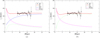Fig. 5. Fit of the rotation curve for only z = 0 using dark matter (left) and the MOND theory (right). The data are binned with bins of size ΔR = 0.5 kpc and Δz = 0.1 kpc. (a) Dark matter, (b) MOND.

For the off-plane data, we fit rotation curves for different values of z at the same time, using relation (14), which adds one more free parameter h_z to the fit. Again, to save computational time, we restricted the number of free parameters and fixed h_R = 2.5 kpc and R_s = 14.8 kpc. We find h_z = 0.3 kpc, ρ₀ = 4.1 × 10⁹ M_⊙ kpc⁻³ and ρ_0h = 2.389 × 10⁷ M_⊙ kpc⁻³, with the value of minimal χ² = 2510.37 for 4653 points. In Fig. 6, we plot the fit for various values of z. We see that in all cases, the dark matter halo is strongly dominant and the contribution from the disk is less important, which is as expected from rotational velocity that does not change with vertical distance.

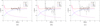Fig. 6. Fit of the rotation curve for various values of z using dark matter model. The data is binned with bins of size ΔR = 0.5 kpc and Δz = 0.1 kpc. (a) z = 0 kpc, (b) z = 1.0 kpc, (c) z= −1.0 kpc.

This result is in agreement with result of Eilers et al. (2019), who also fitted their rotation curve with a similar model. They also find a dominant dark matter halo, with free parameter ρ_0h = 1.06 × 10⁷ M_⊙ kpc⁻³. However, we disagree with result from Jałocha et al. (2010), who found that the gross mass distribution in our Galaxy is disk-like, without the need for a halo. Jałocha et al. (2010) obtained their result based on modelling vertical gradient of azimuthal velocity, assuming the quasi-circular orbit approximation, and relating v_c to v_ϕ directly from the balance condition of the radial component of gravitational and inertial force. We guess that the difference between our results comes from the fact that Jałocha et al. (2010) did not take the Jeans equations into account when deriving rotational velocity. Indeed, in this latter work, assuming quasi-circular orbits v_ϕ was directly related to v_c to obtain $v_{\varphi }=\frac{r}{R}{v}_c$.

6. Density fit with the MOND model

We tried to fit our results using the MOND theory, without invoking the presence of a heavy dark matter halo. To this purpose we have recalculated the expressions for the disk and the bulge, using relations from MOND (Milgrom 1983):

$$\begin{array}{c}\hfill a_M=\frac{a_N}{\mu (\frac{a_M}{a_0})},\end{array}$$(22)

where

$$\begin{array}{c}\hfill \mu \left(\frac{a_M}{a_0}\right)=\sqrt{\frac{1}{1+{\left(\frac{a_0}{a_M}\right)}^2}},\end{array}$$(23)

with the value of a₀ = 1.2 × 10⁻¹⁰ ms⁻² (Scarpa et al. 2006). Solving Eq. (22) analytically yields

$$\begin{array}{c}\hfill a_M=\sqrt{\frac{1}{2}{a}_N^2+\sqrt{\frac{1}{4}{a}_N^4+a_N^2{a}_0^2}}.\end{array}$$(24)

Equation (22) is indeed an approximation, which does not exactly stray from a spherical symmetric mass distribution. The exact solution may be analysed in the context for Bekenstein-Milgrom MOND theory derived from the modification of classical Newtonian dynamics (Brada & Milgrom 1995). However, the difference between the approximation of Eq. (22) and the exact solution is small, so we neglect it here.

For the fit, we only used the disk and the bulge components. In Fig. 5b, we plot the result of the fit for the Galactic plane, nicely matching the observed value. For the free parameters, we found ρ₀ = 7.49 × 10⁸ M_⊙ kpc⁻³ and h_R = 4.8 kpc. The values of minimal χ² is χ² = 15.776 for 107 points, which is similar to the value for Newtonian fit. The mass of the disk up to 25 kpc found with these parameters is M_d = 2.77 × 10¹⁰ M_⊙ which is almost two times higher than that obtained with the dark matter model.

We tried to fit the off-plane rotation curve with the same approach. Again, we fit data for all z with models for all z at the same time. Thus, we find: ρ₀ = 9.15 × 10⁹ M_⊙ kpc⁻³ and h_R = 5.0 kpc. We fixed the value of scale-height to h_z = 0.3 kpc. The obtained value of minimal χ² = 2677.58 for 4653 points, which is comparable with the Newtonian case. In Fig. 7, we plot the results of the fit with MOND for different values of z. We see that off-plane, the fit is satisfying and there is no preference for the dark matter model over the MOND model. However, our result contradicts that of Lisanti et al. (2019), who also used Milky Way observables to compare the differences between dark matter and MOND theories. They performed a Bayesian likelihood analysis to compare the predictions of the model with the observed quantities. They find that the dark matter model is preferred, as MOND-like theories struggle to simultaneously explain both the rotational velocity and vertical motion of nearby stars in the Milky Way.

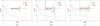Fig. 7. Fit of the rotation curve for various values of z using the MOND theory. The data are binned with bins of size ΔR = 0.5 kpc and Δz = 0.1 kpc. (a) z = 0 kpc, (b) z = 1.0 kpc, (c) z = −1.0 kpc.

7. Corrections to the Jeans equation

So far, we used the Jeans equation to determine the rotation curve of the Milky Way and its density profile. We recall that the basic assumptions of the Jeans equation are that the system is collisionless, axisymmetric, and in equilibrium. While the first condition represents a reasonable working hypothesis since collisional effects take place on much longer time scales than those that astrophysically relevant, the recent Gaia data have shown that the Milky Way is not in a stationary situation as there are large-scale gradients in all components of the velocity field and there are clear deviations from axisymmetry (Gaia Collaboration 2018b; Wang et al. 2018; López-Corredoira & Sylos-Labini 2019; Wang et al. 2020). The dynamical origin of such features represents an open problem that has been explored by several authors (Antoja et al. 2018; Binney & Schönrich 2018). For instance, it has been concluded that the Galactic disk is still dynamically young and was last perturbed less than 1 Gyr ago, therefore modelling it as axisymmetric and in equilibrium is incorrect (Antoja et al. 2018). The problem of reliability with regard to the Jeans equation was also studied by Haines et al. (2019), who analysed an N-body simulation of a stellar disk which had been perturbed by the recent passage of a dwarf galaxy and studied the surface density of the system based on the Jeans equation. They found that the Jeans equation gives reasonable results in over-dense regions, but fails in under-dense regions. Thus, the development of non-equilibrium methods for estimating the dynamical matter density locally and in the outer disk is necessary.

In order to test the effects of the deviations from a stationary configuration and axisymmetry on the Jeans equation, we consider N-body simulations of mock galactic systems that are not completely in an equilibrium configuration. The evolution of these systems was discussed in details in Benhaiem et al. (2017, 2019); Sylos Labini et al. (in prep.). We consider, hereafter, one of these systems, consisting of a thin, rotating, self-gravitating disk embedded in an ellipsoidal dark matter halo with an isotropic velocity dispersion. The inner regions of this system are very close to a stationary configuration, while the outer regions are progressively out-of-equilibrium. The signature of such a situation is represented by the behaviour of the radial velocity averaged in shells: at small distances from the centre this is close to zero, while at large enough distances, it becomes positive: the amplitude grows with the distance from the centre.

The circular velocity from the Jeans equation is

$$\begin{array}{c}\hfill v_{c,J}^2={\overline{v_{\mathrm{\Phi }}}}^2-{\overline{v_{\mathrm{R}}}}^2(1+\frac{\partial \ln \nu }{\partial \ln R}+\frac{\partial \ln {\overline{v_{\mathrm{R}}}}^2}{\partial \ln R}),\end{array}$$(25)

where we neglect the cross-term $\overline{v_R{v}_{\varphi }}$, as it’s contribution to the final result is negligible ( ∼ 1%) (Eilers et al. 2019). By definition, the circular velocity can be computed from the gravitational force:

$$\begin{array}{c}\hfill v_{c,F}^2=R{F}_R=|\overline{\mathit{F}}·\mathit{R}|,\end{array}$$(26)

where $\overline{\mathit{F}}$ is the gravitational force acting of the particles contained in the two-dimensional corona at a distance, R, and thickness, ΔR (where R is the cylindrical coordinate). Thus, we compute the gravitational force acting of the ith particle as

$$\begin{array}{c}\hfill {\mathit{F}}_i=G{\displaystyle \sum _{j=1}^N}{m}_j{m}_i\frac{({\mathit{r}}_i-{\mathit{r}}_j)}{|{\mathit{r}}_i-{\mathit{r}}_j{|}^3},\end{array}$$(27)

where m_i is the mass of the ith particle and we compute its average in a corona. If axisymmetry and stationary equilibrium are established, then v_c, F = v_c, J: the difference between these two quantities thus depends on the deviations from the assumptions underlying the Jeans equation. In the Fig. 8, we plot the ratio:

$$\begin{array}{c}\hfill \mathrm{\Theta }=\frac{v_{c,J}}{v_{c,F}}\end{array}$$(28)

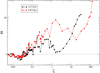Fig. 8. Ratio of the circular velocity from the Jeans equation and from the force (i.e. Eq. (28)) as a function of the ratio between the average radial velocity and the azimuthal velocity (see Eq. (29)). Black and red circles correspond to the system evolved up to 3/9 Gyr, respectively.

as a function of

$$\begin{array}{c}\hfill \zeta =\frac{|v_R|}{|v_{\varphi }|}·\end{array}$$(29)

When the radial velocity is small, that is, ζ ≪ 1, then Θ ≈ 1, whereas when the radial velocity becomes larger than 10% of the azimuthal one, then Θ becomes larger than one. In the Milky Way, ζ ≈ 0.1 at R ≈ 20 kpc, as found by LS19. We note that in Fig. 8, we have reported the behaviour for two different times, that is, 3 and 9 Gyr; indeed, as the external regions are out-of-equilibrium they continue to evolve over time, while the inner regions are quasi stationary.

We conclude that the Jeans equation is reliable when the radial velocity is smaller than 10% of the azimuthal one, otherwise corrections to the Jeans equation become necessary. In particular, we find that the estimation of the circular velocity though the Jeans equation gives an overestimation with respect to the estimation of the circular velocity through the force. This implies that by using v_c, J to compute the mass through the relation,

$$\begin{array}{c}\hfill M_J(r)=\frac{v_{c,J}^2\times r}{G},\end{array}$$(30)

the real mass is overestimated by a factor that is proportional to Θ².

8. Conclusions

In this paper, we study the rotation curve of the Milky Way from the extended kinematic maps of Gaia-DR2. We calculated the rotation curve in plane and in off-plane regions, using the Jeans equation. Our results show that the rotation curve in the outer disk has very little dependence on R and z.

We fitted the rotation curve using models with dark matter halo or MOND, using the least-squares method. We find that a model based on dark matter fits the data very well, and the results are in good agreement with other works. For the dark matter model, we obtain the minimal χ² = 15.424 for 107 points in the plane and χ² = 2510.37 for 4653 points off plane. The MOND model in the plane gives χ² = 15.776 for 107 points, which is comparable with the dark matter model. Off-plane the results are similar as well, with χ² = 2677.58 for 4653 points, which fits the data similarly to the dark matter model.

We also considered the corrections to the Jeans equation in non-equilibrium and non-axisymmetric systems. Indeed, the Jeans equation assumes that the system is axisymmetric and in equilibrium, which is not the case of the Milky Way. For this reason, we consider N-body simulations of galaxies and calculated the rotational velocity by using the Jeans equation v_c, J and by computing the gradient of the gravitational potential v_c, F. We find that the two ways of calculating the rotational velocity are in good agreement as long as the ratio, ζ, between the modulus of the radial velocity and of the azimuthal velocity is smaller than ∼10%. When ζ becomes larger than this value, then v_c, J >  v_c, F and, thus, we overestimate the Galactic mass if we use the rotational velocity computed through the Jeans equation. For the case of the Milky Way, it was found in LS19 that ζ ≈ 0.1 at R ≈ 20 kpc: this implies that at a larger galactocentric distance, using the Jeans equation leads to an overestimation the mass of the Milky Way. The Gaia DR3 will clarify whether in the range of distances 20 <  R <  30 kpc, such corrections may become large enough to change our view of the Galaxy as a quasi-equilibrium system, thus altering its estimated mass.

Acknowledgments

We thank the anonymous referee for helpful comments, which improved this paper and Agnes Monod-Gayraud (language editor of A&A) for proof-reading of the text. ZC and MLC were supported by the grant PGC-2018-102249-B-100 of the Spanish Ministry of Economy and Competitiveness (MINECO). HFW is supported by the LAMOST Fellow project, National Key Basic R&D Program of China via 2019YFA0405500 and funded by China Postdoctoral Science Foundation via grant 2019M653504, Yunnan province postdoctoral Directed culture Foundation and the Cultivation Project for LAMOST Scientific Payoff and Research Achievement of CAMS-CAS. RN was supported by the Scientific Grant Agency VEGA No. 1/0911/17. This work has made use of data from the European Space Agency (ESA) mission Gaia (https://www.cosmos.esa.int/gaia), processed by the Gaia Data Processing and Analysis Consortium (DPAC, https://www.cosmos.esa.int/web/gaia/dpac/consortium). Funding for the DPAC has been provided by national institutions, in particular the institutions participating in the Gaia Multilateral Agreement.

References

Appendix A: Derivation of the integral of the thin disk

To derive the rotation curve of a disk in 3D, we derive the equation for balance between the gravitational and the centrifugal force. We consider two points with the coordinates P(r, θ, z) and $Q(\widehat{r},\widehat{\theta },\widehat{z})$. The distance between these two points can be expressed as ${({\widehat{r}}^2-r^2-2r\widehat{r}cos\widehat{\theta }+\mathrm{\Delta }{h}^2)}^{1/2}$ and the vector projection as $(\widehat{r}cos\widehat{\theta }-r)$, where Δh is the difference in heights $\mathrm{\Delta }h=(\widehat{h}-h)$. The Newtonian gravitational force on the point P from a body consisting of points Q distributed with a mass density $\widehat{\rho }(\widehat{r},\widehat{h})$ can be expressed as an integral over these points:

$$\begin{array}{cc}\hfill F_X& ={\displaystyle \frac{G{M}_{\mathrm{g}}}{R_{\mathrm{g}}^2}}{\displaystyle {\int }_{-H/2}^{H/2}{\int }_0^{2\pi }{\int }_0^1{\displaystyle \frac{\widehat{r}cos\widehat{\theta }-r}{{({\widehat{r}}^2+r^2-2\widehat{r}rcos\widehat{\theta }+\mathrm{\Delta }{h}^2)}^{3/2}}}}\hfill \\ \hfill & ·\widehat{\rho }(\widehat{r},\widehat{h})\widehat{r}\mathrm{d}\widehat{r}\mathrm{d}\widehat{\theta }\mathrm{d}\widehat{h}.\hfill \end{array}$$(A.1)

The centrifugal force can be written simply as

$$\begin{array}{c}\hfill F_c={\displaystyle \frac{V^2}{R}}={\displaystyle \frac{V_0^2}{R_{\mathrm{g}}}}{\displaystyle \frac{v{(r,h)}^2}{r}}·\end{array}$$(A.2)

Here, we made all the variables dimensionless by measuring the distances in units of the outermost galactic radius R_g, mass density $\widehat{\rho }$ in units of $M_{\text{g}}/R_{\text{g}}^3$, where M_g is the total galactic mass and velocities in units of the characteristic velocity V₀. So the balance between the gravitational and centrifugal force yields

$$\begin{array}{cc}& {\displaystyle {\int }_{-H/2}^{H/2}{\int }_0^{2\pi }{\int }_0^1\frac{\widehat{r}cos\widehat{\theta }-r}{{({\widehat{r}}^2-r^2-2r\widehat{r}cos\widehat{\theta }+\mathrm{\Delta }{h}^2)}^{3/2}}\widehat{\rho }(\widehat{r},\widehat{h})\widehat{r}\mathrm{d}\widehat{r}\mathrm{d}\widehat{\theta }\mathrm{d}\widehat{h}}\hfill \\ \hfill & +A\frac{v{(r,h)}^2}{r}=0,\hfill \end{array}$$(A.3)

where A is the galactic rotation number

$$\begin{array}{c}\hfill A=\frac{R_{\mathrm{g}}{V}_0^2}{G{M}_{\mathrm{g}}}·\end{array}$$(A.4)

We get rid of $\widehat{\theta }$ dependency by simplifying the integral

$$\begin{array}{c}\hfill I(r,\widehat{r},\mathrm{\Delta }h)={\displaystyle {\int }_0^{2\pi }\frac{\widehat{r}cos\widehat{\theta }-r}{{({\widehat{r}}^2-r^2-2r\widehat{r}cos\widehat{\theta }+\mathrm{\Delta }{h}^2)}^{3/2}}\mathrm{d}\widehat{\theta }}\end{array}$$(A.5)

using complete elliptic integrals of first and second kind. Gradshteyn et al. (2007, pages 179 & 182) give the solution to these integrals

$$\begin{array}{cc}\hfill I_1={\displaystyle \int }{\displaystyle \frac{\mathrm{d}x}{{(a-bcosx)}^{1/2}}}& ={\displaystyle \frac{2}{\sqrt{a+b}}}F(\delta ,k);\hfill \end{array}$$(A.6)

$$\begin{array}{cc}\hfill I_3={\displaystyle \int }{\displaystyle \frac{\mathrm{d}x}{{(a-bcosx)}^{3/2}}}& ={\displaystyle \frac{2}{(a-b)\sqrt{a+b}}}E(\delta ,k),\hfill \end{array}$$(A.7)

where

$$\begin{array}{cc}& x\in [0,\pi ];sin\delta =\sqrt{{\displaystyle \frac{(a+b)(1-cos\mathrm{\Phi })}{2(a-bcos\mathrm{\Phi })}}};\hfill \end{array}$$(A.8)

$$\begin{array}{cc}& k=\sqrt{{\displaystyle \frac{2b}{a+b}}};a>b>0;\mathrm{\Phi }\in [0,\pi ].\hfill \end{array}$$(A.9)

F(δ, k) and E(δ, k) are the incomplete elliptic integrals of the first and second kind

$$\begin{array}{cc}\hfill F(\delta ,k)& ={\displaystyle {\int }_0^{\delta }{\displaystyle \frac{\mathrm{d}\varphi }{\sqrt{1-k^2{sin}^2\varphi }}};}\hfill \\ \hfill E(\delta ,k)& ={\displaystyle {\int }_0^{\delta }\sqrt{1-k^2{sin}^2\varphi }\mathrm{d}\varphi .}\hfill \end{array}$$(A.10)

For the angle δ = π/2, we obtain complete elliptic integrals that we can rewrite by substituting t = sin ϕ as

$$\begin{array}{cc}\hfill K(k)& \equiv F(\frac{\pi }{2},k)={\displaystyle {\int }_0^1{\displaystyle \frac{\mathrm{d}t}{\sqrt{(1-t^2)(1-k^2{t}^2)}}};}\hfill \\ \hfill E(k)& \equiv E(\frac{\pi }{2},k)={\displaystyle {\int }_0^1\sqrt{{\displaystyle \frac{1-k^2{t}^2}{1-t^2}}}\mathrm{d}t.}\hfill \end{array}$$(A.11)

When we plug our values:

$$\begin{array}{c}\hfill a=r^2+{\widehat{r}}^2+\mathrm{\Delta }{h}^2;b=2r\widehat{r}\end{array}$$(A.12)

to the Eq. (A.3), we get Eq. (14):

$$\begin{array}{cc}& {\displaystyle {\int }_{-H/2}^{H/2}{\int }_{R_{\min }}^{R_{\max }}\frac{2}{r}[\frac{(\widehat{r}+r)(\widehat{r}-r)+\mathrm{\Delta }{h}^2}{[{(\widehat{r}-r)}^2+\mathrm{\Delta }{h}^2]\sqrt{{(\widehat{r}+r)}^2+\mathrm{\Delta }{h}^2}}E(k)}\hfill \\ \hfill & -\frac{1}{\sqrt{{(\widehat{r}+r)}^2+\mathrm{\Delta }{h}^2}}K(k)]{\rho }_0{e}^{-\widehat{r}/h_R}{e}^{-|h|/h_z}\widehat{r}\mathrm{d}\widehat{r}\mathrm{d}h\hfill \\ \hfill & +A\frac{v_{c,\mathrm{disk}}{(r,h)}^2}{r}=0.\hfill \end{array}$$

All Figures

	Fig. 1. Panel a: rotation curves at different heights for positive values of z. Panel b: rotation curves at different heights for negative values of z. The error bars represent the standard deviation.
In the text

	Fig. 2. Rotation curves for different values of z including the zero point correction in parallax. Panel a: rotation curves at different heights for positive values of z. Panel b: rotation curves at different heights for negative values of z. The error bars represent the standard deviation.
In the text

	Fig. 3. Rotation curves for different values of the scale parameters. Panel a: rotation curves for different values of hR, for z = 0. Panel b: rotation curves for different values of hz, for z = 0. The error bars represent the standard deviation.
In the text

	Fig. 4. Panel a: fit of a(z). Panel b: fit of b(z) (see Eq. (8)). The error bars represent the standard deviation.
In the text

	Fig. 5. Fit of the rotation curve for only z = 0 using dark matter (left) and the MOND theory (right). The data are binned with bins of size ΔR = 0.5 kpc and Δz = 0.1 kpc. (a) Dark matter, (b) MOND.
In the text

	Fig. 6. Fit of the rotation curve for various values of z using dark matter model. The data is binned with bins of size ΔR = 0.5 kpc and Δz = 0.1 kpc. (a) z = 0 kpc, (b) z = 1.0 kpc, (c) z= −1.0 kpc.
In the text

	Fig. 7. Fit of the rotation curve for various values of z using the MOND theory. The data are binned with bins of size ΔR = 0.5 kpc and Δz = 0.1 kpc. (a) z = 0 kpc, (b) z = 1.0 kpc, (c) z = −1.0 kpc.
In the text

	Fig. 8. Ratio of the circular velocity from the Jeans equation and from the force (i.e. Eq. (28)) as a function of the ratio between the average radial velocity and the azimuthal velocity (see Eq. (29)). Black and red circles correspond to the system evolved up to 3/9 Gyr, respectively.
In the text

References

- Antoja, T., Helmi, A., Romero-Gómez, M., et al. 2018, Nature, 561, 360 [NASA ADS] [CrossRef] [Google Scholar]
- Arenou, F., Luri, X., Babusiaux, C., et al. 2018, A&A, 616, A7 [NASA ADS] [CrossRef] [EDP Sciences] [Google Scholar]
- Astraatmadja, T. L., & Bailer-Jones, C. A. L. 2016, ApJ, 832, 137 [NASA ADS] [CrossRef] [Google Scholar]
- Bailer-Jones, C. A. L., Rybizki, J., Fouesneau, M., Mantelet, G., & Andrae, R. 2018, AJ, 156, 58 [NASA ADS] [CrossRef] [Google Scholar]
- Bajkova, A., & Bobylev, V. 2017, Open Astron., 26, 72 [CrossRef] [Google Scholar]
- Benhaiem, D., Joyce, M., & Sylos Labini, F. 2017, ApJ, 851, 19 [NASA ADS] [CrossRef] [Google Scholar]
- Benhaiem, D., Sylos Labini, F., & Joyce, M. 2019, Phys. Rev. E, 99, 022125 [NASA ADS] [CrossRef] [Google Scholar]
- Bhattacharjee, P., Chaudhury, S., & Kundu, S. 2014, ApJ, 785, 63 [NASA ADS] [CrossRef] [Google Scholar]
- Binney, J., & Schönrich, R. 2018, MNRAS, 481, 1501 [NASA ADS] [CrossRef] [Google Scholar]
- Binney, J., & Tremaine, S. 1987, Galactic Dynamics (Princeton: Princeton University Press) [Google Scholar]
- Blitz, L., Fich, M., & Stark, A. A. 1982, ApJs, 49, 183 [NASA ADS] [CrossRef] [Google Scholar]
- Bovy, J., Allende Prieto, C., Beers, T. C., et al. 2012, ApJ, 759, 131 [NASA ADS] [CrossRef] [Google Scholar]
- Brada, R., & Milgrom, M. 1995, MNRAS, 276, 453 [Google Scholar]
- Burton, W. B., & Gordon, M. A. 1978, A&A, 63, 7 [NASA ADS] [Google Scholar]
- Cropper, M., Katz, D., Sartoretti, P., et al. 2018, A&A, 616, A5 [NASA ADS] [CrossRef] [EDP Sciences] [Google Scholar]
- Eilers, A.-C., Hogg, D. W., Rix, H.-W., & Ness, M. K. 2019, ApJ, 871, 120 [NASA ADS] [CrossRef] [Google Scholar]
- Gaia Collaboration (Prusti, T., et al.) 2016, A&A, 595, A1 [NASA ADS] [CrossRef] [EDP Sciences] [Google Scholar]
- Gaia Collaboration (Brown, A. G. A., et al.) 2018a, A&A, 616, A1 [NASA ADS] [CrossRef] [EDP Sciences] [Google Scholar]
- Gaia Collaboration (Katz, D., et al.) 2018b, A&A, 616, A11 [NASA ADS] [CrossRef] [EDP Sciences] [Google Scholar]
- Gradshteyn, I. S., Ryzhik, I. M., Jeffrey, A., & Zwillinger, D. 2007, Table of Integrals, Series and Products [Google Scholar]
- Haines, T., D’Onghia, E., Famaey, B., Laporte, C., & Hernquist, L. 2019, ApJ, 879, L15 [NASA ADS] [CrossRef] [Google Scholar]
- Honma, M., Nagayama, T., Ando, K., et al. PASJ, 64, 136 [Google Scholar]
- Honma, M., Nagayama, T., & Sakai, N. 2015, PASJ, 67, 70 [NASA ADS] [CrossRef] [Google Scholar]
- Huang, Y., Liu, X. W., Yuan, H. B., et al. 2016, MNRAS, 463, 2623 [NASA ADS] [CrossRef] [Google Scholar]
- Jałocha, J., Bratek, L., Kutschera, M., & Skindzier, P. 2010, MNRAS, 407, 1689 [NASA ADS] [CrossRef] [Google Scholar]
- Jurić, M., Ivezić, V., & Brooks, A. 2008, ApJ, 673, 864 [NASA ADS] [CrossRef] [MathSciNet] [Google Scholar]
- Kafle, P. R., Sharma, S., Lewis, G. F., & Bland-Hawthorn, J. 2014, ApJ, 794, 59 [NASA ADS] [CrossRef] [Google Scholar]
- Katz, D., Sartoretti, P., Cropper, M., et al. 2019, A&A, 622, A205 [NASA ADS] [CrossRef] [EDP Sciences] [Google Scholar]
- Lindegren, L., Hernández, J., Bombrun, A., et al. 2018, A&A, 616, A2 [NASA ADS] [CrossRef] [EDP Sciences] [Google Scholar]
- Lisanti, M., Moschella, M., Outmezguine, N. J., & Slone, O. 2019, Phys. Rev. D, 100, 083009 [CrossRef] [Google Scholar]
- López-Corredoira, M. 2014, A&A, 563, A128 [NASA ADS] [CrossRef] [EDP Sciences] [Google Scholar]
- López-Corredoira, M., & Sylos-Labini, F. 2019, A&A, 621, A48 [NASA ADS] [CrossRef] [EDP Sciences] [Google Scholar]
- Lucy, L. B. 1974, ApJ, 79, 745 [Google Scholar]
- Luri, X., Brown, A. G. A., Sarro, L. M., et al. 2018, A&A, 616, A9 [NASA ADS] [CrossRef] [EDP Sciences] [Google Scholar]
- Lutz, T. E., & Kelker, D. H. 1973, PASP, 85, 573 [Google Scholar]
- Majewski, S. R., Schiavon, R. P., Frinchaboy, P. M., et al. 2017, ApJ, 154, 94 [Google Scholar]
- Merrifield, M. R. 1992, AJ, 103, 1552 [NASA ADS] [CrossRef] [Google Scholar]
- Milgrom, M. 1983, ApJ, 270, 365 [NASA ADS] [CrossRef] [Google Scholar]
- Mróz, P., Udalski, A., Skowron, D. M., et al. 2019, ApJ, 870, L10 [Google Scholar]
- Navarro, J. F., Frenk, C. S., & White, S. D. M. 1997, ApJ, 462, 563 [Google Scholar]
- Pont, F., Queloz, D., Bratschi, P., & Mayor, M. 1997, A&A, 318, 416 [NASA ADS] [Google Scholar]
- Reid, M. J., Menten, K. M., Zheng, X. W., et al. 2009, ApJ, 700, 137 [NASA ADS] [CrossRef] [Google Scholar]
- Sartoretti, P., Katz, D., Cropper, M., et al. 2018, A&A, 616, A6 [NASA ADS] [CrossRef] [EDP Sciences] [Google Scholar]
- Scarpa, R. 2006, in First Crisis in Cosmology Conference, eds. E. J. Lerner, & J. B. Almeida, Am. Inst. Phys. Conf. Ser., 822, 253 [CrossRef] [Google Scholar]
- Skrutskie, M. F., Cutri, R. M., Stiening, R., et al. 2006, ApJ, 131, 1163 [Google Scholar]
- Sofue, Y. 2013, Mass Distribution and Rotation Curve in the Galaxy, eds. T. D. Oswalt, & G. Gilmore, 5, 985 [Google Scholar]
- Sofue, Y. 2020, Galaxies, 8, 37 [Google Scholar]
- Sofue, Y., Honma, M., & Omodaka, T. 2009, PASJ, 61, 227 [NASA ADS] [Google Scholar]
- Soubiran, C., Jasniewicz, G., Chemin, L., et al. 2018, A&A, 616, A7 [NASA ADS] [CrossRef] [EDP Sciences] [Google Scholar]
- Stassun, K. G., & Torres, G. 2018, ApJ, 862, 61 [NASA ADS] [CrossRef] [Google Scholar]
- Valenti, E., Zoccali, M. A., Gonzalez, O. A., et al. 2016, A&A, 587, L6 [NASA ADS] [CrossRef] [EDP Sciences] [Google Scholar]
- Wang, H., López-Corredoira, M., Carlin, J. L., & Deng, L. 2018, MNRAS, 477, 2858 [NASA ADS] [CrossRef] [Google Scholar]
- Wang, H. F., López-Corredoira, M., Huang, Y., et al. 2020, MNRAS, 491, 2104 [NASA ADS] [Google Scholar]
- Wright, E. L., Eisenhardt, P. R. M., Mainzer, A. K., et al. 2010, ApJ, 140, 1868 [Google Scholar]
- Zinn, J. C., Pinsonneault, M. H., Huber, D., & Stello, D. 2019, ApJ, 878, 136 [NASA ADS] [CrossRef] [Google Scholar]