| Issue |
A&A
Volume 642, October 2020
|
|
|---|---|---|
| Article Number | A73 | |
| Number of page(s) | 11 | |
| Section | Stellar structure and evolution | |
| DOI | https://doi.org/10.1051/0004-6361/202038278 | |
| Published online | 06 October 2020 | |
Monitoring clumpy wind accretion in supergiant fast-X-ray transients with XMM-Newton
1
Department of Astronomy, University of Geneva, Chemin d’Écogia 16, 1290 Versoix, Switzerland
e-mail: This email address is being protected from spambots. You need JavaScript enabled to view it.
2
INAF, Osservatorio Astronomico di Brera, Via E. Bianchi 46, 23807 Merate, Italy
Received:
27
April
2020
Accepted:
7
August
2020
Abstract
Supergiant fast-X-ray transients (SFXTs) are a sub-class of supergiant high-mass X-ray binaries hosting a neutron star accreting from the stellar wind of a massive OB companion. Compared to the classical systems, SFXTs display a pronounced variability in X-rays that has long been (at least partly) ascribed to the presence of clumps in the stellar wind. Here, we report on the first set of results of an ongoing XMM-Newton observational program searching for spectroscopic variability during the X-ray flares and outbursts of the SFXTs. The goal of the paper is to present the observational program and show that the obtained results are in agreement with expectations, with a number of flares (between one and four) generally observed per source and per observation (20 ks-long, on average). We base our work on a systematic and uniform analysis method optimized to consistently search for spectral signatures of a variable absorption column density, as well as other parameters of the spectral continuum. Our preliminary results show that the program is successful and the outcomes of the analysis support previous findings that most of the X-ray flares seem associated to the presence of a massive structure approaching and being accreted by the compact object. However, we cannot rule out that other mechanisms are at work together with clumps to enhance the X-ray variability of SFXTs. This is expected according to current theoretical models. The success of these observations shows that our observational program can be a powerful instrument to deepen our understanding of the X-ray variability in SFXTs. Further observations will help us to obtain a statistically robust sample. This will be required to conduct a systematic analysis of the whole SFXT class with the ultimate goal being to disentangle the roles of the different mechanisms giving rise to these events.
Key words: accretion / accretion disks / stars: neutron / X-rays: binaries
© ESO 2020
1. Introduction
Supergiant fast-X-ray transients (SFXTs) are a sub-class of the so-called classical supergiant X-ray binaries (SgXBs) in which a neutron star (NS) accretes from the wind of its supergiant OB companion1. At odds with classical systems, SFXTs display a much more prominent X-ray variability, comprising sporadic hour-long outbursts reaching ∼1037 erg s−1. In between the outbursts, SFXTs spend long intervals of time at a lower luminosity state (∼1033 − 34 erg s−1), during which very frequent fainter X-ray flares take place. These have a duration similar to that of the brightest outbursts and are characterized by similar spectral variations (see, e.g., Martínez-Núñez et al. 2017, for a recent review).
Extrapolating from the widely accepted interpretation that the X-ray variability of classical SgXBs is mostly associated with accretion from the clumpy wind of the OB supergiant (see, e.g., Walter et al. 2015, and references therein), it was originally proposed that the SFXT phenomenology could be explained by invoking wide elongated orbits and the presence of extremely dense clumps in their stellar winds (see, e.g., in’t Zand 2005; Negueruela 2010; Walter & Zurita Heras 2007). This idea has been challenged by the discovery of SFXTs with short orbital periods (3–5 days) and the lack of any evidence supporting a dichotomy in the properties of stellar winds in classical SgXBs and the SFXTs (Lutovinov et al. 2013; Romano et al. 2014a; Bozzo et al. 2015; Martínez-Núñez et al. 2017; Pradhan et al. 2018; Hainich et al. 2020).
The currently most agreed-upon scenario to explain the SFXT behavior is the simultaneous combination of mechanisms halting the accretion onto the compact objects for most of the time (through, e.g., magnetic/centrifugal gating or assuming a long-lasting “subsonic settling accretion regime”; Bozzo et al. 2008; Shakura et al. 2012, 2014) together with moderately dense clumps which can temporarily restore accretion when they are captured by the gravitational field of the compact object (see also El Mellah & Casse 2017; El Mellah et al. 2018).
The presence of clumps around the neutron stars in SFXTs can be observationally tested. A clump passing in front of the NS without being accreted is expected to (at least partly) obscure the X-ray source and its presence can therefore be revealed by the signature of photoelectric absorption. Clumps that are instead (at least partly) accreted by the NS lead to a temporarily larger mass accretion rate, giving rise to X-ray flares or outbursts characterized by an enhanced local absorption (see, e.g., Bozzo et al. 2017, and references therein, BZ17 hereafter). Events of source dimming associated with the passages of clumps have been reported in several observations of SFXTs (see, e.g., Rampy et al. 2009; Drave et al. 2013), while a systematic investigation of the signatures of clumps during flares and outbursts of SFXTs has been presented by BZ17 exploiting all XMM-Newton observations available up to 2017.
As shown by BZ17, the unique advantage of the X-ray Multi-Mirror Mission (XMM-NewtonJansen et al. 2001) is to provide the largest available effective area in the soft X-ray domain to search for variations in the spectral properties of the X-ray emission from SFXTs during the rise and decay from their flares/outbursts on timescales comparable to the dynamics of the clumpy wind accretion (i.e., ∼few 100–1000 s). For the analysis of all XMM-Newton data, BZ17 adaptively rebinned the energy resolved light curves of all sources and used the measured hardness-ratio variations to drive the selection of different time intervals for the spectral extraction. The first interesting outcome of their study was the apparent lack of correlation between the dynamic range in the X-ray flux and in the absorption column density achieved by any of the observed sources. This was interpreted as an important indication that accretion-inhibition mechanisms are at work in the SFXTs and clumps cannot be the only ingredient to explain their extreme X-ray variability. The second outcome was tentative evidence that lower absorption column densities are measured at higher fluxes compared to low or intermediate fluxes. If confirmed, this could prove that accreted clumps become photo-ionized at the peaks of flares or outbursts and therefore the X-ray spectral properties during these states can be used as probes of the ionization status and density of the clump.
In order to consolidate the previous findings by BZ17, we initiated an observational program in 2018 with XMM-Newton to catch and perform spectral analysis of as many flares as possible from all known SFXTs. The goal is to collect a statistically meaningful sample of flares over the coming years – for example, at least ∼25–30 for each source – and to be able to carry out a full statistical investigation of the properties of the flares across the entire SFXT class (as indicated by BZ17). Long-term studies of SFXTs have shown that an X-ray flare of moderate intensity occurs on average every few thousand seconds (BZ17, Romano et al. 2014b) and therefore XMM-Newton observations of 20 ks in duration can be very effective in significantly increasing the presently available database of these events observed with the required sensitivity and spectral resolution.
In this paper, we report on the first ten observations obtained between 2018 and 2019 from our ongoing XMM-Newton SFXT monitoring with the goal of illustrating the potentialities of the proposed program to be continued in the years to come until a full statistically meaningful sample of flares is available for each of the SFXT sources. We also show here that the availability of several observations performed in the same mode (e.g., with the same XMM-Newton instrument setup) allowed us to develop a largely automated and standardized analysis, obtaining easily comparable results among the different flares from all observed sources. We present our newly developed data-analysis process in Sect. 2.1, together with a summary of all observations considered for this paper. We then describe our results in Sect. 3 and discuss them in Sect. 4. We do not include in this paper a summary of the literature results on the considered SFXT sources, as these were already presented in recent reviews (Martínez-Núñez et al. 2017) and in BZ17. This paper will serve as a reference for the future developments of our monitoring program and to support the extension of the program in the years to come.
2. Observations and data analysis
All observations considered for this paper are listed in Table 1. We have a total of ten observations performed in the direction of as many confirmed SFXT sources. This is the ensemble of the observations obtained since 2018 out of our ongoing monitoring program. All observations have total exposure times of roughly 20 ks (before filtering for the high background intervals, see Sect. 2.1). We provide the details of the analysis of all observations in the following sections.
Log of all observations used in this paper.
2.1. Data analysis process
For all observations used in this paper the EPIC pn (Strüder et al. 2001) was operated in full imaging mode, the EPIC-MOS1 (Turner et al. 2001) in small window mode, and the EPIC-MOS2 in timing mode. This instrument setup was chosen to cope with the known unpredictably large changes in the X-ray luminosity of the SFXTs within the timescale of several thousand seconds. We extracted cleaned event lists in each observation using the epproc and emproc tools provided within the SAS software (version xmmsas_20190531_1155), respectively for the EPIC pn and EPIC-MOS cameras (we adopted default parameters for both tools). Up-to-date calibration files (November 2019) were obtained from the XMM-Newton repository and used for the data processing and the following analysis. We applied a uniform data reduction and analysis recipes to all data sets. To maximize the scientific outcome of each single observation, we optimized some specific parameters as described in Sect. 2.2. This is related to well-known issues with the highly variable XMM-Newton background, which inevitably had to be dealt with individually (although the analysis strategy for all observations remains the same). We verified that no usable RGS data were present for any of the observed sources due to the high absorption column densities that characterize their X-ray emission (see Sect. 3).
To filter out the time intervals corresponding to the flaring background from all data, we extracted the EPIC-pn count rate in the 10–12 keV energy range in time bins of 100 s with the standard quality flag (#XMMEA_EP && PATTERN==0). We fitted the count rate histogram of the nonflaring part of the light curve with a Gaussian. We then excluded all 100 s light-curve bins with probability of less than 0.1% of belonging to the corresponding normal distribution. This filtering criterion resulted in count-rate limits of between 0.5 and 1.5 cts s−1. We visually inspected all resulting light curves to check that in this procedure no flares from the sources were erroneously filtered out. As the sources are variable and it is essential for the following analysis to have simultaneous data, we applied the same time-selection criteria to all EPIC cameras.
In order to properly select the source and background extraction regions, we first obtained the detector images in the 1−9 keV energy range for each observation and each EPIC camera using squared image pixels with a size of 80 in detector plane units. As the MOS2 is in all cases operated in timing mode, the image of the central CCD was accumulated in RAWX and time bins of 100 s. We centered the source-extraction region on the best-known source coordinates (see Martínez-Núñez et al. 2017, and references therein) and determined its radius as the region within which the average number of photons per image bin is larger than one. This criterion was chosen based on past experience to optimize the spectral sensitivity (see BZ17). For the EPIC-pn, the background region was in all cases located in the vicinity of the source and characterized by a radius of 1200 detector units (we always visually checked that the background extraction region was free of serendipitous sources, not coincident with traces left on the detector by out-of-time events, and endowed with a similar stray-light pattern as the target source, if any). For the MOS1 and MOS2, the background extraction regions were placed in the external detectors, as suggested by the standard XMM-Newton analysis guidelines2, and characterized by a radius of 1200 pixels excluding any eventual serendipitous source. In the two observations where the targets were not detected (observation identifier, OBSID 0823990301 and 0844100101, see Table 1), we used a source (background) extraction region with a radius of 550 (2400) pixels to compute a 90% c.l. upper limit on the source X-ray emission in the 1–10 keV energy band. The size of the extraction regions was chosen to be large enough to minimize statistical fluctuations in the spectra used to compute the upper limits (see also Sect. 2.3).
Following the successful approach of BZ17, we searched for variations of the ratio between the source light curves extracted in two different energy ranges, that is, the so called hardness ratio (HR), in order to highlight the presence of possible spectral variability. The soft light curve of each source was extracted between 0.5 keV and 3−4 keV, a value that is reasonably close the source photon median energy and the energy at which photo-electric absorption becomes ineffective; the precise upper boundary of the soft light-curve energy band for each source is reported in Table 1 and indicated as EHR. For each source, we summed the light curves of the three EPIC cameras and adaptively rebinned them adopting a minimal signal-to-noise ratio (S/N; using the softer one for reference) by accumulating the counts until a pre-defined S/N threshold is reached. The adaptive rebinning was applied starting from the beginning of each observation. The S/N threshold used for most sources is 20, with the exceptions of OBSID 0823990601 and 0823990901, where it was set to 15 due to the lower statistics of the data. In OBSID 0823990801, the source IGR J18450−0435 was so weak that even by reducing the S/N threshold to 8, we were not able to see any significant variation in the HR. The large variability of the SFXTs across different sources but also for the same source across different observations does not usually make it possible to define a unique S/N for all cases. We verified here, as well as in our previous publications that exploited the same adaptive rebinning method described here, that reasonable variations of this parameter do not affect spectral results, although some fine tuning helps in improving the contrast in spectral variability.
We determined where the HR underwent significant changes by using the Bayesian Blocks analysis (Scargle et al. 2013), a technique that has also been previously used in the field of SFXTs by Sidoli et al. (2019) to identify intervals of significant intensity variability in the light curves of a sample of these objects observed by XMM-Newton. The block fitness function used is the one for point measurements and the ncp_prior was chosen to have a false-alarm rate of around 1% using Fig. 6 of Scargle et al. (2013). We verified that the number of spurious changes of the HR was compatible with expectations by running a sample of 50 simulations with constant count rate drawn from a distribution with noise equivalent to the measured light curve of each source. The time intervals identified with this technique where the HR is revealed to undergo significant variations were used to extract simultaneous spectra for the three EPIC cameras for each source (the so-called HR-resolved spectra). The light curve and HR for each source are shown in the two upper panels of Fig. 1. We note that the plot corresponding to the source IGR J18462−0223 is not reported, as no significant variation of the HR could be revealed.
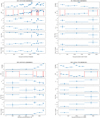 |
Fig. 1. Top panels: adaptively rebinned light curve in the full energy band (0.5–10 keV) for each source. Second panel from the top: corresponding HR. Vertical solid red lines indicate the time intervals during which the Bayesian block analysis identifies significant changes in the HR and that were used for the extraction of the HR-resolved spectra. The best-fit parameters with 1-σ confidence intervals of the spectra analysis are reported in the panels below (the parameter labeling is the same as in Table 2). |
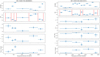 |
Fig. 1. continued. |
In order to determine the best spectral model to be used for the HR resolved spectra, we extracted the average spectrum of each source by integrating over the entire exposure time available in each observation. Being endowed with the best achievable statistics for a specific observation, these total spectra allow us to find the most appropriate description of the source X-ray emission in the XMM-Newton energy band (this is the same technique that we adopted in a number of our previous papers on the SFXTs (see, e.g., Bozzo et al. 2011, 2015, BZ17). The spectral analysis was performed in all cases with Xspec version 12.10.1f (Arnaud 1996 using the W statistic (cstat)) after optimally grouping each source spectrum as described in Kaastra & Bleeker (2016). We excluded from all fits data below 0.55 keV and above 10 keV for the EPIC pn and MOS1, while MOS2 data were discarded also between 0.55 keV and 2 keV because of clear instrumental residuals in this energy band in contrast with those observed in the simultaneous MOS1 and EPIC pn spectra (but see also deviations in Sect. 2.2).
Based on our long-standing expertise on the analysis of SFXTs with XMM-Newton, we first attempted to fit the time-averaged spectra of all sources with a simple absorbed power-law model. This model provided acceptable results only in the cases of IGR J18462−0223 and IGR J16328−4726. In all other cases, the simple absorbed power-law model left evident structures in the residuals from the fits at both the lower and upper energy bounds covered by the EPIC cameras. We were able to significantly improve the fits for almost all of these sources (the only exception being IGR J18483−0311; see later in this section) by adopting a power-law model obscured by two layers of neutral absorption, one completely covering the source (TBabs in Xspec) and the other partially extinguishing it (pcfabs). Abundances were set to Wilm (Wilms et al. 2000) and cross section to the values reported in Verner et al. (1996) for all cases, following the common approach for SFXT sources and HMXBs in general (see, e.g., Walter et al. 2015, and references therein). Cross-calibration uncertainties and data-selection effects induced by the instrument good time intervals were accounted for in all cases by introducing cross-calibration constants in the fits. These all turned out to be close to unity.
For all fits, we first performed a preliminary minimization using the Levenberg-Marquardt algorithm based on the CURFIT routine from Bevington. We then explored the space of each free parameter using a Monte Carlo Markov chain (MCMC) generated by the Goodman-Weare algorithm with 40 walkers, a length of 26 000, and a burning phase length of 6000. We adopted Jeffreys priors for the unabsorbed power-law flux and absorption column densities. The latter were constrained within the limits of 1021 and 1024 cm−2. We used linear priors for the covering fraction and power-law photon index, limited in the intervals 0−1 and −1−6, respectively. From the posterior distributions, we determined the equivalent 1-σ uncertainties on each fit parameter for each source using the 16 and 84% percentiles. To test the statistical goodness of our model, we took 100 parameter realizations from the MCMC and simulated the EPIC spectra with the exposure time and the background count-rate equivalent to the measured ones. We then computed the fit statistics and compared the resulting distribution with the best-fit value. Generally, we found that from 20 to 60% of the simulated spectra were characterized by a C-stat larger than the best-fit C-stat. There are two exceptions to this finding. The first concerns OBSID 0823990901, for which the time-averaged spectrum is noisy at low energy owing to background fluctuations, and the second concerns OBSID 0823990201, whose time-averaged spectrum showed convincing evidence for an additional spectral component below ∼2 keV (see below).
We note that the Bayesian posterior sampling could be sensitive to the particular algorithm used to explore the parameter space, and therefore we also verified that the posteriors determined with the Goodman-Weare algorithm were consistent with the ones determined using the multi-nest method (Feroz et al. 2009) in each average spectrum. For this task, we exploited the BXA interface to Xspec (Buchner et al. 2014). Results were in all cases consistent (within uncertainties), and so in the following we use and report only the results obtained with the Goodman-Weare algorithm.
The results of this analysis are shown in Table 2. For all these sources, the same model was also used to fit the HR-resolved spectra and all results (best-fit spectral parameters vs. time) are shown in Fig. 1. We note that in the case of the source IGR J18462−0223 only the time-averaged spectrum was extracted due to the low statistics of the data and the lack of any significant HR variability.
Summary of the results obtained from the fits to the average spectra from the XMM-Newton observation of each considered source.
The only source for which averaged and HR-resolved spectra could not yet be satisfactorily fit with the partial absorbed model is IGR J18483−0311 (OBSID 0823990201). In the case of this source, the fit with the partial absorbed model left evident residuals at energies ≲1.8 keV. We attempted to improve the fit by changing the partial absorbing component with any other physically motivated component usually adopted for SFXTs (e.g., black body, disk black body, breemstrahlung, additional power-law). None of these attempts resulted in an acceptable fit. We therefore concluded that a further spectral component was needed in addition to those already included in our partially absorbed model. We found that the addition of a component likely emerging from the wind of the supergiant star (see, e.g., Bozzo et al. 2010; Sidoli 2010) and originated from a plasma in ionization equilibrium (APEC model in XSPEC) could remove the most significant structures in the fit residuals (see Fig. 2). We summarize all results obtained from the fit with this model to the IGR J18483−0311 data in Table 3.
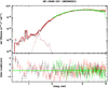 |
Fig. 2. Unfolded spectrum of IGR J18483−0311, together with the best-fit model summarized in Table 3. The residuals from the fit are shown in the lower panel. Data points and lines in black correspond to the EPIC-pn data, while those in red and green represent the MOS1 and MOS2 data, respectively. |
We verified that the parameters of the APEC component could not be constrained in the fits to the HR-resolved spectra of IGR J18483−0311, and therefore we kept in these cases both the APEC temperature and column density fixed to the values measured from the time-averaged spectrum. Only the normalization of the APEC component was left free to vary in the HR-resolved spectra (see Fig. 3 for the best-fit parameters).
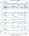 |
Fig. 3. Same as Fig. 1 but in the case of the source IGR J18483−0311, which is the only one requiring the addition of an APEC component to satisfactorily fit its time-averaged spectrum (see text for more details). |
We performed a systematic search for correlations between the best-fit parameters obtained from the HR-resolved spectra of all analyzed sources. In each source, the linear correlation was computed between two fit parameters taking into account uncertainties in both variables and extracting their values from a symmetric Gaussian distribution with standard deviation determined from half the 16–84% posterior interval. We were not able to find any significant correlation, the only exception being the obvious case of the source IGR J16418−4532, where the covering fraction appears to be clearly anti-correlated with the count rate (see Fig. 4). In this case, the Person’s coefficient 1-σ interval in our bootstrapped realization is contained between 0.48 and 0.62, while the slope is −0.14 ± 0.02 at 68% c.l.
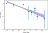 |
Fig. 4. Correlation between the covering fraction and the source count rate in IGR J16418−4532 (OBSID 0823990401). The shaded region indicates the envelope of the correlation curves at 1σ confidence level. |
2.2. Optimization of our standard analysis
We list in this section a few deviations from the description of the general data reduction and analysis provided in the previous section. Although the main analysis steps are the same for all observations, as illustrated below, some data sets required some ad-hoc adjustment of the general procedure to avoid any spurious alteration of the spectral-fit outcomes. This has been a common practice for our previous publications on the subject (see, e.g., BZ17). For OBSID 0823990201, we excluded data after 2019-04-07 at 11:10:56 because a particularly bright solar flare made the data unusable from this time until the end of the planned exposure. No other filtering was required in the remaining part of the observation. For this observations, the somewhat lower absorption than in other cases (see Sect. 3) allowed us to also use MOS2 data in the energy range 0.55−2 keV as no anomalous residuals were found compared to the other EPIC cameras. For OBSID 0823990401, we excluded EPIC-pn data up to 2 keV and MOS1 from 1.2 to 1.5 keV, due to evident background-induced residuals. For OBSID 0823990601, we used for the scientific analysis only data collected from 2018-08-28 at 10:47:44 onward, that is, 16 ks after the nominal start of observation. This was necessary in order to exclude an initial time interval in which the source was too weak to obtain meaningful results. Only a few minor solar flares were observed in the following period, resulting in an almost negligible good time interval filtering. The lower energy bound of EPIC-pn data for the spectral analysis is set to 2 keV because of residuals in the fits not compatible with those of the MOS1, indicating a clear instrumental origin. For the same reason, MOS2 data were excluded below 3 keV. As known from previous publications (Zurita Heras & Chaty 2009), IGR J18450−0435 is located close to a known active galactic nucleus. Therefore, in OBSID 0844100701, we limited the source-extraction region to 640 pixels in imaging mode and to a width of 32 RAWX units for timing mode. In the case of OBSID 0823990901, MOS1 was operated with a closed filter for virtually all available observational time and no useful data could be exploited for the scientific analysis. Due to instrumental residuals, the MOS2 data below 3 keV were ignored.
2.3. Computation of flux upper limits
During OBSID 0823990301 and 0844100101, the targets were not detected by XMM-Newton. To compute the upper limits on their X-ray emission, we searched in the literature for the most common spectral model used to describe the X-ray emission from IGR J11215−5952 and IGR J18410−0535 in an energy band compatible with that of the XMM-Newton EPIC cameras. For IGR J18410−0535, we adopted the absorbed-power-law model used by Bozzo et al. (2011) in the first bin of their light curve. To the best of our knowledge, this is the most accurate description of the source spectrum at low luminosity. For IGR J11215−5952, we adopted the partial covering model for the average spectrum reported in Sidoli et al. (2017, their model 2 in Table 1). We set Gaussian priors to all model parameters except the integrated flux of the power law in the 1–10 keV band, for which we use a Jeffrey’s prior. The Gaussian average is the literature best-fit parameters, while the standard deviation is the average of the upper and lower uncertainties scaled at 68% c.l. We used data for EPICpn only, as it is critical to estimate the background very close to the source and this is better achieved in full window mode. After running the Goodman-Weaver MCMC chain in Xspec, we determined the upper 90% percentile on the normalization as the unabsorbed flux upper limit. The results are reported in Table 1. For the MOS cameras, uncertainties linked to background subtractions far from the source-extraction region prevent a meaningful estimation of the upper limit.
3. Results
The light curves of the different sources displayed in the top panels of Fig. 1 show that our observational program has been successful, as up to several flares are detected in most of the ∼20 ks XMM-Newton pointings. This was expected based on our current knowledge of the SFXTs from literature results and long-term studies carried out especially with Swift/XRT. The only exceptions are the sources IGR J11215−5952 and IGR J18410−0535, which were not detected during the XMM-Newton observation, as well as the source IGR J18462−0223, which was caught in a low activity state. We comment below individually on the results obtained for each source included in the present study.
IGR J18483−0311: Our XMM-Newton observation found the source in a remarkably active state and a total of at least six flares were recorded in less than 30 ks. Some of these flares achieve a count rate as high as ∼25 cts s−1 in the EPIC-pn camera (see Fig. 3). Although the observed flares are bright, the variations of the HR are relatively limited (less than a factor of two). Looking at the relevant plot in Fig. 3, we note that the lowest HR values are recorded in between flares around 10 ks, 12 ks, 17 ks, and 24 ks from the beginning of the observation. The analysis of the HR-resolved spectra revealed hints of a lower covering fraction during the low-HR time intervals (especially for the interval around 24 ks) and a correspondingly increased absorption column density. There seems to be some evidence for a larger covering fraction during the rises and peaks of the flares, although our sample size is not sufficiently large to obtain any statistically significant results (throughout the paper we refer to rises and decays of the SFXT flares following the same definition and approach used in our previous paper BZ17). The normalization of the APEC component was in general poorly constrained and we could not find indications of any significant variability during the selected time intervals for the spectral analysis. However, it should be noted that including this component in all fits avoided any bias during the comparison of the results obtained from different time intervals.
IGR J16418−4532: Among the observations presented in this paper, OBSID 0823990401 is certainly the most interesting. Looking at the relevant plot in Fig. 1, we can see that the source underwent at least five distinct flares and displayed a progressively decreasing HR which varied by a factor of approximately seven between the beginning and end of the observation. Apart from the overall progressive decrease, the recorded HR shows significant increases at the flare rises and abrupt decreases toward the flare peaks. The results of our spectral analysis reported in Fig. 1 confirm that the progressive change in the HR is due to a variation of the column density. This analysis shows that the increases of the HR during the rises to the flares are also associated with increases in the absorption column density, while the drops of the HR during the peaks of the flares are associated with both a decrease in the absorption column density and in the covering fraction. This conclusion is further confirmed by the detection of a significant anti-correlation between the source count rate and the covering fraction displayed in Fig. 4 and introduced earlier in Sect. 2.1.
We note that these variations cannot be related to the pulsations from the source as the latter occur recurrently on a much shorter timescale (∼1210 s; see, e.g., Drave et al. 2013, and references therein). To search for pulsations in our data set, we performed an epoch folding search (Leahy 1987) on the combined 0.5–10 keV light curve of the source with bins of 10 s. We explored frequencies from 0.5 to 3.3 mHz with no weighting using 16 phase bins. The lower limit is chosen to exclude the secular trend from the periodogram red noise and the upper limit is determined from the light-curve binning. To subtract the red noise, we fit a power law to the frequency dependency of the χ2 and found a slope of 0.99 ± 0.03 with normalization at 1 Hz of 3.1 ± 0.5 × 10⁻³. We subtract this function and add the expectation value of a χ2 distribution with 15 degrees of freedom and obtain the curve of Fig. 5. The most prominent peak is at a frequency of 0.827 ± 0.003 mHz, corresponding to a period of 1208 ± 4 s; two other peaks are present at twice and three times the base frequency. We consider the peak at 1.25 mHz as spurious. Following D’Aì et al. (2011), we determine the period uncertainty as Pmax/2NphΔt, where Pmax is the peak frequency, ΔT the observation duration, and Nph the number of trial phase bins. To asses the significance of the peak, we compute an exponential fit to the histogram of de-redenned χ2 between the values 20 and 50 using an exponential function (K exp(−bχ2)). We find K = 230 ± 30 and  at 68% c.l. We then compute the 90% quantile of the integrals of the normalized exponential fitting function above the χ2 value of the peak. Converting this probability into standard deviations of a normal distribution, we find that the main peak has an equivalent significance of 3.7σ. If we compute the combined probability that also the harmonics are present, we reach a robust detection of the pulsation at 5σ. Our detection of the spin period in these observations is in line with previous findings by Sidoli et al. (2012) and Drave et al. (2013) and does not yield any measurable spin evolution.
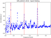 |
Fig. 5. Periodogram of IGR J16418−4532 (OBSID 0823990401) obtained with epoch folding using 16 phase bins. Red noise has been modeled and subtracted. The red vertical dashed lines correspond to the pulse frequency of 0.827 mHz and its two harmonics. |
AX J1949.8+2534: this source was caught by XMM-Newton in a relatively faint state, but we recorded an overall variation in the HR by a factor of ∼2.5 across the observation. The results of the HR-resolved spectral analysis in Fig. 1 suggest a similar situation to that reported for the previous source, with an overall decrease of the absorption column density during the observation, although these variations are marginally significant. There is evidence of a short, faint flare about 13 ks after the beginning of the observation but the event was too brief (about 1 ks) and was too faint to carry out any meaningful, more detailed investigation.
IGR J16479−4514: This source displayed a remarkable increasing HR, reaching a value about ten times higher from the beginning up to the first 12 ks of the observation and undergoing an abrupt decrease by a factor of approximately two at the very end of the observation (the last ks; see Fig. 1). The progressive increase in the HR together with the corresponding increase in the source count rate strongly resemblers what is usually observed during the egress from an X-ray eclipse. IGR J16479−4514 is known to display X-ray eclipses (see, e.g., Bozzo et al. 2009), and if we consider the most recently published ephemeris of the source (Coley et al. 2015), it is possible to show that the XMM-Newton observation studied in this paper is compatible with being the egress from an eclipse. The increase in the source count-rate across the XMM-Newton observation is therefore likely associated with the source ramping up to its usual emission state and it is not a flare. The sudden drop in the HR at the very end of the observation remains puzzling. Results of the HR-resolved spectral analysis do not show a clear trend and it is likely that the progressive increase in the HR is the combined effect of slight variations in several parameters (absorption column density, covering fraction, power-law photon index). There is some evidence that a decrease in absorption column density and an increase in the covering fraction may explain the abrupt decrease of the HR in the last thousand seconds of this observation.
SAX J1818.6−1703: This source underwent two relatively faint flares during the XMM-Newton observation (Fig. 1). Although the data signal to noise ratio is far too low to perform a detailed study of the HR variations within the rises and decays of the two flares, our HR-resolved spectral analysis (Fig. 1) revealed a progressive increase in the absorption column density during the entire observation, accompanied by a softening of the power law and a marginally significant decrease of the covering fraction. Although the source ephemeris has been reported in the literature (Bird et al. 2010), we were unable to determine the orbital phase of the present XMM-Newton observation. This is due to the relatively large uncertainty associated with the orbital period in the available parameters and the extrapolation of the orbital phase up to 2019.
IGR J16328−4726: This source underwent two flares during the observation and displayed a relatively limited but interesting variation of the HR (see Fig. 1). The HR is observed to increase toward the peak of the flares and decrease between them. Our HR-resolved spectral analysis revealed that the increase is the result of two opposite effects. On the one hand, the absorption column density rises at the onset of the flare and decreases toward the peak. On the other hand, there is a substantial hardening of the power-law photon index from the onset to the peak of the flare that compensates the variation of the absorption column density and contributes to making the overall source spectral emission harder at the peaks of both recorded flares. The emission during the quiescent time interval between the two flares is characterized by a low HR which results uniquely from the low absorption column density (the lowest measured during the entire observation) as the power-law photon index is the hardest measured across the ∼25 ks spanned in the OBSID 0823990901.
IGR J18450−0435: This source underwent three faint flares during the ∼20 ks XMM-Newton observation. Although its flux is similar to that of the source SAX J1818.6−1703, the overall variation of the HR was slightly less pronounced (Fig. 1) and our HR-resolved spectral analysis could not identify any significant spectral change (although all measured values of the spectral parameters are endowed with fairly large error bars; see Fig. 1).
4. Discussion and conclusions
This paper reports the results obtained from the first ten observations of our ongoing monitoring program of the SFXTs with XMM-Newton and serves as a demonstration that our program, although it began only recently, is successfully delivering the expected outcomes. The program is carrying out observations in the direction of all known SFXTs, each of roughly 20 ks in duration, in order to populate the database of flares observed from these sources with the only X-ray facility that is endowed at present with sufficient sensitivity and spectral resolution to detect fast spectral variations during these events. As discussed in the literature, such studies might ultimately help us to understand the mechanism(s) driving the peculiar behavior of the SFXTs in X-rays (see also Sect. 1). So far, most of the already performed 20 ks pointings caught from one to six flares from the targeted SFXTs.
The richest dataset acquired so far, and certainly the most intriguing, is that for the SFXT IGR J16418−4532. This source displayed a progressive decrease in absorption column density along the entire XMM-Newton observation in addition to significant swings of the same spectral parameter during the rise and decay from the flares3. This behavior is remarkably similar to that observed in the case of the SFXT IGR J17354−3255 during the XMM-Newton OBSID 0693900201 (see Fig. 9 in BZ17). Following our previous interpretation of the event from IGR J17354−3255, we also suggest that in the case of IGR J16418−4532, XMM-Newton might have observed a relatively rare case in which a large massive clump passed in front of the neutron star along the line of sight to the observer. Such an event causes substantial obfuscation of the X-ray source due to the increased local absorption column density, and the flares that are observed during the pointing are likely triggered by some part of this possibly structured clump onto the NS. Interestingly, the reported increases in the absorption column density during the rises of flares and the abrupt decreases close to the peaks are similar to what has been observed in the past in several SFXTs (BZ17). These decreases were interpreted as being due to the approach of a clump (or some structures within it) to the neutron star (during the rises from the flare) and the photoionization of the clump material shortly after the flare reached a sufficiently high luminosity (close to the peak). The significant anti-correlation between the count rate and the absorption covering fraction is a further indication that increasing radiation tends to clear up wind clumps around the neutron star. These trends in the spectral variability support the idea that clumps play a major role in triggering the flares and/or outbursts from SFXTs. However, as mentioned in previous studies, it cannot be excluded that additional mechanisms are at work to inhibit accretion in SFXTs for most of the time and permit accretion only when the increase in the local mass accretion rate caused by the clump is hampering their effectiveness in controlling the accretion flow (see, e.g., the discussion in Bozzo et al. 2015, and references therein).
In the past, IGR J16418−4532 has also shown other episodes of intriguing X-ray activity. During another XMM-Newton observation, Drave et al. (2013) reported a large temporary increase in the local absorption column density that lasted about 1 ks and occurred slightly before the rise of a flare. This occurrence was also interpreted in terms of a clump approaching the NS and then being accreted onto the compact object (giving rise to the subsequent X-ray flares). In 2011, a peculiar episode of unusual low-variability emission was observed with XMM-Newton and ascribed to the possible switch from the usual wind-accretion regime to a Roche-Lobe overflow regime, during which an accretion disk is suspected to form around the NS (Sidoli et al. 2012). This conclusion remained speculative, given the lack of direct evidence of the presence of an accretion disk, as well as the lack of other similar events during later observations of the source. Although the dynamic range of the X-ray luminosity displayed by IGR J16418−4532 is somewhat on the low side compared to most of the SFXTs (see also the discussion in Bozzo et al. 2015), the observational findings on this source make it one of the most promising candidates to search for spectral variability during and in between flares.
A number of other sources reported in this paper showed some similarity in their spectral variability during flares with IGR J16418−4532, especially for what concerns the changes in the absorption column density. Of particular interest for the goal of our analysis is the detection of enhancements in the absorption column density just before or during the rise of a flare, as well as the decrease in the nH at the peak of the flares. As summarized in Sect. 1 and briefly mentioned earlier in this section, similar indications support the idea that clumps are key players in driving the variability of SFXTs. In Sect. 3, we show that evidence for a similar behavior could be obtained for IGR J16328−4726 and, albeit with greater uncertainty due to the low sample size, in the source AX J1949.8+2534. IGR J16479−4514 showed evidence of decreasing absorption column density close to the peak of a possible flare, although this result has to be taken with caution because XMM-Newton most likely caught the source while emerging from an X-ray eclipse.
For the remaining sources, the interpretation is less clear. IGR J18483−0311 displayed several bright flares but despite the highest count rate achieved compared to all other sources presented here, the overall variation of HR remained relatively low. We were not able to reveal the expected rises of the nH close to the onset of the flares, or the drops around their peaks. We found evidence of a larger covering fraction during the most intense X-ray luminosity time intervals and lower values of the same parameter during the times between the flares. In the context of a clumpy wind interpretation, we could argue that during this specific XMM-Newton pointing the source was located in a particularly dense region of the wind and flares were triggered by just modest variations of the local mass accretion rate likely overwhelming the effect of the mechanisms usually inhibiting accretion. The higher covering fraction during the flare might indeed be connected to the slightly larger amount of accreting material from the stellar wind approaching the NS. A similar scenario could be applicable in the case of SAX J1818.6−1703, which showed tentative evidence of a decrease in the covering fraction during the lowest emission time interval toward the end of the XMM-Newton observation. The soft APEC component revealed in the spectrum of IGR J18483−0311 could not be studied in great detail, because few counts are recorded below ∼2 keV (especially its variation as a function of time and/or HR). However, its detection is already quite interesting because it likely indicates the presence of a strong stellar wind, as suggested in the case of a similar soft spectral component revealed in the X-ray emission of the SFXT IGR J08408−4503 (Bozzo et al. 2010; Sidoli 2010). Should shocks be present in supergiant star winds, as predicted by one-dimension numerical simulations (Feldmeier 1995; Feldmeier et al. 1997), at least part of the flares could be due to drops of the wind speed and consequent increases of the accretion radius. These flares would not be necessarily associated to column density enhancements.
In the cases of IGR J16479−4514 and IGR J18450−0435, we were not able to investigate the HR variations in detail because of the complication of the egress from the eclipse and the low signal to noise, respectively. Previous publications in the literature have shown that these sources can display extreme variability (see, e.g., BZ17, Sidoli et al. 2006, 2017; Zurita Heras & Chaty 2009, and references therein), and therefore additional observations with XMM-Newton in the future might help us to catch bright flares and achieve a better understanding of the physical conditions in their accretion environments.
Two sources in our sample were not detected during the corresponding XMM-Newton observation. In the case of IGR J11215−5952, we determined a 90% c.l. upper limit of 6 × 10⁻¹⁵ erg cm−2 s−1 on its 1−10 keV unabsorbed X-ray emission, corresponding to a luminosity of 4 × 1031 erg s−1 (assuming a distance of 7 kpc; see Sidoli et al. 2017, and references therein). To the best of our knowledge, this is the lowest flux ever recorded from this source (see also Sidoli et al. 2020, for recent nondetections). This low luminosity, if confirmed, would not be surprising, as IGR J11215−5952 is known to have a long and eccentric orbit which would naturally cause the mass accretion rate to drop dramatically when the NS is far away from periastron. As the orbital period of the source is ∼165 days and the last accurately observed outburst occurred on 2016 February 14, we conclude that the XMM-Newton observation took place about 60 days after the closer expected outburst, likely in a region of the orbit where the mass accretion rate is too low to give rise to detectable X-ray emission. Although we only have one deep upper limit so far, the availability of further high-sensitivity observations with XMM-Newton along the orbit of IGR J11215−5952 might help us to make a full comparison with the NS Be X-ray binaries which are endowed with similarly high eccentricity and elongated orbits but are often also detected in X-rays (including pulsations) during time intervals away from periastron (see Doroshenko et al. 2014, and references therein). Due to its peculiar orbital configuration and the uniqueness of its periodic outbursts among the SFXT sources, it was already claimed in previous papers that IGR J11215−5952 could be the missing link between SFXTs and the longer known class of Be X-ray binaries (Liu et al. 2011).
The estimated upper limit on the X-ray emission from IGR J18410−0535 measured during the XMM-Newton observation 0844100101 provided, to the best of our knowledge, again the lowest luminosity value for this object (see Sidoli et al. 2008; Bozzo et al. 2011, and references therein). As our upper limit is a factor of approximately ten deeper than previously reported values, this result increases the dynamic range displayed by IGR J18410−0535 up to ∼5 × 10⁴. This is still well within the dynamic ranges displayed by the SFXTs, with a maximum of ∼106 being achieved by IGR J17544−2619 (Romano et al. 2015).
As evidenced by the above summary, the monitoring program of the SFXTs that we are pursuing with XMM-Newton is already providing intriguing and useful results, in accordance with expectations. Further XMM-Newton observations of a similar duration to those reported here are currently ongoing for a number of other confirmed SFXT sources. When a large number of flares per source have been observed (≳25), it will be possible to perform more statistically signficant analyses on the properties of the fast spectral variability during these events across the entire SFXT class, as suggested and initiated by BZ17. This will be a powerful tool to significantly improve our understanding of the mechanisms triggering the peculiar X-ray variability of SFXTs, possibly going quantitatively beyond the simplistic assumption that most of the variability is related to stellar wind clumps and providing reliable estimates of the physical properties of these structures in cases where they are being accreted by the NS and cases where they are simply passing along our line of sight to the compact object.
So far, the presence of a NS instead of a black hole in most of the SFXTs is based on the spectral energy distribution in the X-ray domain that in all cases is remarkably similar to that of X-ray pulsars. Pulsations have been detected only in two out of the roughly ten known SFXTs.
We note that our XMM-Newton observation did not occur during the eclipse of the source as the time of the observation is incompatible with the expected times according to the ephemeris reported by Coley et al. (2015) also when all uncertainties are taken into account.
Acknowledgments
We thank the anonymous referee for their useful comments which helped us improving the paper. This research made use of Astropy (http://www.astropy.org), a community-developed core Python package for Astronomy (Astropy Collaboration 2018). For plotting, we exploited the Matplotlib python package (Hunter 2007). To consistently perform the analysis, we developed a python wrapper to particular SAS functions, which is publicly available: pyxmmsas.
References
- Arnaud, K. A. 1996, in Astronomical Data Analysis Software and Systems V, eds. G. H. Jacoby, & J. Barnes, ASP Conf. Ser., 101, 17 [Google Scholar]
- Astropy Collaboration (Price-Whelan, A. M., et al.) 2018, AJ, 156, 123 [Google Scholar]
- Bird, A. J., Bazzano, A., Bassani, L., et al. 2010, ApJS, 186, 1 [NASA ADS] [CrossRef] [Google Scholar]
- Bozzo, E., Falanga, M., & Stella, L. 2008, ApJ, 683, 1031 [NASA ADS] [CrossRef] [Google Scholar]
- Bozzo, E., Stella, L., Israel, G., Falanga, M., & Campana, S. 2009, in AIP Conf. Ser., eds. J. Rodriguez, & P. Ferrando, 1126, 319 [CrossRef] [Google Scholar]
- Bozzo, E., Stella, L., Ferrigno, C., et al. 2010, A&A, 519, A6 [NASA ADS] [CrossRef] [EDP Sciences] [Google Scholar]
- Bozzo, E., Giunta, A., Cusumano, G., et al. 2011, A&A, 531, A130 [NASA ADS] [CrossRef] [EDP Sciences] [Google Scholar]
- Bozzo, E., Romano, P., Ducci, L., Bernardini, F., & Falanga, M. 2015, Adv. Space Res., 55, 1255 [NASA ADS] [CrossRef] [Google Scholar]
- Bozzo, E., Bernardini, F., Ferrigno, C., et al. 2017, A&A, 608, A128 [NASA ADS] [CrossRef] [EDP Sciences] [Google Scholar]
- Buchner, J., Georgakakis, A., Nandra, K., et al. 2014, A&A, 564, A125 [NASA ADS] [CrossRef] [EDP Sciences] [Google Scholar]
- Coley, J. B., Corbet, R. H. D., & Krimm, H. A. 2015, ApJ, 808, 140 [NASA ADS] [CrossRef] [Google Scholar]
- D’Aì, A., La Parola, V., Cusumano, G., et al. 2011, A&A, 529, A30 [NASA ADS] [CrossRef] [EDP Sciences] [Google Scholar]
- Doroshenko, V., Santangelo, A., Doroshenko, R., et al. 2014, A&A, 561, A96 [NASA ADS] [CrossRef] [EDP Sciences] [Google Scholar]
- Drave, S. P., Bird, A. J., Sidoli, L., et al. 2013, MNRAS, 433, 528 [NASA ADS] [CrossRef] [Google Scholar]
- El Mellah, I., & Casse, F. 2017, MNRAS, 467, 2585 [NASA ADS] [Google Scholar]
- El Mellah, I., Sundqvist, J. O., & Keppens, R. 2018, MNRAS, 475, 3240 [NASA ADS] [CrossRef] [Google Scholar]
- Feldmeier, A. 1995, A&A, 299, 523 [NASA ADS] [Google Scholar]
- Feldmeier, A., Puls, J., & Pauldrach, A. W. A. 1997, A&A, 322, 878 [NASA ADS] [Google Scholar]
- Feroz, F., Hobson, M. P., & Bridges, M. 2009, MNRAS, 398, 1601 [NASA ADS] [CrossRef] [Google Scholar]
- Hainich, R., Oskinova, L. M., Torrejón, J. M., et al. 2020, A&A, 634, A49 [Google Scholar]
- Hunter, J. D. 2007, Comput. Sci. Eng., 9, 90 [NASA ADS] [CrossRef] [Google Scholar]
- in’t Zand, J. J. M. 2005, A&A, 441, L1 [NASA ADS] [CrossRef] [EDP Sciences] [Google Scholar]
- Jansen, F., Lumb, D., Altieri, B., et al. 2001, A&A, 365, L1 [NASA ADS] [CrossRef] [EDP Sciences] [Google Scholar]
- Kaastra, J. S., & Bleeker, J. A. M. 2016, A&A, 587, A151 [NASA ADS] [CrossRef] [EDP Sciences] [Google Scholar]
- Leahy, D. A. 1987, A&A, 180, 275 [NASA ADS] [Google Scholar]
- Liu, Q. Z., Chaty, S., & Yan, J. Z. 2011, MNRAS, 415, 3349 [NASA ADS] [CrossRef] [Google Scholar]
- Lutovinov, A. A., Revnivtsev, M. G., Tsygankov, S. S., & Krivonos, R. A. 2013, MNRAS, 431, 327 [NASA ADS] [CrossRef] [Google Scholar]
- Martínez-Núñez, S., Kretschmar, P., Bozzo, E., et al. 2017, Space Sci. Rev., 212, 59 [NASA ADS] [CrossRef] [Google Scholar]
- Negueruela, I. 2010, in High Energy Phenomena in Massive Stars, eds. J. Martí, P. L. Luque-Escamilla, & J. A. Combi, ASP Conf. Ser., 422, 57 [Google Scholar]
- Pradhan, P., Bozzo, E., & Paul, B. 2018, A&A, 610, A50 [NASA ADS] [CrossRef] [EDP Sciences] [Google Scholar]
- Rampy, R. A., Smith, D. M., & Negueruela, I. 2009, ApJ, 707, 243 [NASA ADS] [CrossRef] [Google Scholar]
- Romano, P., Krimm, H. A., Palmer, D. M., et al. 2014a, A&A, 562, A2 [NASA ADS] [CrossRef] [EDP Sciences] [Google Scholar]
- Romano, P., Ducci, L., Mangano, V., et al. 2014b, A&A, 568, A55 [NASA ADS] [CrossRef] [EDP Sciences] [Google Scholar]
- Romano, P., Bozzo, E., Mangano, V., et al. 2015, A&A, 576, L4 [NASA ADS] [CrossRef] [EDP Sciences] [Google Scholar]
- Scargle, J. D., Norris, J. P., Jackson, B., & Chiang, J. 2013, ApJ, 764, 167 [NASA ADS] [CrossRef] [Google Scholar]
- Shakura, N., Postnov, K., Kochetkova, A., & Hjalmarsdotter, L. 2012, MNRAS, 420, 216 [NASA ADS] [CrossRef] [Google Scholar]
- Shakura, N., Postnov, K., Sidoli, L., & Paizis, A. 2014, MNRAS, 442, 2325 [NASA ADS] [CrossRef] [Google Scholar]
- Sidoli, L. 2010, AIP Conf. Proc., 1314, 271 [NASA ADS] [CrossRef] [Google Scholar]
- Sidoli, L., Paizis, A., & Mereghetti, S. 2006, A&A, 450, L9 [NASA ADS] [CrossRef] [EDP Sciences] [Google Scholar]
- Sidoli, L., Romano, P., Mangano, V., et al. 2008, ApJ, 687, 1230 [NASA ADS] [CrossRef] [Google Scholar]
- Sidoli, L., Mereghetti, S., Sguera, V., & Pizzolato, F. 2012, MNRAS, 420, 554 [NASA ADS] [CrossRef] [Google Scholar]
- Sidoli, L., Tiengo, A., Paizis, A., et al. 2017, ApJ, 838, 133 [NASA ADS] [CrossRef] [Google Scholar]
- Sidoli, L., Postnov, K. A., Belfiore, A., et al. 2019, MNRAS, 487, 420 [CrossRef] [Google Scholar]
- Sidoli, L., Postnov, K., Tiengo, A., et al. 2020, A&A, 638, A71 [CrossRef] [EDP Sciences] [Google Scholar]
- Strüder, L., Briel, U., Dennerl, K., et al. 2001, A&A, 365, L18 [NASA ADS] [CrossRef] [EDP Sciences] [Google Scholar]
- Turner, M. J. L., Abbey, A., Arnaud, M., et al. 2001, A&A, 365, L27 [NASA ADS] [CrossRef] [EDP Sciences] [Google Scholar]
- Verner, D. A., Ferland, G. J., Korista, K. T., & Yakovlev, D. G. 1996, ApJ, 465, 487 [NASA ADS] [CrossRef] [Google Scholar]
- Walter, R., & Zurita Heras, J. 2007, A&A, 476, 335 [Google Scholar]
- Walter, R., Lutovinov, A. A., Bozzo, E., & Tsygankov, S. S. 2015, A&ARv, 23, 2 [NASA ADS] [CrossRef] [Google Scholar]
- Wilms, J., Allen, A., & McCray, R. 2000, ApJ, 542, 914 [NASA ADS] [CrossRef] [Google Scholar]
- Zurita Heras, J. A., & Chaty, S. 2009, A&A, 493, L1 [NASA ADS] [CrossRef] [EDP Sciences] [Google Scholar]
All Tables
Summary of the results obtained from the fits to the average spectra from the XMM-Newton observation of each considered source.
All Figures
|
Fig. 1. Top panels: adaptively rebinned light curve in the full energy band (0.5–10 keV) for each source. Second panel from the top: corresponding HR. Vertical solid red lines indicate the time intervals during which the Bayesian block analysis identifies significant changes in the HR and that were used for the extraction of the HR-resolved spectra. The best-fit parameters with 1-σ confidence intervals of the spectra analysis are reported in the panels below (the parameter labeling is the same as in Table 2). |
| In the text | |
|
Fig. 1. continued. |
| In the text | |
|
Fig. 2. Unfolded spectrum of IGR J18483−0311, together with the best-fit model summarized in Table 3. The residuals from the fit are shown in the lower panel. Data points and lines in black correspond to the EPIC-pn data, while those in red and green represent the MOS1 and MOS2 data, respectively. |
| In the text | |
|
Fig. 3. Same as Fig. 1 but in the case of the source IGR J18483−0311, which is the only one requiring the addition of an APEC component to satisfactorily fit its time-averaged spectrum (see text for more details). |
| In the text | |
|
Fig. 4. Correlation between the covering fraction and the source count rate in IGR J16418−4532 (OBSID 0823990401). The shaded region indicates the envelope of the correlation curves at 1σ confidence level. |
| In the text | |
|
Fig. 5. Periodogram of IGR J16418−4532 (OBSID 0823990401) obtained with epoch folding using 16 phase bins. Red noise has been modeled and subtracted. The red vertical dashed lines correspond to the pulse frequency of 0.827 mHz and its two harmonics. |
| In the text | |
Current usage metrics show cumulative count of Article Views (full-text article views including HTML views, PDF and ePub downloads, according to the available data) and Abstracts Views on Vision4Press platform.
Data correspond to usage on the plateform after 2015. The current usage metrics is available 48-96 hours after online publication and is updated daily on week days.
Initial download of the metrics may take a while.