| Issue |
A&A
Volume 641, September 2020
|
|
|---|---|---|
| Article Number | A35 | |
| Number of page(s) | 37 | |
| Section | Interstellar and circumstellar matter | |
| DOI | https://doi.org/10.1051/0004-6361/202037511 | |
| Published online | 04 September 2020 | |
Dark dust and single-cloud sightlines in the ISM
1
European Southern Observatory,
Karl-Schwarzschild-Str. 2,
85748
Garching,
Germany
e-mail: This email address is being protected from spambots. You need JavaScript enabled to view it.
2
Rzeszów University,
al. T. Rejtana 16c,
35-959
Rzeszów, Poland
3
European Southern Observatory,
Alonso de Cordova 3107,
Vitacura,
Santiago, Chile
4
Instituto de Astronomia, Universidad Catolica del Norte,
Av. Angamos 0610,
Antofagasta, Chile
5
Pulkovo Observatory,
Pulkovskoe Shosse 65,
Saint-Petersburg
196140,
Russia
6
Armagh Observatory and Planetarium,
College Hill,
Armagh
BT61 9DG, UK
Received:
15
January
2020
Accepted:
15
June
2020
Abstract
The precise characteristics of clouds and the nature of dust in the diffuse interstellar medium can only be extracted by inspecting the rare cases of single-cloud sightlines. In our nomenclature such objects are identified by interstellar lines, such as K I, that show at a resolving power of λ∕Δλ ~ 75 000 one dominating Doppler component that accounts for more than half of the observed column density. We searched for such sightlines using high-resolution spectroscopy towards reddened OB stars for which far-UV extinction curves are known. We compiled a sample of 186 spectra, 100 of which were obtained specifically for this project with UVES. In our sample we identified 65 single-cloud sightlines, about half of which were previously unknown. We used the CH/CH+ line ratio of our targets to establish whether the sightlines are dominated by warm or cold clouds. We found that CN is detected in all cold (CH/CH+ > 1) clouds, but is frequently absent in warm clouds. We inspected the WISE (3−22 μm) observed emission morphology around our sightlines and excluded a circumstellar nature for the observed dust extinction. We found that most sightlines are dominated by cold clouds that are located far away from the heating source. For 132 stars, we derived the spectral type and the associated spectral type-luminosity distance. We also applied the interstellar Ca II distance scale, and compared these two distance estimates with Gaia parallaxes. These distance estimates scatter by ~40%. By comparing spectral type-luminosity distances with those of Gaia, we detected a hidden dust component that amounts to a few mag of extinction for eight sightlines. This dark dust is populated by ≳ 1 μm large grains and predominately appears in the field of the cold interstellar medium.
Key words: ISM: clouds / dust, extinction / ISM: lines and bands / stars: early-type
© ESO 2020
1 Introduction
The main physical and chemical characteristics of the interstellar medium (ISM) are obtained by studying six aspects. (a) Interstellar extinction (reddening), which is caused by solid particles of submicron size (Trumpler 1930). (b) Interstellar polarisation (Hong & Greenberg 1980), which is caused by non-spherical dust particles when they are oriented by the magnetic field, for instance. (c) Spectral lines of interstellar atomic gas; see the UV survey by Field (1974), for example, who proved that heavy elements in the ISM are strongly depleted in comparison to their abundances in stellar atmospheres. That is, they are hidden in dust grains. (d) Rotational emission features that have been detected for many (~200) complex molecules with a dipole momentum. (e) Bands of simple molecules or radicals, such as •CH, CH+, •OH, OH+, •SH, •NH, •CN, C2, C3. (f) Diffuse interstellar bands (DIBs) that were discovered by Heger (1922). A census of interstellar and circumstellar diatomics and molecules is given by McGuire (2018). Currently, the list of known DIBs exceeds 550 entries (Fan et al. 2019), and most of them are very shallow. Finally, (g) cosmic rays, which ionise parts of the ISM. Interstellar absorption spectra differ from cloud to cloud, and large variations in the dust properties are observed, e.g. Krełowski et al. (1992, 2019a), Fitzpatrick & Massa (2007), Chini & Kruegel (1983). These differences show that all components mentioned above are interdependent, that is, variations in extinction and/or polarisation curves are accompanied with ratios of various strengths of atomic and/or molecular features.
Individual Doppler components can be resolved into interstellar atomic and/or molecular lines by means of high-resolution spectroscopy, while extinction and continuum polarisation are necessarily averaged along any sightline. Profiles of interstellar features observed at extremely high resolving power of λ∕Δλ ~ 106 with the Ultra-High Resolution Facility (UHRF, Diego et al. 1995) or the McDonald (Tull et al. 1995) instruments reveal multiple Doppler components, e.g. Crane et al. (1995), Barlow et al. (1995), Price et al. (2000), Crawford (2002), Welty & Hobbs (2001), Welty et al. (2003). Strictly speaking, only very few and nearby sightlines can be considered genuine single-cloud sightlines that do not display fine structures in the Doppler profiles of interstellar lines. Clouds are not static entities, however. Dynamically, they may be colliding, merging, or be disrupted. Velocity shears, shells, bubbles, and filamentary structures are observed. Cloud structures are impacted by cosmic rays that change the ionisation structures of the atoms and molecules. Magneto-hydrodynamical waves generate small-scale cloud structures (Falle & Hartquist 2002). Shocks propagating through the ISM can ablate or destroy the clouds (Klein et al. 1994). In some clouds, self-gravitation is at work and forms cloudlets (Wada 2008), which are observed as time-variable interstellar absorption lines, e.g. Falgarone et al. (1991), Lauroesch et al. (2000), Price et al. (2000), Welty & Fitzpatrick (2001), Crawford (2002). Fractal cloud structures (Elmegreen 2002) arise from typically subsonic (≲ 0.7 km s−1) turbulent motions, e.g. Barlow et al. (1995), Welty & Hobbs (2001).
Our project is tailored to study global dust characteristics in clouds, and we do not consider local small-scale variations in the detailed cloud morphology. We assume that a cloud has approximately similar physical dust parameters in grain material, abundance, and sizes, and that grain alignment might be triggered by the global magnetic field structure. In contrast, these dust parameters are assumed to vary on a large scale when clouds are well separated by several 10s or 100s of pc. We use the term single-cloud sightline when the observed interstellar line profiles show one dominant Doppler component in high-resolution spectra at a resolving power of λ∕Δλ ~ 75, 000 (full width at half maximum, FWHM ~ 4 km s−1) that accounts for more than half of the observed column density. Of course some of those single-cloud sightlines may include two or more fine-structure components with slightly different radial velocities (Welty 2014). In fact many such objects are nearby and so the Doppler components must be very close to each other. This proximity is followed by similar spatial motions of the intervening clouds which leads to similar radial velocities. Sightlines with several clouds that are close to each other show similar extinction properties as observed towards associations such as Sco OB2 and Per OB2 (Fitzpatrick & Massa 2007). Therefore, the same properties of the dust and presumably that of the global magnetic field can be assumed. Hence, we apply a less strict nomenclature of single-cloud sightlines as compared to the terminology used by Welty et al. (2003).
Siebenmorgen et al. (2018) have demonstrated that when sightlines are observed that intersect different components (which likely do not resembling each other), the pristine nature of the extinction and polarisation curve of each individual cloud cannot be recovered. The possibility of investigating the relation between the physical parameters of the dust is lost, as are the observational characteristics of the extinction and polarisation. The only way to investigate these relations is to inspect sightlines that are dominated by single clouds. The Large Interstellar Polarisation Survey (LIPS, Bagnulo et al. 2017) allowed us to simultaneously fit the extinction and polarisation curves of 59 sightlines. Siebenmorgen et al. (2018) applied a dust model composed of silicate and carbon grains, finding that large (>6 nm) spheroidal silicate particles, which are of prolate shape, account for the observed polarisation curves. For 32 sightlines we complemented the LIPS data set with UVES archive high-resolution spectra. This enabled to extract a small number of 8 single-cloud-dominated sightlines. This study confirmed several correlations between the observed extinction and polarisation characteristics and the physical parameters of the dust, and several previously unknown correlations were found that are significant in single-cloud sightlines alone. This demonstrates the validity of our approach. It was observed that interstellar polarisation from multiple clouds is depolarised and therefore lower than that from single-cloud sightlines, and large variations in the dust characteristics from cloud to cloud is detected. However, when a number of clouds are averaged, a similar mean of the dust parameters is retrieved that represents what is called the Milky Way mean extinction curve; this is an ill-defined average.
In this paper we present a high-resolution spectroscopic search for such single-cloud sightlines at a distance of a few kiloparsec in the solar neighbourhood for which the far-UV extinction curve is known.
2 Observations
Our target selection is aimed at identifying a sample of single-cloud sightlines that are suited for detailed studies of variations in dust properties in the diffuse ISM. For these single-cloud sightlines we require the wavelength dependence of the extinction and polarisation. Therefore we started by considering all 544 sightlines for which the far-UV extinction curves between 0.33 and 0.09 μm were derived from the International Ultraviolet Explorer (IUE, Fitzpatrick & Massa 2007), Valencic et al. (2004) and/or the Far Ultraviolet Spectroscopic Explorer (FUSE, Gordon et al. 2009) satellite data. For these stars we performed an extensive search of available optical high-resolution spectra (λ∕Δλ≳40 000), which enables studying the interstellar line profiles. We found archive spectra for 86 sightlines and conducted new observations for 100 sightlines with the UVES spectrometer, e.g. Dekker et al. (2000) and Smoker et al. (2009).
There are 136 sightlines that have high-resolution spectra with a broad wavelength coverage that is appropriate for a detailed analysis. They are catalogued in Table 1, where we specify (1) the identification number (ID) used in this paper, the target name for which we favour (2) the HD identifier, and if it is different, provide the (3) main name as used in SIMBAD, (4) the V -band magnitude, (5) the reddening E(B − V), (6) the extinction AV, (7) the total-to-selective extinction RV, (8) the previous classification of the spectral type with its literature reference, (9) our spectral classification based on the high-resolution spectroscopy (Sect. 3.1), and (10) the instrument used to obtain high-resolution spectroscopy. The uncertainties for AV, E(B − V), and RV given in Table 1 take the scattering between different estimates found in the literature, e.g. Wegner (2003), Fitzpatrick & Massa (1990), Valencic et al. (2004), Gordon et al. (2009) for the same star into account. We added a systematic error of 0.05, 0.02, and 0.2 magnitudes to the uncertainties for AV, E(B − V), and RV, respectively. We examined the mid-IR imaging for these stars.
We found accompanying UVES and FEROS spectra of 50 stars that include the K I line at 7699 Å. The K I line, as we show below, is a good indicator for classifying a sightline that is dominated by a single or multiple velocity components. These stars (IDs 137–186) are listed separately in Table 2 together with the ESO programme ID as reference and fit parameters of the K I line profile. The data were fitted using the VAPID suite Howarth et al. (2002) from which the velocities v⊙, column densities N, and broadening b were estimated assuming instrumental FWHM from the slit width for the UVES data or for 48 000 for the three FEROS sightlines (HD 112244, HD 151,804 and HD 166734). The line broadening parameter is defined by Spitzer (1978) being b = 0.6 × FWHM of the line. Fitting was redone with the instrumental FWHM decreased by 15 percent as an estimate of the systematic error which was added in quadrature to the errors derived by VAPID. We also included in the error budget a systematic error of 0.3 km s−1 in the UVES velocities.
2.1 New UVES observations
We performed UVES observations of 100 stars using the standard 390+760 setting, which led to a wavelength range of approximately 3270–4450 Å in the blue arm, 5700–7520 Å in the lower red arm, and 7660–9460 Å in the red upper arm, with some gaps between the spectral orders. The setting was chosen to cover the Na I lines at 3302.4, 3303, 5890, and 5895.9 Å, the Ca II H and K doublet at 3933.7 and 3968.5 Å, K I at 7699 Å, the strong DIBs at 5780 and 5797 Å, as well as a host of other interstellar lines. When our signal-to-noise ratio (S/N) was sufficient, these other lines include Ti II 3383.8 Å, CH 4300.3 Å, CH+ 4232.5 Å, and CN 3874.6 Å. The typical S/N per pixel for the reduced data was 130 around Ca II (3933.6 Å) and 200 around Na I (5890 Å). The slit width was set to 0.5′′, which provided a spectral resolution (as measured from telluric lines) of λ∕Δλ ~ 75 000. We note that Welty et al. (1994, 1996) detected Ca II and Na I components separated by as little as 0.5 km s−1; these components would remain unresolved in our data.
We processed UVES raw data and measured line profiles in the reduced spectra with our interactive analysis software DECH1. The automatic data reduction of the UVES spectra by the ESO pipeline may show several shortcomings that might affect the quality of the extracted spectra. We note first an imperfection of the algorithm that automatically finds the position of the spectral orders; second, a sub-optimal setting of the integration limits; and third, a robust but simplified algorithm that averages different spectra of the same star in which low-quality data are not excluded. In 2 out of 126 UVES spectra, the unsupervised automatic extraction with default parameters failed. In Fig. 1 we show the benefit of performing an interactive data analysis as compared to an automatic reduction.
For the DECH data reduction, we averaged bias images for subsequent correction of flat-field, wavelength calibration, and stellar spectra. The scattered light was determined as a complex two-dimensional surface function that was individually calculated for each stellar and flat-field frame by a cubic-spline approximation over manually selected areas of minima between the spectral orders. The pixel-to-pixel variations across the CCD were then corrected by dividing all stellar frames by the averaged and normalised flat-field frame. One-dimensional stellar spectra were extracted by simple summation in the cross-dispersion direction along the width of each spectral order. The extracted spectra of the same object observed in the same night were averaged to achieve the highest S/N. Fiducial continuum normalisation was based on a cubic-spline interpolation over the interactivelyselected anchor points. The wavelength scale of the spectra was calculated on the basis of a polynomial,
 (1)
(1)
where aij are polynomial coefficients, xi is the pixel position in dispersiondirection, and mj is the order number. Depending on the spectrograph arm, we typically used 700 and up to 1200 lines of the thorium lamp in the final wavelength solution. The rms residual error between the fit and the position of the lines was usually ≤ 0.003Å, that is, much lower than 1 km s−1. Because the wavelength calibration was not taken directly after the observations, but on the morning after, the absolute error is somewhat larger. Radial velocities and equivalent width were measured using Voigt multiple-component profile fits and the direct integration methods available in the DECH code.
Study sample sorted by HD number.
UVES and FEROS archive spectra covering the K I line.
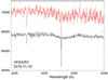 |
Fig. 1 Small region of the spectrum of the HD 024263 sightline obtained with the aid of the UVES pipeline (upper line, in red) and with our own interactive analysis system DECH (lower line, in black). The weak feature shortward of the CH+ line is the feature of 13CH+. |
2.2 Archive spectra
In addition to the 100 stars observed by us with UVES, we have found high-resolution spectra of 86 other sightlines. Seventeen UVES spectra were taken in the context of the EDIBLES survey (Cox et al. 2017), which covers almost the entire optical wavelength range from 320 to 1000 nm with an S/N exceeding 500 per pixel. Two spectra were taken from existing data (co-author Galazutdinov) of the 1.0 m Zeiss Special Astrophysical Observatory of the Russian Academy of Sciences and BOES at the 1.8 m Bohyunsan Optical Astronomy Observatory in Korea (Kim et al. 2007). Eighteen spectra were taken from ELODIE (Moultaka et al. 2004), FEROS (Kaufer et al. 1999), SOPHIE2, and ESO UVES archives, alternatively, their single- or multiple-cloud status was determined by a literature search using SIMBAD. These 36 sightlines with archive spectra are provided in Table 1. We found additional publicly available UVES and FEROS spectra for 50 stars that include the K I line. They are presented in Table 2.
2.3 WISE mid-IR imaging
In addition to optical high-resolution spectroscopy, we searched for mid-IR data, which provide dust emission signatures of the clouds. Mid-IR imaging is obtained with the Wide-field Infrared Survey Explorer (WISE, Wright et al. 2010) for all sources of Table 1. WISE3 mapped the sky at 3.4, 4.6, 12, and 22 μm (filters: W1, W2, W3, and W4) in 2010 with an angular resolution of 6.1″, 6.4″, 6.5″, and 12.0″ and a 5 σ point sourcesensitivities better than 0.08, 0.11, 1, and 6 mJy in the four bands, respectively.
3 Analysis of spectroscopic data and mid-IR imaging
In this section we present our spectral classification (Sect. 3.1) of the sample (Table 1) and measurements of radial velocities and equivalent widths (Sect. 3.2). In Sect. 3.3we derive column densities from the K I profile and identify the single-cloud sightlines. We then use the CH/CH+ line ratio to classify the environment of the clouds to be either cold or warm (Sect. 3.4), and in Sect. 3.5 we analyse WISE mid-IR images of our sightlines to constrain the location of the dust emission. We apply three different methods to estimate distances to the targets (Sect. 4).
HD 164747A and HD 164747B are separated by 3.4′′ and are not resolved by IUE. Both stars are covered in our UVES image. They are of same spectral type and show a different Doppler structure of Ca II lines. The DIB intensities are identical, and we therefore assume that the extinction curves are also identical. We removedHD 123335 (ID 59), HD 134591 (ID 62), HD 147331 (ID 70), and HD 151346 (ID 79) from our analysis because the lines are contaminated. We spectroscopically classified 136 stars of Table 1 and carried out the remaining analysis on 132 stars. The results are summarised in Table 3.
3.1 Spectral classification
Knowing the spectral type is important for estimating the reddening and spectral type-luminosity distance of a star. Our high-resolution spectra allow accurate measures of line intensities and profiles. We applied a two-step approach by estimating the spectral class of the stars following the procedure described and exemplified by Krełowski et al. (2018). The first step is based on the measured ratios of the H I, He I, and Mg II line strengths, as suggested by Walborn & Fitzpatrick (1990) and by the Stony Brook catalogue4. The position of OB standard stars in the Mg II/He I versus H I/He I plane was shown and tabulated by Krełowski et al. (2018). For example, in this scheme, a B6 star has Mg II/He ~ 0.9 and H I/He I ~ 20, while a B9.5 star shows Mg II/He I ~ 2.6 and H I/He I ≳ 70. The second step includes confirmation or correction of our initial spectral type classification through careful inspection of the high-resolution spectra of the considered stars. This includes interpretation of possible incompatibilities. In this second step, we inspect various line profiles of H I, He I, He II, C IV, Mg II, Si II, Si III, and Si IV. The detection of He II and C IV lines points to O type stars, while the Si IV line indicates an early-B star. That the strength ratio of the He I 4471 is higher than that of Mg II 4481 provides another indication for early B-type stars. At mid-B, the intensity of Si IV 4089 and Si III 4552 lines relative to that of Si II 4128-30 is the defining characteristic, while for late-B stars, the defining characteristic is the intensity of Mg II 4481 relative to that of He I 4471, according to Walborn (2008). Hydrogen Balmer line profiles provide evidence of a dwarf or a high-luminosity star. The similarity of lines such as the series of He I at 3965, 4009, 4026, 4121, 4144, 4169, 4388, 4437, 4713, 4923, and 5876 (Å) is characteristic for B-type stars when He II lines are absent. We also searched for signatures of multiple stellar components and binarity as apparent from the profile shapes. The intensities of weak stellar lines in fast rotators or in binaries are hard to estimate and create uncertainties in spectral-type determinations.
Our newly estimated spectral types and those previously given in the literature are listed in Cols. 7 and 8 of Table 1, respectively. For 89 out of the 136 stars, the two estimates agree to within one subclass. Fourteen stars were previously classified as B0-1 I-V while we identified them as O-type stars with 12 as O9 and the other between spectral type O4-8. Twenty-two stars of our sample appear to be spectroscopic binary stars, and 14 are associated with a cloud in SIMBAD. In the following paragraphs we discuss the discrepant cases and report the reason for our decision for a binary classification for some objects.
The typical signatures of O-type stars are the C IV 5801.3 and C IV 5811 lines, which are not seen in B-type stars. In O7 stars, the He I line near 4471.5 is as deep as He II 4541.6. In even hotter stars, the He II feature becomes stronger, while in late O-type stars, the He I line becomes dominant. For example, we classify Herschel 36 as O8V: the C IV lines are detected, but Mg II is barely visible, and He I is stronger than He II.
The luminosity class of a star can be estimated based on the H I line profiles. Our classifications were made by comparing the spectra of our targets with those given as standards by Walborn & Fitzpatrick (1990). Supergiants and bright giants (class I and II) show narrow H I lines, such as HD 046711 and HD 091943. Main-sequence stars (class IV and V) show broad H lines, such as HD 037903, HD 108927, and HD 147196.
Spectral types of several objects may be uncertain when they belong to a binary system, and the apparent binarity is revealed by double, blended profiles that are difficult to separate in the two components. We classify HD 315032 as an early B0 star because Mg II is barely visible. HD 156247 appears as a binary in He I, Mg II, and C II lines. The He I line profile appears likely blended in HD 315033 and in HD 161653, for which broad wings of H I lines and many O+ lines are detected. We classify HD 161653 as B3 II, although it was classified as B0.5 III by Valencic et al. (2004) and as B2 II by Houk (1982). The classification is uncertain because this star apparently is a binary, and the red component of He I seems broader than in Mg II. The hydrogen lines have broad wings, which is characteristic for dwarfs. However, if the star is of class IV, the spectral type-luminosity distance becomes only ~ 660 pc, while Gaia and Ca II measurements place it farther away than 1 kpc. In our class II, the spectral type-luminosity distance of HD 161653 becomes 1230 pc, which is very consistent with the other distance estimates (cf. Table 3).
Result summary.
3.2 Radial velocity and equivalent width measurements
We converted the spectra of Table 1 into normalised intensity versus heliocentric velocity for the profiles of the following spectral lines: Ti II 3383.8 Å, CN 3874.6 Å, Ca II K 3933.7 Å, CH 4300.3 Å, CH+ 4232.5 Å, Na I 5890 Å, and KI 7699 Å (see Figs. 2 and A.1). The broadest Ca II component seen in the spectrum of HD 062542 at 15.5 km s−1 is probably of stellar origin. We note that the profiles of Ti II and Ca II K lines often appear similar (Hunter et al. 2006) as are those of Na I and K I. In addition to these seven lines, we inspected other lines such as Ca I 4227 Å and DIBs covered in the observed wavelength range of our observations, finding that they had often low S/N, or are frequently saturated, like Na I 5895.9 Å. In addition to the heliocentric velocities, we also measured the equivalent widths for the Ca II H and K doublets, as given in Cols. 3 and 4 of Table 3. Interstellar lines often do not show the same radial velocities and appear in three distinct families. The radial velocity of (a) K I and CH commonly coincides nearly perfectly, and likely also with CN, while (b) CH+ frequently shows a shift. (c) The Ca II lines quite frequently show very complex Doppler structure, in contrast to other interstellar lines, while Ca II and Ti II show similar profiles. DIBs seem to originate in clouds following K I (Galazutdinov et al. 2000).
3.3 Identification of single-cloud sightlines
We classified the appearance of the radial velocity profiles of Ca II K, Na I, and K I as single (S) or multiple (M) component sightlines. The results are given in Cols. 8–10 of Table 3. The saturated Na I lines, for which a classification was not possible, are marked by a hyphen. We find that the K I line is particularly suited for the S or M classification. The K I profile is fit by a multiple-component Voigt function using the position and column density as free parameters; in order to estimate the column density, we applied the apparent optical depth method described by Savage & Sembach (1991) as implemented in DECH. The best-fit parameters to the K I profiles are given in Cols. 4 (position) and 6 (column density) in Table 2 and in Cols. 12 and 13 in Table 3, respectively.We compared our estimates of the column densities of the K I line as derived by VAPID and DECH. Generally both methods agree very well however for lines that are observed close to saturation or resolution limits the systematic differences become significant. We found that for 81 of the 132 sightlines of Table 3 that allowedus to perform this analysis, the fit to the K I profile required multiple components, while 51 of these stars were fit by a single-component model. In addition, we found that 14 of the 50 stars of Table 2 are dominated by a single-component. In total there are 65 out of 186 stars that we classify as single-cloud sightline.
A number of objects have been observed in the K I and Ca I surveys by Welty & Hobbs (2001) and Welty et al. (2003), who used the UHRF or McDonald spectrographs offering resolution of 0.5 km s−1. These observations are consistent with our classifications of multiple-component sightlines. For example, the multiple-component sightline HD 023180 shows a very asymmetric K I profile in UVES and reveals four components between 10.5 and 14.9 km s−1 in the spectra by Welty et al. (2003). HD 027778 shows a double peak in K I in UVES, which is confirmed in the spectrum by Welty & Hobbs (2001), which shows four about equally strong components between 14.1 and 18.6 km s−1. More interestingly, HD 207198 and HD 209975 show multiple components in the Welty & Hobbs (2001) and Welty et al. (2003) spectra, butthese lines appear in ELODIE and SOPHIE spectra as a single-component. ELODIE and SOPHIE have about half the resolving power provided by UVES, which obviously is insufficient to characterise single-cloud sightlines. Nine spectra in our sample observed at similarly low resolution therefore cannot be classified. These stars are marked LR in Table 3. Three stars have decent S/N spectra in Welty & Hobbs (2001) and Welty et al. (2003) and are in common to our single-cloud sightlines: HD 147933 and HD 149757 show at 0.5 km s−1 resolution significant fine structure in the K I line, while towards HD 147165 the second strongest component is a factor two fainter. Recently, Welty et al. (2020) finds that most of the material towards HD 062542 resides indeed in a single narrow velocity component. The ultra-high resolution spectra often exhibit fine structures in lines that appear to be single when observed at resolution of 1.5 km s−1 (Welty 2014). In total, we found that in our terminology 65 of the 186 stars of this investigation appear as single-cloud sightlines. Of these, about half have previously been identified as such by Sembach et al. (1993), Ensor et al. (2017), Siebenmorgen et al. (2018).
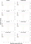 |
Fig. 2 UVES-derived heliocentric velocity profiles in Ti II 3383.8 Å (dark green), CN 3874.6 Å (magenta), CH 4300.3 Å (red), CH+ 4232.5 Å (blue), K I 7699 Å (green), Ca II K 3933.7 Å (orange), and Na I D2 5889 Å (brown). Single-cloud sightlines are marked “single”. For the remaining spectra, see Fig. A.1. |
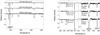 |
Fig. 3 Spectral features of the rotational R1, R0, and P1 transitions of cyanogen (CN) near 3875 Å (left), the CH+ 4232.5 Å and CH A-X 4300.3 Å transition (middle), and DIBs at 5780 Å and 5797 Å (right panel) for the three single-cloud sightlines HD 112607, HD 110715, and HD 030123. The CH/CH+ line intensityratio, E(B−V), distance, and some other lines are labelled. |
3.4 Cloud environment
Diffuse clouds show significant variations in their physical conditions depending on their density, the strength of the radiation field, the cosmic-ray intensity, and the presence or absence of shocks. The strength of simple radicals such as CN, CH, and CH+ and of DIBs are known to vary from cloud to cloud (Krelowski & Walker 1987). The presence of CH+ gives particular insights into the environmental condition of the clouds. CH+ is produced in media that are heated by a warm shock wave or a strong UV field, and it is rapidly destroyed by collisions with H, H2, and e− (Morris et al. 2016). The carriers of broad DIBs such as the 5780 Å band are more abundant when simple radicals are destroyed. This seems to occur in strongly irradiated warm clouds where CN is rarely seen. Regions showing weak ionisation with line intensity ratios CH/CH+ ≳ 1 appear to be connected to low-irradiation cold environments (Krełowski et al. 2019b), and the CN line is detected there. We show this result in Fig. 3 for HD 112607, HD 110715, and HD 030123, in which CN is detected and the cloud is cold (CH/CH+ ≳ 1), and in Fig. 4 for HD 146285, HD 148579, and HD 287150, in which CN is not detected and the cloud environment is warm (CH/CH+ < 1). This finding has been reported for five of our stars5 by Pan et al. (2005), where CH and CN column densities for moderately high-density gas (n > 30 cm−3) correlate and no CN is detected in low-density regions showing CH+.
The strength of the lines and DIBs is further discussed by Weselak et al. (2008) and Krełowski et al. (2019b). We have inspected the CH A-X 4300.3 Å,CH+ 4232.5 Å, andthe CN 3874.6 Å line in spectra of our sample (see Figs. 2 and A.1). The wavelength ranges of these lines are included in the spectra of 109 of our stars. Thirteen of them have a low S/N in CH and CN. In five stars, the CH lines were not detected. Three multiple-component sightlines show significant velocity shifts between the lines and were excluded from the analysis. This leaves us with 88 spectra. In six of them, CH and CN are split into two clearly separated velocity components, and because of the multiple-component sightlines, we were able to measure 97 ratios of CH/CH+ with or without a detection of CN lines. For these, we report in Col. 14 of Table 3 thirty-nine warm clouds (CH/CH+ < 1) in which the CN line is not detected, labelled w-CN; 54 cold clouds (CH/CH+ ≳ 1) in which the CN line is detected, labelled c+CN; and only four warm clouds in which CN is detected, labelled w+CN. The CN line is detected in all clouds labelled “cold”.
Data in CH and CN bands are available in 39 out of 51 single-cloud sightlines with spectra covering these features (Table 3). For these, CN is detected in 23 out of 37 single clouds that are classified as cold. Except in HD 156247, CN is missing in all other 14 single clouds that are classified as warm. When the cloud is close to the OB star, it should be warm. Clouds of single-cloud sightlines are cold and are predominantly located far away from the star in the cold ISM.
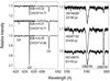 |
Fig. 4 Spectra of the CH+ 4232.5 Å and CH 4300.3 Å transition (left) and DIBs at 5780 Å and 5797 Å (right panel) for the three single-cloud sightlines HD 146285, HD 148579, and HD 287150. The CH/CH+ ratio, E(B−V) reddening, distance, and Ca I line are labelled. |
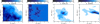 |
Fig. 5 WISE images in filter W4 (~ 22 μm) centred on stars of different morphological types. From left to right: HD 023180 (type a), HD 047107 (type b), HD 281159 (type c), and HD 046202 (type d). Fluxes levels are measured in mJy. |
3.5 Analysis of mid-IR imaging
We complemented our spectroscopic analysis using archive mid-IR imaging to assess the nature of the cloud environment. Dust is heated by UV and optical stellar light and re-emits the absorbed energy at infrared (IR) wavelengths. Inspecting the appearance of our sources in the mid-IR may allow us to constrain the location of the dust cloud(s) along the sightline that is either nearby the star in a circumstellar envelope or farther away in the diffuse ISM. We studied the connection of star and dust emission along the sightlines by inspecting the morphology of mid-IR images provided by WISE in a 5′ × 5′ field centred on our stars.
The observed mid-IR fluxes are dominated either by star or dust emission. When the flux is dominated by dust emission, it is likely resolved in the WISE W3 and W4 bands. This can be demonstrated by computing the dust emission of a circumstellar dust envelope of a mixture of large 600 nm sized carbon and silicate grains that are heated by a typical B-type star of our target list. The star has a luminosity of 104 L⊙ and temperature of 20 000 K. The shell has an inner boundary set by dust evaporation at temperature ~ 1500 K and an outer radius of 1 pc. For a dust envelope with a constant density and dust mass of 0.8 M⊙ the total optical depth τV = 1. In this shell dust becomes warmer than 80 K up to distances of a few 1017 cm. This envelope may be detected with the spatial resolution of WISE6 up to 1 kpc distance, and more so when the emission, for example in W3, is dominated by very small (nanometre)particles such as polycyclic aromatic hydrocarbons, e.g. Siebenmorgen (1993), Krügel (2008). It may be considered that dust clouds have much higher optical depth than estimated from adopting the AV of the sightline to the star (Table 1). In this case, the clouds could be heated by embedded stars. Because stars like this are unseen in the near-IR but the optical depth must be very high (AV ≥ 10 mag) in the mid-IR, a scenario for the given AV of our sightlines is unlikely.
We classified the morphology of the WISE images and distinguished the following cases: (a) images without dust emission signatures. The WISE image at the position of the star appears point-like, and is brighter in W1 and W2 than in W3 and W4, where the star is sometimes not even detected. (b) Image background is enhanced. The emission near the star shows a somewhat enhanced diffuse background component in W3 and even more so in W4. (c) A cloud is detected. The star is located in or seems within less than 1′ associated with a bright extended and often ellipsoidal dust cloud. The clouds are often brighter in the W3 and more so in the W4 band than in the W1 and W2 bands. (d) A distant dust lane or cloud is detected more than 1′ away from the star, and is likely not associated with the star. The dust lane often extends across the full WISE image. The dust lane or cloud is often brighter in W3 and more so in W4 than in W1 and W2.
Typical examples of our classification of the emission morphology as seen by WISE in filter W4 are shown in Fig. 5 for HD 023180 (case a), HD 047107 (case b), HD 281159 (case c), and HD 046202 (case d). In the W4 (22 μm) image of HD 023180, two point sources are detected, one lies at the position of the star. In HD 47107 the star is detected and surrounded by some diffuse enhanced background. HD 281159 is detected near the centre of a cloud and surrounded by a structure that is bright in W4, visible in W1 and W2, but not detected in W3. The star HD 046202 is not detected, but a cloud 2′ W of it is visible. Other remarkable structures are seen for HD 172028, which is inside a cloud that is bright in all bands. HD 155756 shows a nearby cloud 1′ NE that is likely not associated with the star. HD 200775 shows two bright dust clouds and one around the star. Of the 132 objects with a WISE classification in Col. 15 of Table 3, 83 (63%) fall in category a, 20 (15%) in category b, 14 (11%) in category c, and 14 (11%) in category d. The distribution is similar for the 51 single-cloud sightlines: WISE images exist for all these stars, and 32 (63%) of them are in category a, 9 (15%) in category b, 2 (4%) in category c, and 9 (17%) in category d.
An extended dust halo or circumstellar shell that might contribute significantly to the total dust column density along the sightline is detected in a minority of our sample. This is category c, which includes only 10% of the stars. Therefore dust along our sightlines seems predominantly (90%) located in the diffuse ISM, at least the clouds are not detected by dust emission within a 1′ neighbourhood to the stars.
4 Distance estimates
We have derived the distances of our sample of early-type stars using three different methods: (i) Gaia parallax (DGaia), (ii) spectral type-luminosity (DSpL), and (iii) the amount of interstellar matter derived from the Ca II (H, K) doublet (DCa II), as proposed by Megier et al. (2005).
For the first method, the geometric distances DGaia were taken from Bailer-Jones et al. (2018). They are based on the second Gaia data release, where an inference procedure is used, which does not consider the physical properties of the stars. Furthermore, the uncertainty of parallax measurements increases with increasing distance to the star.
In the second method, the spectral type-luminosity distances DSpL were obtained from the spectral type and luminosity using the spectral classification of Sect. 3.1 and dust extinction given in Table 1. Spectral type-luminosity distances depend on the correct identification of spectral type and luminosity class of a star. A difference of one spectral subclass in OB stars changes the derived stellar temperature already by 10%, implying an error in the distance of 40%. This method also requires a correction for dust extinction with its own uncertainties, e.g. Krügel (2009), Scicluna & Siebenmorgen (2015). Unresolved binaries, which are common among early-type stars, result in errors in the spectral type and affect the estimate of the spectral type-luminosity distance.
The distance estimates DCa II were obtained in the third method using the relation between interstellar absorption to distance that has been studied by Struve (1928) and more recently by Smoker et al. (2006). This method works well when the absorbing material is relatively uniformly distributed, and within the Galactic plane. Galazutdinov (2005) showed that the Ca II is a better distance indicator than K I, Na I or the reddening E(B−V). Megier et al. (2009) reported a simple relation between the equivalent width of the Ca II (H, K) doublet and the distance DCa II. Large-scale structures and dependences on galactic latitude, local enhancements in the Ca II column density, likely related to stellar clusters and associations, and a frequent saturation of the Ca II line limit the accuracy of the method. Therefore we used our equivalent width measurements of the Ca II (H, K) doublet (Cols. 3–4 of Table 3) and used the formulae of Megier et al. (2009) to compute the distance DCa II. Distance estimates derived from the three methods for the 132 stars of our sample are given in Cols. 5–7 of Table 3.
The relationships between the distance estimates DGaia, DCa II, and DSpL derived in Sect. 4 are shown in Fig. 6. Binaries and stars associated with clouds are ignored. For a reasonable DCa II estimate the ratio of the equivalent width of the Ca II H and K doublet is EW(H)∕EW(K) > 1.32. We considered stars with all three estimates measured at >3σ confidence and excluded binaries. This returned samples that included 59 pairs of distance estimates that correlate with Pearson’s coefficient ρ(DGaia, DCa II) ~ 0.74, ρ(DGaia, DSpL) ~ 0.89, and ρ(DCa II, DSpL) ~ 0.82. At short distances, DGaia ≤ 2 kpc, there are 48 pairs that are correlated more strongly (ρ ≳ 0.87), while at larger distance, DGaia > 2 kpc, 11 pairs remain and the correlation with Gaia distances breaks down.
In Fig. 6 we also show 232 distance estimates derived from the Ca II H, K doublet measurements at > 3σ confidence and EW(H)∕EW(K) > 1.32 by Megier et al. (2009). They show similarscatter, and their DCa II estimates are correlated at DGaia < 6 kpc with ρ = 0.7, and a subsample at DGaia ≤ 2 kpc is correlated with ρ = 0.83. The sample of Megier et al. (2009) and our sample have 17 stars in common. The equivalent width of the Ca II H, K generally agrees to better than 4%, with three exceptions: HD 027778, HD 099872, and HD 141318. For these stars the equivalent width shows larger variations, so that the derived Ca II distances differ by more than 20%. When it was available, we used the UVES-derived DCa II estimates because thisinstrument provides the highest resolving power. Megier et al. (2009) applied hipparcos (ESA 1997) data to derive their DCa II formulae. We show the two data samples in top panel of Fig. 6. No significant trend in the equivalent width of the Ca II (H, K) doublet with the parallax distance estimates is visible that would reduce the observed scatter.
Overall, we note a large variation of about a factor of two when different distance estimates of the same star are compared. Within this scatter, DCa II ~ DGaia while DCa II ~ 0.8 × DSpL, but the sparse statistics prevents firm conclusions. Figure 6 shows that the variation in the distances remains when subsamples of sightlines are built that are dominated by single or multiple clouds and warm or cold cloud environments. The reddening of our sample is not correlated with the Gaia distance either (ρ(E(B−V), DGaia) = 0.2).
We mark in Fig. 6 cases where the spectral type-luminosity and Ca II distances agree but the Gaia distance at low and high value of the parallax differs by more than a factor of three. For example, HD 050562 is in Gaia located far away at 3.4 kpc, while DCa II ~ DSpL ~ 1.1 kpc are closer by a factor three. On the other hand, HD 143054 is predicted to be at 300 pc nearby when Gaia is used, while DCa II ~ DSpL ≳ 1.1 kpc, which is a factor four farther away. The distances of HD 024263 derived from Gaia and spectral type-luminosity ratio are at ~ 220 pc, while DCa II estimates are at 670 pc, or finally, HD 110715 shows DCa II ~ DSpL ~ 530 pc, while DSpL ~ 270 pc. Further discrepancies can be identified in Table 3. No method can be favoured for individual stars over another method for deriving distances.
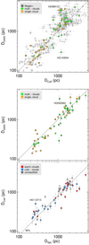 |
Fig. 6 Relation between distance estimates using Gaia parallax DGaia (Bailer-Jones et al. 2018), spectral type-luminosity DSpL, and the Ca II H, K doublet, DCa II. Squares (grey) represent the Ca II distances by Megier et al. (2009), and circles indicate the distances as listed in Table 3, with sightlines dominated by single-cloud (orange), multiple clouds (green), cold (blue), and warm (red) clouds, as labelled. |
5 Dark dust
The distance D of a star, its apparent mV and absolute magnitude MV, and the dust extinction along the sightline is connected by the photometric equation. Dust absorbs relatively more blue than red photons, so that the interstellar extinction is often exchanged by the term “reddening” and simplified to be given by AV = RV × EB-V. However, it was never proved that it is allowed to neglect any additional constant extinction that represents some neutral, grey, or as we call it, dark dust. The original form of the photometric equation by Trumpler (1930) includes in addition to the wavelength-dependent selective interstellar extinction also a constant CDark that represents dark dust,
 (2)
(2)
Trumpler (1930) estimated CDark ~ 0.2 mag kpc−1, which today appears a crude underestimate. He proposed “meteoric bodies”, and we claim grains of sizes larger than the wavelength of the obscured light to explain dark dust extinction. Several studies have claimed the detection of a dark dust component populated by ≳ 1 μm large grains.Dark dust is frequently found around circumstellar shells, e.g. Strom et al. (1971), Sitko et al. (1994), Lanz et al. (1995) or evolved stars, e.g. Apruzese (1974), Andriesse et al. (1978), Jura et al. (2001), Scicluna et al. (2015). This dark dust often occurs together with a total-to-selective extinction that is higher than the canonical value of Milky Way dust of RV ≳ 3.1 (Fitzpatrick et al. 2019). More recently, Krełowski et al. (2016) reported that the Ca II as well as VLBI parallax distances of the Orion Trapezium star HD 037020 differ from the spectral type-luminosity distance by a factor 2.5. They interpreted this as being due to ADark = 1.8 mag dark dust extinction in front of the star. Dark dust has also been detected in the general field by Skórzyński et al. (2003). They reported that towards some OB stars that are located within 400 pc of the solar neighbourhood, the intrinsic absolute magnitudes are too faint so that the derived spectral type-luminosity distances are significantly overestimated when compared to hipparcos distances. This discrepancy is explained by a few magnitudes of dark dust extinction in the ISM.
We considered stars of Table 3 at Gaia distances ≲ 2 kpc, measured at > 4σ confidence, and excluded binaries, as reported in Table 1. For 9 out of 77 of such stars the spectral type-luminosity distance differs significantly by more than ± 50% from the Gaia distance. This interval includes eight stars with DSpL ≳ 1.5 × DGaia (Table 4) and one peculiar star, HD 112954, for which DGaia ~ 2.25 DSpL. When these eight stars are excluded, the scatter in DSpL∕DGaia is reduced to ~22%. We find first that dark dust sightlines appear most frequently in the field. Our sample includes only one star, HD 037903, with which a dust cloud can be associated in WISE imaging (Sect. 3.5). This star illuminates the bright reflection nebula NGC 2023 in Orion and shows vibrationally excited interstellar H2, which is indicative of a photodissociation region around the star (Meyer et al. 2001; Gnaciński 2011).
We also find that the extinction of light by dark dust occurs in the cold ISM. At least all dark dust sightlines detected by us are associated with cold cloud environments (Sect. 3.4).
Finally, dark dust sightlines show predominantly flat extinction curves. Six such stars lie at RV ≳ 3.8. Flat extinction curves are associated with large grains.
We estimated the amount of dark extinction under the assumption that the Gaia distance is precise and the luminosity L of the star is correctly derived by our spectral classification. The observed flux is given by
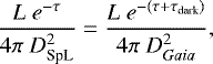 (3)
(3)
hence 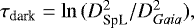 which amounts to typically 1−3 mag of dark dust extinction (Table 4). High-precision extinction measurements in the near-IR or at even longer wavelengths are required for a clear identification of large particles that remain hidden in the dark dust component of the ISM.
Dark dust detections.
6 Summary and conclusions
We have argued here that our interpretation of the extinction and polarisation of the interstellar medium is strongly biased by the fact that multiple interstellar clouds may be present along any line of sight. Recently, we have shown that when the analysis is limited to what we call single-cloud sightlines, new relationships appear between the observing characteristics of extinction and polarisation and the physical properties of the dust. These relations are hidden in multiple-cloud sightlines where interstellar lines are Doppler-split, while single-cloud sightlines are suitable to investigate the pristine nature of interstellar material. Unfortunately, while hundreds of extinction and polarisation curves have been measured for the ISM, the number of single-cloud sightlines that have been investigated is still very limited. Siebenmorgen et al. (2018) argued that data for detailed dust modelling are available for only eight single-cloud sightlines. To overcome this observational bias, we performed an extensive survey of high-resolution spectra of reddened OB stars for which the far-UV extinction curve has been measured by IUE or FUSE. We compiled a sample of 186 high-resolution spectra of such stars, 100 of which were observed by us using the UVES instrument of the ESO Very Large Telescope. Archive spectra with a broad wavelength coverage for another 36 sightlines where retrieved from various archives, as well as 50 accompanying UVES narrow-band archive spectra that include the K I line. All sightlines for which UVES raw data were available were reprocessed by us with our interactive analysis package DECH.
Dust properties are assumed to vary on a large scale, typically when dust clouds are separated by several 10s or 100s of pc, whereas within a single-cloud, the mean characteristics of dust remain. This paper was tailored to detect single-cloud dominated sightlines that can be used for further investigations of the dust characteristics in the diffuse ISM. In this context, we assign the term single-cloud sightline when the observed interstellar lines observed at ~ 4 km s−1 (FWHM) resolution showed one dominating Doppler component. In this way, we realised that interstellar lines come in families of distinct radial velocities with K I coinciding with CH, while CH+ is often shifted, and Ca II and Ti II show similar and more complex structures. These offsets in the velocity profiles, as well as local small-scale variations and details in the cloud morphology, were not considered. Comparisons of our stars that are in common with previous ultra-high resolution spectra by Welty & Hobbs (2001) and Welty et al. (2003), for example, confirmed our assignment of multiple-component sightlines. Such spectra often exhibit fine structures in lines that appear to be single when observed at resolution of 1.5 km s−1 (Welty 2014). Nevertheless, the comparison also demonstrated that lower resolution spectra at > 4 km s−1 (FWHM) are insufficient for this classification. We identified a sample of 65 single-cloud sightlines in the 186 high-resolution spectra, the majority of which were previously unknown.
In 97 sightlines we detected CH and CH+, and we used their strength ratio for the classification into warm (line ratio CH/CH+ < 1) or cold (CH/CH+ > 1) clouds. In all 52 cold clouds we did detect CN, while we did not detect it in 32 out of 36 warm clouds. Most of the clouds are cold and located sufficiently far away from the heating source in the cold diffuse ISM. We inspected the WISE 3 − 22 μm emission morphology of our clouds. They appear predominantly stellar, while dust emission that is associated with the star is detected in only 10% of the cases. Therefore we exclude a circumstellar nature of the observed reddening for most cases, and the extinction towards our stars is due to dust located in the diffuse ISM.
The high resolving power of our data has allowed us to accurately measure the Mg II/He I and He I/H I line intensity ratios, which were used in addition to other features to revisit the spectral classification of our targets. In the majority of cases (89 of 136), we confirmed previous assignments found in the literature, but for 47 of 136 stars, our revision of spectral type was substantial. We identified binary systems in 22 sightlines. We used our revised classification to compute the spectral type-luminosity distance of the stars. We also measured the equivalent width of the Ca II H and K doublet and estimated the spectroscopic distance of the stars. We compared the two distance estimates to the Gaia parallaxes. Overall, the scatter in the distance estimates is large at ~ 40%. In some cases, only one of the three distances differs heavily from the others. Sometimes, to agree with Gaia, spectroscopic estimates require an unacceptably low luminosity of the stars. We cannot favour one method over others to derive the distances.
Finally, we detected a hidden dust population that amounts to a 1–3 mag extinction in the ISM. We called this dark dust. For these stars, the spectral type-luminosity distances are significantly larger than derived by Gaia. Dark dust predominantly appears in the cold ISM with flat extinction curves. Dark dust does not show a wavelength-dependent absorption of stellar light in the optical. It is presumably made of very large ≳ 1 μm sized grains.For a direct identification of such dark dust particles, high-precision extinction measurements in the near-IR or at even longer wavelength are required.
In a forthcoming paper we will detail our stellar classifications and we will use the sample of 65 single-cloud sightlines to investigate the polarisation properties of the interstellar medium, and we will search for correlations between diffuse interstellar bands, atomic and molecular lines, and other properties of ISM dust such as the reported dark dust component.
Acknowledgements
We are greatful to the referee for pointing us to the UHRF data and valuable comments by Daniel Welty. This research is based on data obtained from the ESO Science Archive Facility and in particular on observations collected under ESO observing programme ID 0102.C-0040. Additionally, data from the following ESO programme IDs was used in this paper: 065.I-0526(A), 065.N-0378(A), 066.B-0320(A), 071.C-0513(C), 073.C-0337(A), 073.D-0024(A), 076.C-0431(A), 096.D-0008(A), 099.C-0637(A), 194.C-0833(A). We also used spectra retrieved from the ELODIE and SOPHIE archives at Observatoire de Haute-Provence (OHP) (available at atlas.obs-hp.fr/elodie and atlas.obs-hp.fr/sophie). This research has also made use of the SIMBAD database, operated at the CDS, Strasbourg, France. G.A.G. and J.K. acknowledge the financial support of the Chilean fund CONICYT grant REDES 180 136. J.K. acknowledge the financial support of the Polish National Science Centre, Poland (2017/25/B/ST9/01524) for the period 2018–2021.
Appendix A Additional tables and figures
Complete entries of Tables 1–3 are provided in Tables A.1–A.3, respectively. The remaining figures of the UVES-derived velocity profiles are displayed in Fig. A.1.
Study sample sorted by HD number.
UVES and FEROS archive spectra covering the K I line.
Result summary.
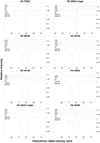 |
Fig. A.1 Heliocentric velocity profiles of Ti II 3383.8 Å (dark green), CN 3874.6 Å (magenta), CH 4300.3 Å (red), CH+ 4232.5 Å (blue), K I 7699 Å (green), Ca II K 3933.7 Å (orange), and Na I D2 5889 Å (brown). Single-cloud sightlines are marked “single”. |
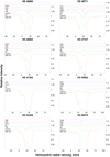 |
Fig. A.1 continued. |
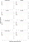 |
Fig. A.1 continued. |
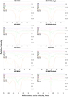 |
Fig. A.1 continued. |
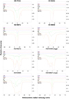 |
Fig. A.1 continued. |
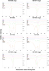 |
Fig. A.1 continued. |
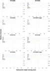 |
Fig. A.1 continued. |
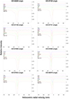 |
Fig. A.1 continued. |
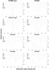 |
Fig. A.1 continued. |
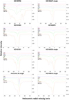 |
Fig. A.1 continued. |
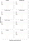 |
Fig. A.1 continued. |
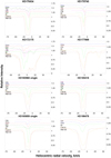 |
Fig. A.1 continued. |
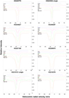 |
Fig. A.1 continued. |
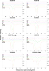 |
Fig. A.1 continued. |
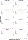 |
Fig. A.1 continued. |
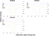 |
Fig. A.1 continued. |
References
- Andriesse, C. D., Donn, B. D., & Viotti, R. 1978, MNRAS, 185, 771 [NASA ADS] [Google Scholar]
- Apruzese, J. P. 1974, ApJ, 188, 539 [NASA ADS] [CrossRef] [Google Scholar]
- Bagnulo, S., Fossati, L., Kochukhov, O., & Landstreet, J. D. 2013, A&A, 559, A103 [NASA ADS] [CrossRef] [EDP Sciences] [Google Scholar]
- Bagnulo, S., Cox, N. L. J., Cikota, A., et al. 2017, A&A, 608, A146 [NASA ADS] [CrossRef] [EDP Sciences] [Google Scholar]
- Bailer-Jones, C. A. L., Rybizki, J., Fouesneau, M., Mantelet, G., & Andrae, R. 2018, AJ, 156, 58 [NASA ADS] [CrossRef] [Google Scholar]
- Barlow, M. J., Crawford, I. A., Diego, F., et al. 1995, MNRAS, 272, 333 [NASA ADS] [CrossRef] [Google Scholar]
- Chini, R., & Kruegel, E. 1983, A&A, 117, 289 [NASA ADS] [Google Scholar]
- Cox, N. L. J., Cami, J., Farhang, A., et al. 2017, A&A, 606, A76 [NASA ADS] [CrossRef] [EDP Sciences] [Google Scholar]
- Crane, P., Lambert, D. L., & Sheffer, Y. 1995, ApJS, 99, 107 [NASA ADS] [CrossRef] [Google Scholar]
- Crawford, I. A. 2002, MNRAS, 334, L33 [NASA ADS] [CrossRef] [Google Scholar]
- Dekker, H., D’Odorico, S., Kaufer, A., Delabre, B., & Kotzlowski, H. 2000, Proc. SPIE Conf. Ser., 4008, 534 [Google Scholar]
- Diego, F., Fish, A. C., Barlow, M. J., et al. 1995, MNRAS, 272, 323 [NASA ADS] [CrossRef] [Google Scholar]
- Elmegreen, B. G. 2002, ApJ, 564, 773 [NASA ADS] [CrossRef] [Google Scholar]
- Ensor, T., Cami, J., Bhatt, N. H., & Soddu, A. 2017, ApJ, 836, 162 [NASA ADS] [CrossRef] [Google Scholar]
- ESA 1997, The HIPPARCOS and TYCHO Catalogues. Astrometric and Photometric Star Catalogues Derived from the ESA hipparcos Space Astrometry Mission (Noordwijk, The Netherlands: ESA Publications Division), 1200 [Google Scholar]
- Falgarone, E., Phillips, T. G., & Walker, C. K. 1991, ApJ, 378, 186 [NASA ADS] [CrossRef] [Google Scholar]
- Falle, S. A. E. G., & Hartquist, T. W. 2002, MNRAS, 329, 195 [NASA ADS] [CrossRef] [Google Scholar]
- Fan, H., Hobbs, L. M., Dahlstrom, J. A., et al. 2019, ApJ, 878, 151 [NASA ADS] [CrossRef] [Google Scholar]
- Field, G. B. 1974, ApJ, 187, 453 [NASA ADS] [CrossRef] [Google Scholar]
- Fitzpatrick, E. L., & Massa, D. 1990, ApJS, 72, 163 [NASA ADS] [CrossRef] [Google Scholar]
- Fitzpatrick, E. L., & Massa, D. 2007, ApJ, 663, 320 [NASA ADS] [CrossRef] [EDP Sciences] [Google Scholar]
- Fitzpatrick, E. L., Massa, D., Gordon, K. D., Bohlin, R., & Clayton, G. C. 2019, ApJ, 886, 108 [NASA ADS] [CrossRef] [Google Scholar]
- Galazutdinov, G. 2005, J. Korean Astron. Soc., 38, 215 [NASA ADS] [CrossRef] [Google Scholar]
- Galazutdinov, G. A., Krełowski, J., & Musaev, F. A. 2000, MNRAS, 315, 703 [NASA ADS] [CrossRef] [Google Scholar]
- Gnaciński, P. 2011, A&A, 532, A122 [NASA ADS] [CrossRef] [EDP Sciences] [Google Scholar]
- Gordon, K. D., Cartledge, S., & Clayton, G. C. 2009, ApJ, 705, 1320 [NASA ADS] [CrossRef] [Google Scholar]
- Heger, M. L. 1922, Lick Observ. Bull., 10, 141 [NASA ADS] [CrossRef] [Google Scholar]
- Hong, S. S., & Greenberg, J. M. 1980, A&A, 88, 194 [NASA ADS] [Google Scholar]
- Houk, N. 1982, Michigan Catalogue of Two-dimensional Spectral Types for the HD Stars (Havard: MCTS Book) [Google Scholar]
- Houk, N., & Swift, C. 1999, Michigan Spectral Survey, 5, 0 [Google Scholar]
- Howarth, I. D., Price, R. J., Crawford, I. A., & Hawkins, I. 2002, MNRAS, 335, 267 [NASA ADS] [CrossRef] [Google Scholar]
- Hunter, I., Smoker, J. V., Keenan, F. P., et al. 2006, MNRAS, 367, 1478 [CrossRef] [Google Scholar]
- Jura, M., Webb, R. A., & Kahane, C. 2001, ApJ, 550, L71 [NASA ADS] [CrossRef] [Google Scholar]
- Kaufer, A., Stahl, O., Tubbesing, S., et al. 1999, The Messenger, 95, 8 [Google Scholar]
- Kim, K.-M., Han, I., Valyavin, G. G., et al. 2007, PASP, 119, 1052 [Google Scholar]
- Klein, R. I., McKee, C. F., & Colella, P. 1994, ApJ, 420, 213 [NASA ADS] [CrossRef] [Google Scholar]
- Krelowski, J., & Walker, G. A. H. 1987, ApJ, 312, 860 [NASA ADS] [CrossRef] [Google Scholar]
- Krełowski, J., Snow, T. P., Seab, C. G., & Papaj, J. 1992, MNRAS, 258, 693 [NASA ADS] [CrossRef] [Google Scholar]
- Krełowski, J., Beletsky, Y., Galazutdinov, G. A., et al. 2010, ApJ, 714, L64 [NASA ADS] [CrossRef] [Google Scholar]
- Krełowski, J., Galazutdinov, G. A., Bondar, A., & Beletsky, Y. 2016, MNRAS, 460, 2706 [NASA ADS] [CrossRef] [Google Scholar]
- Krełowski, J., Strobel, A., Galazutdinov, G. A., Musaev, F., & Bondar, A. 2018, Acta Astron., 68, 285 [Google Scholar]
- Krełowski, J., Strobel, A., Galazutdinov, G. A., Bondar, A., & Valyavin, G. 2019a, MNRAS, 486, 112 [CrossRef] [Google Scholar]
- Krełowski, J., Galazutdinov, G., & Bondar, A. 2019b, MNRAS, 486, 3537 [CrossRef] [Google Scholar]
- Krügel, E. 2008, An Introduction to the Physics of Interstellar Dust b6 (Amsterdam: IOP Press) [Google Scholar]
- Krügel, E. 2009, A&A, 493, 385 [NASA ADS] [CrossRef] [EDP Sciences] [Google Scholar]
- Lanz, T., Heap, S. R., & Hubeny, I. 1995, ApJ, 447, L41 [NASA ADS] [CrossRef] [Google Scholar]
- Lauroesch, J. T., Meyer, D. M., & Blades, J. C. 2000, ApJ, 543, L43 [CrossRef] [Google Scholar]
- McGuire, B. A. 2018, ApJS, 239, 17 [Google Scholar]
- Megier, A., Strobel, A., Bondar, A., et al. 2005, ApJ, 634, 451 [NASA ADS] [CrossRef] [Google Scholar]
- Megier, A., Strobel, A., Galazutdinov, G. A., & Krełowski, J. 2009, A&A, 507, 833 [NASA ADS] [CrossRef] [EDP Sciences] [Google Scholar]
- Meyer, D. M., Lauroesch, J. T., Sofia, U. J., Draine, B. T., & Bertoldi, F. 2001, ApJ, 553, L59 [NASA ADS] [CrossRef] [Google Scholar]
- Morris, P. W., Gupta, H., Nagy, Z., et al. 2016, ApJ, 829, 15 [NASA ADS] [CrossRef] [EDP Sciences] [Google Scholar]
- Moultaka, J., Ilovaisky, S. A., Prugniel, P., & Soubiran, C. 2004, PASP, 116, 693 [NASA ADS] [CrossRef] [Google Scholar]
- Pan, K., Federman, S. R., Sheffer, Y., & Andersson, B. G. 2005, ApJ, 633, 986 [NASA ADS] [CrossRef] [Google Scholar]
- Price, R. J., Crawford, I. A., & Barlow, M. J. 2000, MNRAS, 312, L43 [NASA ADS] [CrossRef] [Google Scholar]
- Savage, B. D., & Sembach, K. R. 1991, ApJ, 379, 245 [NASA ADS] [CrossRef] [Google Scholar]
- Scicluna, P., & Siebenmorgen, R. 2015, A&A, 584, A108 [NASA ADS] [CrossRef] [EDP Sciences] [Google Scholar]
- Scicluna, P., Siebenmorgen, R., Wesson, R., et al. 2015, A&A, 584, L10 [NASA ADS] [CrossRef] [EDP Sciences] [Google Scholar]
- Sembach, K. R., Danks, A. C., & Savage, B. D. 1993, A&AS, 100, 107 [NASA ADS] [Google Scholar]
- Siebenmorgen,R. 1993, ApJ, 408, 218 [NASA ADS] [CrossRef] [EDP Sciences] [Google Scholar]
- Siebenmorgen,R., Voshchinnikov, N. V., Bagnulo, S., et al. 2018, A&A, 611, A5 [NASA ADS] [CrossRef] [EDP Sciences] [Google Scholar]
- Sitko, M. L., Halbedel, E. M., Lawrence, G. F., Smith, J. A., & Yanow, K. 1994, ApJ, 432, 753 [NASA ADS] [CrossRef] [Google Scholar]
- Skórzyński, W., Strobel, A., & Galazutdinov, G. A. 2003, A&A, 408, 297 [NASA ADS] [CrossRef] [EDP Sciences] [Google Scholar]
- Smoker, J. V., Lynn, B. B., Christian, D. J., & Keenan, F. P. 2006, MNRAS, 370, 151 [NASA ADS] [CrossRef] [Google Scholar]
- Smoker, J., Haddad, N., Iwert, O., et al. 2009, The Messenger, 138, 8 [NASA ADS] [Google Scholar]
- Spitzer, L. 1978, Physical Processes in the Interstellar Medium (Hoboken: WILEY VCH Verlag) [Google Scholar]
- Strom, K. M., Strom, S. E., & Yost, J. 1971, ApJ, 165, 479 [NASA ADS] [CrossRef] [Google Scholar]
- Struve, O. 1928, ApJ, 67, 353 [NASA ADS] [CrossRef] [Google Scholar]
- Tolstoy, E., Venn, K. A., Shetrone, M., et al. 2003, AJ, 125, 707 [NASA ADS] [CrossRef] [Google Scholar]
- Trumpler, R. J. 1930, PASP, 42, 214 [Google Scholar]
- Tull, R. G., MacQueen, P. J., Sneden, C., & Lambert, D. L. 1995, PASP, 107, 251 [NASA ADS] [CrossRef] [Google Scholar]
- Valencic, L. A., Clayton, G. C., & Gordon, K. D. 2004, ApJ, 616, 912 [NASA ADS] [CrossRef] [Google Scholar]
- Wada, K. 2008, ApJ, 675, 188 [NASA ADS] [CrossRef] [Google Scholar]
- Walborn, N. R. 2008, Rev. Mex. Astron. Astrofis. Conf. Ser., 33, 5 [NASA ADS] [Google Scholar]
- Walborn, N. R., & Fitzpatrick, E. L. 1990, PASP, 102, 379 [Google Scholar]
- Wegner, W. 2003, Astron. Nachr., 324, 219 [NASA ADS] [CrossRef] [Google Scholar]
- Welty, D. E. 2014, IAU Symp., 297, 153 [NASA ADS] [Google Scholar]
- Welty, D. E., & Crowther, P. A. 2010, MNRAS, 404, 1321 [NASA ADS] [Google Scholar]
- Welty, D. E., & Fitzpatrick, E. L. 2001, ApJ, 551, L175 [NASA ADS] [CrossRef] [Google Scholar]
- Welty, D. E., & Hobbs, L. M. 2001, ApJS, 133, 345 [NASA ADS] [CrossRef] [Google Scholar]
- Welty, D. E., Hobbs, L. M., & Kulkarni, V. P. 1994, ApJ, 436, 152 [NASA ADS] [CrossRef] [Google Scholar]
- Welty, D. E., Morton, D. C., & Hobbs, L. M. 1996, ApJS, 106, 533 [NASA ADS] [CrossRef] [Google Scholar]
- Welty, D. E., Hobbs, L. M., & Morton, D. C. 2003, ApJS, 147, 61 [NASA ADS] [CrossRef] [EDP Sciences] [Google Scholar]
- Welty, D. E., Sonnentrucker, P., Snow, T. P., & York, D. G. 2020, ApJ, 897, 36 [Google Scholar]
- Weselak, T., Galazutdinov, G. A., Musaev, F. A., & Krełowski, J. 2008, A&A, 484, 381 [NASA ADS] [CrossRef] [EDP Sciences] [Google Scholar]
- Wright, E. L., Eisenhardt, P. R. M., Mainzer, A. K., et al. 2010, AJ, 140, 1868 [Google Scholar]
Available upon request to G. Galazutdinov.
Images available at: https://irsa.ipac.caltech.edu/applications/wise/
HD 147888, HD 147933, HD 204827, HD 206267, and HD 207198.
A 6″ beam has a linear scale of 1017 cm at 1115 pc.
All Tables
All Figures
|
Fig. 1 Small region of the spectrum of the HD 024263 sightline obtained with the aid of the UVES pipeline (upper line, in red) and with our own interactive analysis system DECH (lower line, in black). The weak feature shortward of the CH+ line is the feature of 13CH+. |
| In the text | |
|
Fig. 2 UVES-derived heliocentric velocity profiles in Ti II 3383.8 Å (dark green), CN 3874.6 Å (magenta), CH 4300.3 Å (red), CH+ 4232.5 Å (blue), K I 7699 Å (green), Ca II K 3933.7 Å (orange), and Na I D2 5889 Å (brown). Single-cloud sightlines are marked “single”. For the remaining spectra, see Fig. A.1. |
| In the text | |
|
Fig. 3 Spectral features of the rotational R1, R0, and P1 transitions of cyanogen (CN) near 3875 Å (left), the CH+ 4232.5 Å and CH A-X 4300.3 Å transition (middle), and DIBs at 5780 Å and 5797 Å (right panel) for the three single-cloud sightlines HD 112607, HD 110715, and HD 030123. The CH/CH+ line intensityratio, E(B−V), distance, and some other lines are labelled. |
| In the text | |
|
Fig. 4 Spectra of the CH+ 4232.5 Å and CH 4300.3 Å transition (left) and DIBs at 5780 Å and 5797 Å (right panel) for the three single-cloud sightlines HD 146285, HD 148579, and HD 287150. The CH/CH+ ratio, E(B−V) reddening, distance, and Ca I line are labelled. |
| In the text | |
|
Fig. 5 WISE images in filter W4 (~ 22 μm) centred on stars of different morphological types. From left to right: HD 023180 (type a), HD 047107 (type b), HD 281159 (type c), and HD 046202 (type d). Fluxes levels are measured in mJy. |
| In the text | |
|
Fig. 6 Relation between distance estimates using Gaia parallax DGaia (Bailer-Jones et al. 2018), spectral type-luminosity DSpL, and the Ca II H, K doublet, DCa II. Squares (grey) represent the Ca II distances by Megier et al. (2009), and circles indicate the distances as listed in Table 3, with sightlines dominated by single-cloud (orange), multiple clouds (green), cold (blue), and warm (red) clouds, as labelled. |
| In the text | |
|
Fig. A.1 Heliocentric velocity profiles of Ti II 3383.8 Å (dark green), CN 3874.6 Å (magenta), CH 4300.3 Å (red), CH+ 4232.5 Å (blue), K I 7699 Å (green), Ca II K 3933.7 Å (orange), and Na I D2 5889 Å (brown). Single-cloud sightlines are marked “single”. |
| In the text | |
|
Fig. A.1 continued. |
| In the text | |
|
Fig. A.1 continued. |
| In the text | |
|
Fig. A.1 continued. |
| In the text | |
|
Fig. A.1 continued. |
| In the text | |
|
Fig. A.1 continued. |
| In the text | |
|
Fig. A.1 continued. |
| In the text | |
|
Fig. A.1 continued. |
| In the text | |
|
Fig. A.1 continued. |
| In the text | |
|
Fig. A.1 continued. |
| In the text | |
|
Fig. A.1 continued. |
| In the text | |
|
Fig. A.1 continued. |
| In the text | |
|
Fig. A.1 continued. |
| In the text | |
|
Fig. A.1 continued. |
| In the text | |
|
Fig. A.1 continued. |
| In the text | |
|
Fig. A.1 continued. |
| In the text | |
Current usage metrics show cumulative count of Article Views (full-text article views including HTML views, PDF and ePub downloads, according to the available data) and Abstracts Views on Vision4Press platform.
Data correspond to usage on the plateform after 2015. The current usage metrics is available 48-96 hours after online publication and is updated daily on week days.
Initial download of the metrics may take a while.