| Issue |
A&A
Volume 640, August 2020
|
|
|---|---|---|
| Article Number | A7 | |
| Number of page(s) | 9 | |
| Section | Celestial mechanics and astrometry | |
| DOI | https://doi.org/10.1051/0004-6361/202037920 | |
| Published online | 28 July 2020 | |
Analysis of Cassini radio tracking data for the construction of INPOP19a: A new estimate of the Kuiper belt mass
1
Dipartimento di Ingegneria Meccanica e Aerospaziale, Sapienza Università di Roma, via Eudossiana 18, 00184 Rome, Italy
e-mail: This email address is being protected from spambots. You need JavaScript enabled to view it.
2
GéoAzur, CNRS-UMR7329, Observatoire de la Côte d’Azur, Université Nice Sophia Antipolis, 250 rue Albert Einstein, Valbonne 06560, France
3
IMCCE, Observatoire de Paris, PSL University, CNRS, Sorbonne Université, 77 avenue Denfert-Rochereau, Paris 75014, France
Received:
10
March
2020
Accepted:
27
May
2020
Abstract
Context. Recent discoveries of new trans-Neptunian objects have greatly increased the attention by the scientific community to this relatively unknown region of the solar system. The current level of precision achieved in the description of planet orbits has transformed modern ephemerides in the most updated tools for studying the gravitational interactions between solar system bodies. In this context, the orbit of Saturn plays a primary role, especially thanks to Cassini tracking data collected during its 13-year mission around the ringed planet. Planetary ephemerides are currently mainly built using radio data, in particular with normal points derived from range and Doppler observables exchanged between ground stations and interplanetary probes.
Aims. We present an analysis of Cassini navigation data aimed at producing new normal points based on the most updated knowledge of the Saturnian system developed throughout the whole mission. We provide additional points from radio science dedicated passes of Grand Finale orbits and Titan flybys. An updated version of the INPOP planetary ephemerides based upon these normal points is presented, along with a new estimate of the mass of trans-Neptunian object rings located in the 2:1 and 3:2 mean motion resonances with Neptune.
Methods. We describe in detail the orbit determination process performed to construct the normal points and their associated uncertainties and how we process those points to produce a new planetary ephemeris.
Results. From the analysis, we obtained 623 new normal points for Saturn with metre-level accuracy. The ephemeris INPOP19a, including this new dataset, provides an estimated mass for the trans-Neptunian object rings of (0.061 ± 0.001)M⊕.
Key words: Kuiper belt: general / ephemerides / gravitation / space vehicles: instruments
© ESO 2020
1. Introduction
Recent decades have marked a relevant step forward in our understanding of the outer solar system thanks to the continuous discoveries of new trans-Neptunian objects (TNOs; Jewitt & Luu 1993; Brown et al. 2004; Trujillo & Sheppard 2014; Becker et al. 2018). Although these new discoveries have provided fundamental insights into the complex dynamics of TNOs, new questions regarding the forces sculpting their convoluted orbits arise (see Prialnik et al. 2020 for a complete review of the current understanding of the trans-Neptunian solar system). In 2016, Batygin & Brown (2016) proposed the presence of a ninth planet (P9), beyond the orbit of Neptune, that is able to explain the observed anomalies (see Batygin et al. (2019) for a thorough overview of the P9 hypothesis). Since then, many attempts to locate the elusive planet have followed (Fienga et al. 2016a, 2020; Folkner et al. 2016; Holman & Payne 2016a,b). However, as Pitjeva & Pitjev (2018) point out, a better knowledge of the masses involved is mandatory for disentangling the potential gravitational signal of P9: in particular, the mass of TNOs located in between the 2:1 and 3:2 mean motion resonances with Neptune, forming the so-called Kuiper belt. Hopefully, modern ephemerides, especially the Saturn orbit inferred from Cassini data, can help us to constrain the cumulative mass of these objects.
The spacecraft Cassini completed its mission by plunging into Saturn’s atmosphere on 15 September 2017. Nevertheless, there is still much to be done with its incredible legacy. Among the vast amount of scientific data gathered by the spacecraft during almost two decades of mission, the radiometric measurements collected for navigation and radio-science purposes represent a valuable tool to precisely locate Saturn within the solar system. A good estimate of the orbit of the spacecraft relative to Saturn, by means of ground-referenced measurements, allows us to constrain the position of the planet with respect to Earth with metre-level accuracy. An approach based on the use of normal points has been proven (Standish 1990; Moyer 2005). Normal points are derived measurements of the signal propagation round-trip light-time in between a ground station and the spacecraft, which is computed using the estimated trajectory.
The process of reconstructing the spacecraft orbit, referred to as orbit determination (OD), relies on radio signals exchanged between a ground station and the spacecraft, aimed at measuring the relative distance and radial velocity. More precisely, range data measure the distance as the delay in time due to the signal propagation, whilst range-rate observables measure the Doppler shift on the signal reference frequency due to the relative motion (see Thornton & Border 2000 for an exhaustive definition). Then, the spacecraft state, along with a series of parameters of the dynamical model composing the state vector x, is retrieved by minimising the cost function of the residuals vector as follows:
 (1)
(1)
where 𝒪 represents the observed observables vector and 𝒞 the computed observables, which are calculated using the dynamical and observation models in a relativistic context, while W is the weighting matrix of the measurements (Bierman 1977; Tapley et al. 2004).
During the Cassini tour of the Saturnian system, daily tracking from the Deep Space Network (DSN) stations granted approximately six hours per day of range and range-rate data, allowing the flight operations team to navigate the spacecraft (Antreasian et al. 2005, 2007, 2008; Pelletier et al. 2012; Bellerose et al. 2016). The orbit of Cassini was dictated by a complex optimisation process aimed at maximising the number of encounters with the moons while limiting the propellant consumption. The actual trajectory included about one flyby of Titan per orbit, with additional flybys of the other major satellites, such as Rhea, Dione, and Enceladus. To this end, the trajectory was made possible by the moon’s gravity assists and specific orbital trim manoeuvres (OTMs) that were performed to direct Cassini towards the next encounter (Brown 2018). Moreover, the need for precise pointing of the high gain antenna (HGA), along with the requirements set by other instruments, demanded fine control of the spacecraft attitude. This was achieved using either the 8 1-N reaction control system (RCS) thrusters or the reaction wheel assembly. A slight unbalance of the RCS thrusts introduced undesired ∼millimetre/s-magnitude ΔVs on the spacecraft, referred to as small forces (Lee & Burk 2019). In addition, spacecraft dynamics were affected by solar radiation pressure (SRP), the anisotropic acceleration produced by the radioisotope thermoelectric generators (RTGs), and the drag of the upper atmosphere of Titan during the closer flybys of the moon (with an altitude <1000 km) (Pelletier et al. 2006). As result, reconstructing the orbit was an extremely complicated task, making de facto Cassini one of the most complex space missions ever navigated. For example, Cassini performed a total of 162 targeted moon flybys and 360 successful OTMs in 13 years.
The reconstruction process is currently a well-established procedure (Roth et al. 2018), thanks to the comprehensive experience of the spacecraft dynamics acquired during the mission, the enhanced precision of Saturn’s satellites ephemerides (Jacobson 2016a; Boone & Bellerose 2017), and current knowledge of the gravity field of the major bodies, which are measured on dedicated flybys (Iess et al. 2019; Durante et al. 2019; Iess et al. 2014a).
In this work we describe the method we follow to produce new normal points for the positioning of the barycentre of Saturn’s system, based on a re-analysis of Cassini navigation data. These new measurements are thus processed with the weighted least-squares filter of the intégrateur numérique planétaire de l’Observatoire de Paris (INPOP), to obtain an updated planetary ephemeris: INPOP19a. The refined ephemeris is used to provide new constraints on the outer solar system dynamics, including a new estimate of the mass of TNO rings located in 2:1 and 3:2 resonances with Neptune.
The manuscript is structured as follows: in Sect. 2 we provide a detailed description of our OD process for Cassini navigation data and explain how we produce new normal points for Saturn, starting from the reconstructed trajectories. In Sect. 3 we present the additional points we produced from Grand Finale orbit pericentres and Titan flybys dedicated to gravity. In Sect. 4 we introduce the updated planetary ephemeris developed using the new normal points. In particular, we focus on the newly introduced modelling of the TNOs necessary for fitting the new data. This includes a new estimate of the Kuiper belt mass. A discussion on its implications is given in Sect. 5, where we provide comparisons with previous analyses and current theoretical predictions.
2. Analysis of navigation data
2.1. Dataset
The orbit reconstruction relies on Cassini navigation data collected during its tour of the Saturnian system, in particular, two-way X-band Doppler and range measurements daily acquired from DSN stations (on average six hours per tracking pass). We limited our analysis to three different periods of the 13-year mission: from February to July 2006 (including T10-T15 flybys)1, from November 2008 to November 2009 (T47-T62 plus E8-E9), and from February to April 2011 (T74-T75). We chose these three intervals trying to extend the data coverage, while looking for periods of the mission during which Cassini performed consecutive flybys of Titan without encounters with the other moons. In this way, we are able to achieve a more accurate reconstruction of the orbit. We then cut data characterised by sun-Earth-probe (SEP) angles <30° because of the large solar plasma scintillation (Iess et al. 2014b; Asmar et al. 2005), which would significantly degrade (and perhaps bias) the estimate of Cassini trajectory. We analysed the data using an integration time of 60 s for Doppler and 300 s for range measurements, ignoring the observables with elevation <15°.
The fitted residuals of a reconstructed arc are shown in Fig. 1, providing the best noise levels of the measurements, obtained near a solar opposition (SEP > 140°). In this case, Doppler noise amounts to 0.6 mHz (equivalent to ∼0.02 mm s−1), while for range data we obtain a root mean square (RMS) of 2.6 DSN range units (RU). One RU corresponds to approximately 0.94 ns in round-trip range for a 1 MHz ranging tone (14 cm in one-way distance). For the whole analysed dataset, the average noise is ∼1.3 mHz for range-rate and ∼2.9 RU for range data.
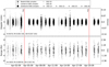 |
Fig. 1. Residuals of two-way Doppler data at 60 s count-time (top) and range data at 300 s (bottom) for a typical arc. The different colours and markers specify the complex and specific Deep Space Station (DSS) used for each tracking pass. The red vertical lines indicate the two flybys of Titan performed within the analysed period. In the bottom left boxes, the amount, mean, and standard deviation of residuals are reported. |
2.2. Set-up
In order to reconstruct the orbit, we divided the trajectory in arcs that span two consecutive flybys. This approach was also followed by the navigation team (Bellerose et al. 2016). The extension of these arcs is mainly limited by the dynamical model accuracy in predicting the outbound trajectory of the satellite encounter. The resulting arc subdivision provides for an overlap between two consecutive flybys (e.g. if the i-th arc includes T52 and T53 as in Fig. 1, the (i+1)-th arc includes T53 and T54); this allows for a more robust estimate of the orbit and permits, for each flyby, to choose the arc that provides the most accurate solution.
In our OD solution, using navigation reconstructions (Antreasian et al. 2005, 2007, 2008; Pelletier et al. 2012; Bellerose et al. 2016) as a priori information, we then solved for the spacecraft initial conditions, corrections to OTMs direction and amplitude, small forces ΔV components, RTG acceleration, a scale factor for SRP, and stochastic accelerations. The latter are used for compensating remaining mis-modellings in the spacecraft dynamics; in particular, constant accelerations to the level of 5 × 10⁻¹³ km s−2 for each spacecraft-fixed frame axis are estimated and updated every eight hours. Moreover, during closer Titan flybys, we account for drag coefficients and corrections to the predicted RCS thrusts, which are used to counter the atmospheric torques and maintain the desired attitude.
A representation of the magnitude of the main accelerations acting on the spacecraft during a typical low-altitude flyby of Titan is given in Fig. 2. The plot shows the relevance of non-gravitational (NG) accelerations in the evolution of the trajectory and how their correct modelling plays a decisive role in obtaining a good reconstruction of the orbit. Because of the limited knowledge of such forces, in some passes additional stochastic accelerations to the level of 5 × 10⁻⁹ km s−2 along the spacecraft Z-axis2 and 5 × 10⁻¹¹ km s−2 on X and Y were estimated and updated every five minutes. We extracted the gravities of Titan and Saturn, which still introduce a major effect on the spacecraft dynamics, from Durante et al. (2019) and Iess et al. (2019) and these values were not adjusted in our fit.
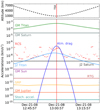 |
Fig. 2. Main accelerations acting on the spacecraft (bottom panel) in a close flyby of Titan (here represented for T50), during which Cassini flew over the moon at an altitude of 960 km (as shown in the top panel). |
The orbits and point-mass gravity accelerations from the other solar system planets were computed using INPOP17a planetary ephemerides (Viswanathan et al. 2017), while gravity interactions with the other satellites of Saturn were derived from Jet Propulsion Laboratory’s (JPL) SAT389 (Jacobson 2016a) and SAT393 (Jacobson 2016b). For the ephemerides of Titan we used the solution provided by the navigation team (Antreasian et al. 2005, 2007, 2008; Pelletier et al. 2012; Bellerose et al. 2016). The reconstruction of Titan orbit by the navigation team is sufficiently accurate (Boone & Bellerose 2017) to obtain a good fit of the data (see Fig. 1) except for the arcs of 2006, which were reconstructed in an early phase of the mission when limited knowledge of the Saturnian system afflicted the navigation reconstruction. For those arcs requiring further adjustments, we estimated minor3 corrections to Titan state, of the order of tens of metres. An assessment of the impact of the uncertainty of Titan ephemeris on orbit reconstruction is provided in Boone & Bellerose (2017).
Although we used largely de-weighted, range measurements in our analysis; those are affected by potential biases from path delays introduced by the propagation media (e.g. troposphere, ionosphere, and solar plasma), instrumentation at the ground station, and the spacecraft radio system. Before (pre-cal) or after (post-cal) each pass, the ground station provides a characterisation of the station delay with metres-level uncertainty (Border & Paik 2009). During the pass, negligible variations of about 10 cm, below the RMS level of the observables (see Fig. 1), are expected. Water-vapour radiometer (only for gravity-dedicated passes) and Global Positioning System (GPS) calibrations are available for media delays. However, to compensate for the remaining calibration error, we estimated a common bias on the range observables per tracking pass. These biases were modelled as stochastic parameters, updated every 24 h, with large a priori uncertainty (500 RU) in absorbing both the calibration residual and the planetary ephemerides mis-modelling. Errors in the relative location of Saturn and Earth cause an erroneous positioning of Cassini with respect to the ground station, and thus a miscalculation of the range computed observable. In our fit we did not correct for this term, but we absorbed it with the range biases.
The estimated values are reported in Fig. 3. A significant signature with an annual frequency and an amplitude of about 50 m is present as a result of the use of INPOP17a. Thanks to the enhanced accuracy of the new points, it is now possible to improve this ephemeris. A fundamental advantage of our analysis with respect to Hees et al. (2014) is derived from the choice of processing longer arcs that include moon flybys and OTMs. In this way, it is possible to better constrain the position of Cassini with a continuous orbit (see Fig. 3) and, therefore, to produce more accurate normal points for Saturn ephemeris. The analysis has been performed using JPL’s Mission Analysis, Operations, and Navigation Toolkit Environment (MONTE) for both integrating the equations of motion and generating the computed observables with its observation model (Moyer 2005).
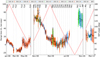 |
Fig. 3. Estimated range biases (one per pass) and associated formal uncertainties for the three analysed periods. A clear signal is introduced by Earth and Saturn ephemerides (INPOP17a). The scatter, instead, is related to the station delays calibration errors. The red line shows the relative SEP angle. |
2.3. Production of normal points
Once we dispose of a new reconstructed trajectory for Cassini and refined corrections to Saturn ephemeris in the form of range biases, we can proceed with the construction of the normal points. These are virtual measurements time-tagged in the middle of each tracking pass, providing the signal round-trip light-time between the ground-station and the spacecraft, corrected for the Earth’s troposphere and ionosphere delays and the relative range bias, properly transformed in time delay. The associated uncertainty is given by the estimated range bias covariance yielded from OD. A representation of the formal uncertainty levels are given by the error bars shown in Fig. 3.
The signal propagation time is computed as
 (2)
(2)
 (3)
(3)
where tr and tt are the times at receiver and transmitter, respectively, rr(tr) and rt(tt) are the positions of the receiver and transmitter in the inertial frame at the receiving and transmitting time, and ΔGR is the general relativity correction term (Moyer 2005). The solution, which requires an iterative process to account for the relative motion of the bodies within the propagation time, is performed using MONTE utilities.
Therefore, the normal point is given by
 (4)
(4)
where (⋅)uplink and ( ⋅ )dnlink terms represent the uplink and downlink propagation times, δstn the possible station delays, and ρbias the estimated range bias expressed in seconds.
3. Grand Finale and Titan gravity flybys
Additional points were produced based on the OD solutions of the Grand Finale passes (Iess et al. 2019) and Titan flybys (Durante et al. 2019) dedicated to gravity.
3.1. Grand Finale
During Grand Finale orbits performed at the end of its mission, Cassini flew close to Saturn as it never did before, passing in between the rings and the upper clouds of the planet. Five pericentres of these 22 orbits were devoted to measuring the gravity field and rings mass of Saturn. Exploiting the exquisite orbit reconstruction obtained within these passes, characterised by a metre-level uncertainty with respect to the planet at the closest approach (C/A), we have produced nine normal points with an unprecedented accuracy of ∼3 m. These data allowed us to extend Cassini dataset until the end of the mission in 2017.
3.2. Titan gravity flybys (TGF)
Of the 127 close encounters Cassini made with Titan in 13 years, 9 were dedicated to gravity measurements (plus an additional flyby primarily devoted to imaging the moon’s north polar lakes). During these flybys, the Cassini HGA antenna pointed towards Earth and no manoeuvres were executed for few days before and after the flyby to grant the maximum dynamical stability to the platform. Moreover, the altitude, ranging from 2397 and 3651 km, was chosen to avoid disturbances from the moon’s thick atmosphere (see Sect. 2). This allowed Durante et al. (2019) to reconstruct the spacecraft trajectory with higher accuracy compared to that attainable in the other flybys. For each gravity flyby, four to five measurements were produced (one per tracking pass) for a total of new 42 normal points. The average uncertainty of these measurements is ∼7.4 m; the C/A points, which were constrained by Titan’s gravity, exhibit the highest accuracies.
4. INPOP planetary ephemerides
Since 2003 INPOP planetary ephemerides have been built by numerically integrating the equations of motion of the eight planets of our solar system, plus Pluto and the Moon, with accurate modelling of the Moon’s libration and the Earth’s rotation. Their initial conditions at J2000 are estimated using a weighted least-squares filter on the most accurate measurements available, derived from tracking data of interplanetary missions around the solar system, but also ground-based optical observations and Lunar laser ranging measurements (Fienga et al. 2019; Viswanathan et al. 2018).
4.1. Data sample
As described in Fienga et al. (2019), 2016b), the latest INPOP version, INPOP19a, benefits from several improvements in the field of the solar plasma correction and the determination of asteroid masses (Fienga et al. 2019). In Fienga et al. (2019), the use of Monte Carlo least squares with a priori information on the asteroid spectra leads to significant improvement in the constraints of the asteroid masses and in the post-fit residuals (see Table 1). In particular, with INPOP19a we estimated the masses of 343 objects of the main belt. The addition of the new normal points for the Jovian barycentre, obtained with the gravity science experiment of the Juno mission (Iess et al. 2018), and the new adjustment of the Moon orbit and rotation (Fienga et al. 2016b) should be also noted. Another major input is derived from the use of the normal points for the Saturn system barycentre deduced from the analysis of Cassini tracking data described in Sect. 2 and from OD solutions of the gravity Grand Finale passes and Titan flybys (see Sect. 3).
Datasets included in INPOP19a fit.
The INPOP19a full dataset is presented in Table 1, along with a comparison of the weighted RMS (WRMS) of the post-fit residuals obtained with INPOP19a and INPOP17a. Beside the aforementioned points, the Cassini dataset includes ten Very Long Baseline Interferometry (VLBI) measurements and 165 normal points deduced by the JPL Doppler-only analysis described in Hees et al. (2014). The time span of these observations is from 2004 to 2014, with an estimated RMS of 25 m. The augmented dataset for Saturn required some modifications in the INPOP dynamical modelling of the outer solar system for fitting together the three Cassini data samples previously described.
4.2. Update in the Kuiper belt modelling
Firstly, to update our representation of the solar system with the most recent estimates, we added the most massive TNOs to the list of planetary perturbers to INPOP19a (see Table 2). Along with the main belt asteroids, the orbits of these TNOs are integrated together with those of the planets. We fixed the masses of these objects, since they all have at least one natural satellite, and their masses are thus very accurately measured by studying their moon orbits. Secondly, a ring representing the average influence of TNOs enclosed in the two main resonances with Neptune (3:2 and 2:1) was modelled in INPOP19a. To do so, we introduce the accelerations induced by point-mass bodies spread over three circular, not inclined orbits located at 39.4, 44.0, and 47.5 AU, to which we attribute one-sixth, two-thirds, and one-sixth of the total mass, respectively (the same configuration adopted by Pitjeva & Pitjev 2018). The ring at 44.0 AU has more mass, as it represents the sum of the two populations of objects, the resonant and classical Kuiper belt objects (KBOs), with semi-major axes between 39.4 and 47.5 AU. The total mass is then estimated in the INPOP adjustment. The high correlations (98.5%) between the masses of each ring lead to an impossible estimation of the separate contributions.
Masses of the TNOs individually included in INPOP19a set-up.
With the INPOP19a extended dataset (Table 1), which now includes the Juno and Cassini data, we obtain for the TNOs ring a mass of
 (5)
(5)
4.3. Comparison with INPOP17a
Beside providing an overview on INPOP dataset, Table 1 also shows the improvements brought by the refined INPOP19a dynamical model over previous INPOP delivery, INPOP17a, in terms of WRMS residuals. Some noticeable enhancements are registered for Mars data thanks to the new asteroid masses estimate (see Sect. 4.1), for the newly added normal points from Juno gravity pericentres and, especially, for Saturn.
In particular, the effect of the new modelling on Cassini data is clearly visible in the residuals shown in Fig. 4 and in Table 3, where the WRMS values of Cassini datasets for the different models previously described are reported. In Fig. 4, the post-fit residuals of the normal points deduced from the Cassini mission are depicted for INPOP17a (where no TNOs are included either individually or by a ring) and three other solutions: one including the individual perturbations of the most massive TNOs (see Table 2), but without the TNO ring model; a second without the individual TNOs, but with the ring and; the last representing INPOP19a solution, which features both the ring and the TNOs. It evidently appears that the combined use of the individual TNOs together with the adjustment of the mass of a TNO ring significantly improves the post-fit residuals, in particular if we consider an interval of time spread over several decades. In INPOP17a, the TNO accelerations were not required since the time span of the Cassini data was limited to almost 10 years (from 2004 to 2014) and with lower accuracies (∼25 m for JPL data). With the addition of Grand Finale points, the data sample has been extended over 13 years (the full duration of Cassini mission), and INPOP17a model is not able to reproduce the data anymore, showing strong signatures in the residuals, including a bias on the latest period (Grand Finale points). Such a trend is not present when we include the modelling which accounts for both the individual TNOs and the ring.
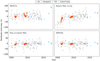 |
Fig. 4. Saturn post-fit residuals for the four Cassini datasets. These include the residuals obtained with INPOP17a, where no modelling of TNOs is included (top left); a solution accounting for the individual perturbations of the 9 most massive TNOs (top right); a solution including the TNO ring but none of the massive TNOs (bottom left); and INPOP19a, which includes both the ring model and the individual TNOs. The different colours indicate the 4 range datasets as presented in Table 1. |
Cassini data WRMS values for multiple INPOP solutions.
5. Discussion
5.1. Importance of the different Cassini datasets
Figure 4 also offers a qualitative idea of the sensitivity of the different datasets to the trans-Neptunian solar system modelling. In particular, the top left plot shows the scarce sensitivity of JPL points; a proper fit of these data is achievable without introducing any TNO perturbation, as we obtained with INPOP17a. An evidence of this aspect is also given in Table 3, where the limited variation registered on the WRMS of these data from INPOP17a and INPOP19a (from 1.1 to 0.99) is reported.
On the contrary, Grand Finale points exhibit the highest sensitivity because of their unique time frame and peculiar geometry perspective. The WRMS in this case shows a significant improvement, from a value of ∼30 for INPOP17a and close to unity for INPOP19a. Most of the enhancement derives from the introduction of the TNO ring in the dynamical model and the estimate of its mass; however, the contribution of the massive TNOs results to be significant for the early navigation data (Feb.-Jul. 2006) and for the Grand Finale measurements, providing a reduction of the residuals’ WRMS from 2.58 to 1.14.
Finally, TGF data showed a dispersion of the residuals larger than their expected accuracy (see Sect. 3.2). This can be explained by the fact that they are significantly less than the navigation data (42 vs. 572), sharing overall the same accuracy. Moreover, the navigation points are mostly concentrated in a limited interval of time (2008–2009), which leads the filter to produce a better fit of these data to the detriment of TGF residuals, which are distributed on a larger interval. However, the contribution of this dataset to our estimate of the Kuiper belt mass is limited. We performed a test by removing these data from the fit, obtaining a solution that is compatible with the original result.
5.2. Comparison with previous analyses
Two types of analyses have hitherto been published: those based on KBO direct observations and those deduced from the KBO perturbations on planetary ephemerides. In Bernstein et al. (2004), based on Hubble Space Telescope observations, the authors deduced a distribution of sizes and infer surface density values, finding a mass of the Kuiper belt of about 0.010 M⊕ when considering only KBOs with inclination smaller than 5°. If we add their estimations of excited KBOs (objects with inclination greater than 5°), the total mass deduced from Bernstein et al. (2004) becomes 0.018 M⊕. The value is low compared to our estimate, but also in comparison with the Gladman et al. (2001) results. In the latter work, the authors used a different assumption for the size distribution, leading to an estimation of the mass of the total Kuiper belt in between 0.04 and 0.1 M⊕. This interval of masses nicely frames our result, which was obtained completely independently.
The perturbations of KBOs on the planetary orbits were considered in Pitjeva & Pitjev (2018). Two models of the ring perturbations were used: one numerical model that is similar to our approach (exposed in Sect. 4.2) and one analytical approach; both of these models give consistent results. The analysis by these authors does not include the Cassini normal points produced within our work, but it is based, for Cassini range, on Hees et al. (2014) data alone. Therefore, if we limit the data sample to that used by Pitjeva & Pitjev (2018), we obtain a mass of
 (6)
(6)
which is consistent at 3σ with their value,  . It is worth noting that the masses of the major TNOs included in our model (see Table 2) are fixed in INPOP adjustment, while 31 TNO masses are fitted in Pitjeva & Pitjev (2018). It is possible that part of TNO masses in INPOP are absorbed by the TNO ring mass, inducing a slightly bigger value than that obtained by Pitjeva & Pitjev (2018). If we add the masses of the fixed TNOs to the mass of the ring, the differences decrease as we obtain
 (7)
(7)
which is then compatible at 2σ with the estimated value of Pitjeva & Pitjev (2018),  .
.
Although it is useful to assess the two results, the sum of masses (Mtotal = Mring + MTNOs) does not provide a complete comparison of our estimate and the result by Pitjeva & Pitjev (2018); this is because of the different mass distribution considered in the two models, and the degeneracy between the mass of the ring and its distance to the solar system barycentre. Finally, the mass found in this paper, as well as the masses previously discussed, are consistent with the Kuiper belt mass obtained from simulated populations, such as Levison et al. (2008).
6. Conclusions
We have presented an efficient method for producing normal points for the construction of planetary ephemerides; we also provide the associated uncertainties. A total of 572 points were produced from Cassini navigation data; these have an average accuracy of 6 m, 42 points from Titan gravity flybys, and 9 from Grand Finale pericentres.
By adding these points to the INPOP planetary ephemerides dataset (see Table 1) we built INPOP19a, which includes new modelling of TNOs that is necessary to fit the new normal points for Saturn system barycentre produced in this work (see Fig. 4). In particular nine massive TNOs have been added to the list of integrated bodies along with a series of three rings representing the KBOs in the 2:1 and 3:2 resonances with Neptune. We fit the total mass of the rings and provide an estimate of (0.061 ± 0.001)M⊕, which is compatible with previous analyses and in line with theoretical predictions.
The flyby labelling provides for the initial of the interested moon (e.g. T for Titan, E for Enceladus) followed by the encounter number.
Z-axis corresponds to the HGA pointing axis.
Negligible in terms of induced shift on the Saturn system barycentre considering the range data accuracy.
Acknowledgments
The authors would like to thank their colleagues of the Sapienza Radio Science, GéoAzur and IMCCE laboratories for the fruitful discussions. This work has been partially funded by the Italian Space Agency (ASI) under the contract 2017-10-H.0, the CNRS, the UCA Academie 3 and the French Space Agency (CNES). This work was also supported by the Programme National GRAM of CNRS/INSU with INP and IN2P3 co-funded by CNES.
References
- Antreasian, P., Bordi, J. J., Criddle, K., et al. 2005, AAS/AIAA Astrodynamics Specialist Conf., Lake Tahoe, CA, AAS 05–312 [Google Scholar]
- Antreasian, P., Bordi, J. J., Criddle, K., et al. 2007, AAS/AIAA Astrodynamics Specialist Conf., Mackinac Island, MI, AAS 07-000 [Google Scholar]
- Antreasian, P., Ardalan, S., Bordi, J., et al. 2008, SpaceOps Conf., Heidelberg, Germany, AIAA 2008-3433 [Google Scholar]
- Asmar, S. W., Armstrong, J. W., Iess, L., & Tortora, P. 2005, Radio Sci., 40, RS2001 [CrossRef] [Google Scholar]
- Batygin, K., & Brown, M. E. 2016, AJ, 151, 22 [NASA ADS] [CrossRef] [Google Scholar]
- Batygin, K., Adams, F. C., Brown, M. E., & Becker, J. C. 2019, Phys. Rep., 805, 1 [NASA ADS] [CrossRef] [Google Scholar]
- Becker, J., Prasanna, V. K., Weimer, M., et al. 2018, 2018 IEEE Int. Parallel. Distrib. Process. Symp. Workshops (IPDPSW), 81 [CrossRef] [Google Scholar]
- Bellerose, J., Nandi, S., Roth, D., et al. 2016, AAS 16–142 [Google Scholar]
- Bernstein, G. M., Trilling, D. E., Allen, R. L., et al. 2004, AJ, 128, 1364 [NASA ADS] [CrossRef] [Google Scholar]
- Bierman, G. J. 1977, Factorization Methods for Discrete Sequential Estimation, 128 [Google Scholar]
- Boone, D., & Bellerose, J. 2017, ISSFD 2017 [Google Scholar]
- Border, J. S., & Paik, M. 2009, Interplanetary Net. Prog. Rep., 42, 1 [Google Scholar]
- Brown, M. E., Trujillo, C., & Rabinowitz, D. 2004, ApJ, 617, 645 [NASA ADS] [CrossRef] [Google Scholar]
- Brown, T. S. 2018, AIAA 2018–2023 [Google Scholar]
- Durante, D., Hemingway, D. J., Racioppa, P., Iess, L., & Stevenson, D. J. 2019, Icarus, 326, 123 [CrossRef] [Google Scholar]
- Fienga, A., Laskar, J., Manche, H., & Gastineau, M. 2016a, A&A, 587, L8 [NASA ADS] [CrossRef] [EDP Sciences] [Google Scholar]
- Fienga, A., Laskar, J., Manche, H., & Gastineau, M. 2016b, ArXiv e-prints [arXiv:1601.00947] [Google Scholar]
- Fienga, A., Avdellidou, C., & Hanuš, J. 2019, MNRAS, 492, 589 [Google Scholar]
- Fienga, A., Di Ruscio, A., Bernus, L., et al. 2020, A&A, 640, A6 [CrossRef] [EDP Sciences] [Google Scholar]
- Folkner, W., Jacobson, R. A., Park, R., & Williams, J. G. 2016, AAS/DPS Meet. Abstracts, 48, 120.07 [Google Scholar]
- Gladman, B., Kavelaars, J. J., Petit, J.-M., et al. 2001, AJ, 122, 1051 [NASA ADS] [CrossRef] [Google Scholar]
- Hees, A., Folkner, W. M., Jacobson, R. A., & Park, R. S. 2014, Phys. Rev. D, 89, 102002 [NASA ADS] [CrossRef] [Google Scholar]
- Holman, M. J., & Payne, M. J. 2016a, AJ, 152, 80 [NASA ADS] [CrossRef] [Google Scholar]
- Holman, M. J., & Payne, M. J. 2016b, AJ, 152, 94 [NASA ADS] [CrossRef] [Google Scholar]
- Iess, L., Stevenson, D. J., Parisi, M., et al. 2014a, Science, 344, 78 [NASA ADS] [CrossRef] [Google Scholar]
- Iess, L., Di Benedetto, M., James, N., et al. 2014b, Acta Astronaut., 94, 699 [CrossRef] [Google Scholar]
- Iess, L., Folkner, W. M., & Durante, D. 2018, Nature, 555, 220 [NASA ADS] [CrossRef] [Google Scholar]
- Iess, L., Militzer, B., Kaspi, Y., et al. 2019, Science, 364, aat2965 [NASA ADS] [CrossRef] [Google Scholar]
- Jacobson, R. A. 2016a, Satellite Ephemeris File Release: SAT389 [Google Scholar]
- Jacobson, R. A. 2016b, Satellite Ephemeris File Release: SAT383 [Google Scholar]
- Jewitt, D., & Luu, J. 1993, Nature, 362, 730 [NASA ADS] [CrossRef] [Google Scholar]
- Lee, A. Y., & Burk, T. A. 2019, J. Spacecraft Rockets, 56, 158 [CrossRef] [Google Scholar]
- Levison, H. F., Morbidelli, A., Van Laerhoven, C., Gomes, R., & Tsiganis, K. 2008, Icarus, 196, 258 [NASA ADS] [CrossRef] [Google Scholar]
- Moyer, T. 2005, Formulation for Observed and Computed Values of Deep Space Network Data Types for Navigation (John Wiley & Sons Ltd.) [Google Scholar]
- Pelletier, F., Antreasian, P., Bordi, J., et al. 2006, AAS 06–141 [Google Scholar]
- Pelletier, F., Antreasian, P., Ardalan, S., et al. 2012, SpaceOps 2012 Conf., Stockholm, Sweden [Google Scholar]
- Pitjeva, E. V., & Pitjev, N. P. 2018, Celestial Mech. Dyn. Astron., 130, 57 [Google Scholar]
- Prialnik, D., Barucci, M., & Young, L. 2020, The Trans-Neptunian Solar System (Elsevier) [Google Scholar]
- Roth, D., Hahn, Y., Owen, B., & Wagner, S. 2018, 2018 SpaceOps Conf., AIAA 2018-2647 [Google Scholar]
- Standish, E. M. J. 1990, A&A, 233, 252 [Google Scholar]
- Tapley, B. D., Schutz, B. E., & Born, G. H. 2004, Statistical Orbit Determination (United States: Elsevier Inc.) [Google Scholar]
- Thornton, C. L., & Border, J. S. 2000, in Radiometric Tracking Techniques for Deep-Space Navigation (Jet Propulsion Laboratory), Deep-space Navigation Commun. Ser., 1 [Google Scholar]
- Trujillo, C. A., & Sheppard, S. S. 2014, Nature, 507, 471 [NASA ADS] [CrossRef] [Google Scholar]
- Viswanathan, V., Fienga, A., Gastineau, M., & Laskar, J. 2017, INPOP17a Planetary Ephemerides [Google Scholar]
- Viswanathan, V., Fienga, A., Minazzoli, O., et al. 2018, MNRAS, 476, 1877 [NASA ADS] [CrossRef] [Google Scholar]
All Tables
All Figures
|
Fig. 1. Residuals of two-way Doppler data at 60 s count-time (top) and range data at 300 s (bottom) for a typical arc. The different colours and markers specify the complex and specific Deep Space Station (DSS) used for each tracking pass. The red vertical lines indicate the two flybys of Titan performed within the analysed period. In the bottom left boxes, the amount, mean, and standard deviation of residuals are reported. |
| In the text | |
|
Fig. 2. Main accelerations acting on the spacecraft (bottom panel) in a close flyby of Titan (here represented for T50), during which Cassini flew over the moon at an altitude of 960 km (as shown in the top panel). |
| In the text | |
|
Fig. 3. Estimated range biases (one per pass) and associated formal uncertainties for the three analysed periods. A clear signal is introduced by Earth and Saturn ephemerides (INPOP17a). The scatter, instead, is related to the station delays calibration errors. The red line shows the relative SEP angle. |
| In the text | |
|
Fig. 4. Saturn post-fit residuals for the four Cassini datasets. These include the residuals obtained with INPOP17a, where no modelling of TNOs is included (top left); a solution accounting for the individual perturbations of the 9 most massive TNOs (top right); a solution including the TNO ring but none of the massive TNOs (bottom left); and INPOP19a, which includes both the ring model and the individual TNOs. The different colours indicate the 4 range datasets as presented in Table 1. |
| In the text | |
Current usage metrics show cumulative count of Article Views (full-text article views including HTML views, PDF and ePub downloads, according to the available data) and Abstracts Views on Vision4Press platform.
Data correspond to usage on the plateform after 2015. The current usage metrics is available 48-96 hours after online publication and is updated daily on week days.
Initial download of the metrics may take a while.