| Issue |
A&A
Volume 638, June 2020
|
|
|---|---|---|
| Article Number | L11 | |
| Number of page(s) | 5 | |
| Section | Letters to the Editor | |
| DOI | https://doi.org/10.1051/0004-6361/202038373 | |
| Published online | 23 June 2020 | |
Letter to the Editor
Nature versus nurture: relic nature and environment of the most massive passive galaxies at z < 0.5
1
INAF – Osservatorio Astrofisico di Arcetri, Largo Enrico Fermi 5, 50125 Firenze, Italy
e-mail: crescenzo.tortora@inaf.it
2
School of Physics and Astronomy, Sun Yat-sen University Zhuhai Campus, Daxue Road 2, 519082 Tangjia, Zhuhai, Guangdong, PR China
3
INAF – Osservatorio Astronomico di Capodimonte, Salita Moiariello 16, 80131 Napoli, Italy
4
INAF – Osservatorio Astronomico di Padova, Vicolo Osservatorio 5, 35122 Padova, Italy
5
Department of Physics, University of Oxford, Keble Road, Oxford OX1 3RH, UK
6
Dipartimento di Fisica e Astronomia – Alma Mater Studiorum Università di Bologna, Via Piero Gobetti 93/2, 40129 Bologna, Italy
7
INAF – Osservatorio di Astrofisica e Scienza dello Spazio di Bologna, Via Piero Gobetti 93/3, 40129 Bologna, Italy
8
INFN – Sezione di Bologna, Viale Berti-Pichat 6/2, 40127 Bologna, Italy
9
Argelander-Institut für Astronomie, Auf dem Hügel 71, 53121 Bonn, Germany
10
Dipartimento di Scienze Fisiche, Università di Napoli Federico II, Compl. Univ. Monte S. Angelo, 80126 Napoli, Italy
11
Instituto de Astrofísica Pontificia Universidad Católica de Chile, Avenida Vicuña Mackenna, 4860 Santiago, Chile
12
Zentrum für Astronomie, Universitatät Heidelberg, Philosophenweg 12, 69120 Heidelberg, Germany
13
Institut für Theoretische Physik, Ruprecht-Karls-Universität Heidelberg, Philosophenweg 16, 69120 Heidelberg, Germany
Received:
7
May
2020
Accepted:
4
June
2020
Relic galaxies are thought to be the progenitors of high-redshift red nuggets that for some reason missed the channels of size growth and evolved passively and undisturbed since the first star formation burst (at z > 2). These local ultracompact old galaxies are unique laboratories for studying the star formation processes at high redshift and thus the early stage of galaxy formation scenarios. Counterintuitively, theoretical and observational studies indicate that relics are more common in denser environments, where merging events predominate. To verify this scenario, we compared the number counts of a sample of ultracompact massive galaxies (UCMGS) selected within the third data release of the Kilo Degree Survey, that is, systems with sizes Re < 1.5 kpc and stellar masses M⋆ > 8 × 10¹⁰ M⊙, with the number counts of galaxies with the same masses but normal sizes in field and cluster environments. Based on their optical and near-infrared colors, these UCMGS are likely to be mainly old, and hence representative of the relic population. We find that both UCMGS and normal-size galaxies are more abundant in clusters and their relative fraction depends only mildly on the global environment, with denser environments penalizing the survival of relics. Hence, UCMGS (and likely relics overall) are not special because of the environment effect on their nurture, but rather they are just a product of the stochasticity of the merging processes regardless of the global environment in which they live.
Key words: galaxies: evolution / galaxies: formation / galaxies: abundances
© ESO 2020
1. Introduction
According to the current understanding of galaxy formation, cosmic structures are formed in a hierarchical fashion. At the very early stages of the universe history, gas condenses within the primordial dark matter perturbations (Blumenthal et al. 1984; Springel et al. 2005), forming the first stars and thus the first galaxies. With time, these objects grow through mergers, generating increasingly larger galaxies, and experience physical transformations influenced by the wide range of environments that they live in (Daddi et al. 2005; Trujillo et al. 2007). Determining the role of internal processes and environment (this last including mergers), which astronomers refer to as the “nature versus nurture” problem (e.g., Irwin 1995), is crucial for understanding the formation and evolution of galaxies.
Recent studies seem to suggest that the most massive and passive galaxies with M⋆ ≳ 5 × 10¹⁰ M⊙ are formed through a two-phase formation scenario (Oser et al. 2010). During the first phase, an intense and quick burst of star formation at z > 2 forms the bulk of the central mass and after the star formation quenches, generates compact massive quiescent galaxies (red nuggets). Then, during a more extended second phase, mergers and gas inflows cause a dramatic size growth despite a very slight change in mass (e.g., Hilz et al. 2013; Tortora et al. 2014). Red nuggets, which are about four times smaller than local massive galaxies, are very common at z > 2, but are expected to be rare in the local universe (van Dokkum et al. 2006; Cimatti et al. 2008; Bezanson et al. 2009). Because of the stochastic nature of mergers, simulations predict that only ∼1 − 10% of the red nuggets evolve undisturbed until the present cosmic epoch, with a very slight change in size, and therefore represent outliers of the local size-mass relation (Hopkins et al. 2009; Quilis & Trujillo 2013); these peculiar galaxies are named “relics”. The number of relics depends on the physical processes acting during the second phase, and in particular, on the relative contribution of major and minor galaxy mergers. Therefore, comparing relic abundance and properties with those of normal-size equally massive galaxies allows us to measure the merging effect. The stars that formed in red nuggets are thought to be the in situ populations living in the core of local giant ellipticals. However, this population is mixed with the accreted population that formed during mergers and inflows. With relics, which lack the accreted component, we can therefore probe the processes that shape the galaxy formation at high redshift with a precision that is only attainable for the nearby universe, in order to separate nature from nurture.
In the past few years, several different studies found and characterized compact massive galaxies and relics in local environments. The only difference between the former and the latter is the age of the stellar population, which for relics is as old as the universe. They extended the analysis up to z = 0.7, where the number counts are expected to be higher than in the local universe (e.g., Tortora et al. 2018a versus Ferré-Mateu et al. 2017) and high enough to study the evolution of these galaxies within different environments.
While the number of discovered compact galaxies is increasing at z ≲ 0.5 (e.g., Tortora et al. 2018a, and references therein), there is still an open debate about possible selection biases related to the environment. The results of large sky surveys such as the Sloan Digital Sky Survey (SDSS1) show a sharp decline in compact galaxy number density of more than three orders of magnitude below the high-redshift values (z ∼ 2; Trujillo et al. 2009; Taylor et al. 2010). In contrast, data in nearby clusters indicate a number density of two orders of magnitude above the SDSS one, which is comparable with the number density at high redshift (Valentinuzzi et al. 2010; Poggianti et al. 2013a,b).
Thus, the following questions need answers. Is cluster environment favoring the formation of relics? Are these rare systems descendants of red nuggets or formed preferentially in clusters from larger galaxies deprived of their outer stellar populations?
Using 271 compact, massive (M⋆ ≳ 1010 M⊙) and quiescent galaxies at 0.1 < z ≲ 0.6 in the COSMOS field, Damjanov et al. (2015a) have demonstrated that compact quiescent galaxies populate a similar range of environment as the parent population of equally massive quiescent galaxies. The numbers of these compact and normal-size systems are not yet statistically significant, however, for an investigation of the environmental dependence of the most massive, red, and extremely compact systems, that are the most likely direct descendants of high-z red nuggets.
In this Letter we make a crucial step forward in understanding the role of the environment in relic formation and evolution. As realistic markers of the relic population we use the largest available sample (∼1000 objects) of ultracompact massive galaxies (UCMGS hereafter), which are defined as the most compact (Re < 1.5 kpc) and most massive (M⋆ > 8 × 10¹⁰ M⊙) red galaxies at z < 0.5. These UCMGS have been found by Tortora et al. (2018a, hereafter T18) within the footprint of the VLT Survey Telescope (VST) Kilo Degree Survey (KiDS, de Jong et al. 2017). We investigate their number counts in terms of the environment (fields versus clusters) and compare our findings with a KiDS parent sample of normal-size massive galaxies. We adopt a cosmological model with (Ωm, ΩΛ, h) = (0.3, 0.7, 0.7), where h = H0/100 km s−1 Mpc−1 (Komatsu et al. 2011).
2. Galaxy samples
The galaxy selection started from the KiDS multiband source catalog that is included in the third KiDS Data Release (KiDS–DR3, de Jong et al. 2017). After masking of bad areas, we collected a catalog of about 5 million galaxies within an effective area of 333 sq. deg. The photometric catalog includes u-, g-, r-, and i-band magnitudes (de Jong et al. 2017), structural parameters obtained from the point spread function (PSF)-convolved fit of the Sérsic profile (Roy et al. 2018), photometric redshifts (Cavuoti et al. 2017), and stellar masses derived from spectral energy distribution (SED) fitting of single-burst (Bruzual & Charlot 2003) stellar population synthesis theoretical models (T18). We complemented these data with a galaxy classification based on SED fitting and VIKING J and K magnitudes, with which we set up a color cut in the g–J versus J–K plane to further remove stellar contaminants and very blue galaxies, as discussed in T18. Because most of our (compact and more extended) galaxies are elliptical, we expect that the number of galaxies that are misclassified as stars from the KiDS pipeline is very small. For more details about data extraction, quality checks, and sample selection, we refer to our previous papers (Roy et al. 2018; Tortora et al. 2016; T18; Scognamiglio et al. 2020, S20 hereafter).
Here, we only use galaxies with good surface photometry fits, selecting a cumulative r-band signal-to-noise ratio, S/N > 50, a good χ2 (< 1.5), and realistic structural parameters in g, r, and i bands (Sérsic index n > 0.5, axis ratios q > 0.1, and effective radius Θe > 0.05″); these criteria also reduce the contaminations by misclassified stars, disk-on galaxies, and systems with spiral arms.
We selected a sample of 104 383 massive galaxies with M⋆ > 8 × 10¹⁰ M⊙ at redshifts z < 0.5. According to their median effective radius Re, calculated as the median of the g-, r-, and i-band Re, we then classified them into two separate samples: normal-size massive galaxies (NSMGS), and ultracompact massive galaxies (UCMGS):
-
NSMGS: 103 388 objects with a median effective radius Re ≥ 1.5 kpc.
-
UCMGS: 995 objects with a median effective radius Re < 1.5 kpc instead.
The search for cluster candidates was made using the algorithm called Adaptive Matched Identifier of Clustered Objects (AMICO) (Bellagamba et al. 2018), which applies an optimal filter to select galaxy overdensities in a catalog with coordinates, photometric redshifts, and magnitudes of galaxies. We applied this algorithm to KiDS–DR3 (Bellagamba et al. 2019; Maturi et al. 2019; Radovich et al. 2020). Each galaxy is tagged with its distance from the cluster center and a membership probability, Pcl, that is, the probability (from 0 to 1) to be a cluster member. An estimate for the cluster virial radius (Rvir) is also available. In the following, we limit our analysis to galaxies with Pcl > 0.2.
3. Galaxy number counts and environment
In this section we discuss the numerical abundance of UCMGS and NSMGS, the fraction of UCMGS, and their distribution as a function of the environment. We then compare our results with literature and finally extend them to relic galaxies.
3.1. Number density calculation
Following T18, we started by determining number densities for NSMGS and UCMGS within the KiDS effective area, regardless of the environment. We binned galaxies according to redshift. As in T18, we optimized the redshift bins for the UCMG sample, setting a width of 0.1, except for the lowest-z bin that corresponds to the redshift interval (0.15 − 0.2); for NSMGS we also added the interval (0 − 0.15). We multiplied the number of candidates by farea = Asky/Asurvey, where Asky (=41 253 sq. deg.) is the full-sky area and Asurvey (=333 sq. deg.) is the effective KiDS area. The density was derived by dividing by the all-sky comoving volume corresponding to each redshift bin.
To obtain galaxy counts in clusters, we first selected cluster galaxies in each redshift bin, with Pcl > 0.2, within 1 Rvir, and we weighted them according to Pcl, giving more weight to galaxies that are more likely cluster members. For both NSMGS and UCMGS, the total number of galaxies in each redshift bin was then divided by the sum of the comoving volumes within Rvir of all the clusters and in that redshift bin.
Finally, we obtained the number of NSMGS or UCMGS in the fields by subtracting the cluster members from the total number of NSMGS or UCMGS. Similarly, the comoving volume was determined by subtracting the comoving volume occupied by clusters from the total volume. Clusters occupy a volume a factor ∼4 × 10⁻⁵ smaller than the whole effective volume we analyzed.
3.2. Number density and environment
In the left panel of Fig. 1 the number densities for field and cluster UCMGS are compared with those of NSMGS in the same environments. Number counts for field UCMGS are found to decrease with cosmic time from ∼9 × 10⁻⁶ Mpc−3 at z ∼ 0.5 to ∼10−6 Mpc−3 at z ∼ 0.15. This corresponds to a decrease of about nine times in about 3 Gyr (T18; S20). We found that UCMGS within 1 Rvir of the clusters are more abundant than field UCMGS with numbers counts of ∼5.7 × 10⁻³ Mpc−3 at z ≳ 0.25. The trend with redshift seems to be similar to the trend in the field, but we did not find any UCMGS in clusters below z = 0.25.
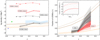 |
Fig. 1. Left panel: number density of UCMGS (solid line, squared points) and NSMGS (dashed lines, triangles) as a function of redshift and environment (black lines for field and red for cluster galaxies). Shaded regions correspond to 1σ errors, accounting for Poisson noise, cosmic variance, and uncertainties in size and mass selection, but neglecting the nominal uncertainties on the photometric redshifts (S20). The cyan line refers to number densities for UCMGS in the COSMOS area by Damjanov et al. (2015b). The green point and blue triangle are the results for compact galaxies from Poggianti et al. (2013a) and Ferré-Mateu et al. (2017), respectively. Orange and brown curves are extracted from Quilis & Trujillo (2013): dashed and solid lines refer to Guo et al. (2011, 2013) SAMs, respectively, while orange (brown) lines are for galaxies that have increased their mass by less than 10 (30)%. No selection in environment is performed in such simulations. Right panel: fraction of UCMGS, calculated with respect to the total parent population in fields (black) and clusters (red), as a function of redshift. Dark (light) shaded regions show 1σ (2σ) errors in each redshift bin. Dashed black and red lines are for UCMGS with log M⋆/M⊙ ≤ 11.2 dex in field and clusters, respectively. The Guo et al. (2011, 2013) results are also plotted. Inset: fraction of UCMGS in clusters as a function of the distance R from the center in units of Rvir. The dashed line is for UCMGS with log M⋆/M⊙ ≤ 11.2 dex. |
In the same plot, we also show the number counts for NSMGS in fields and clusters. The number counts are systematically larger than those of UCMGS in the same environment. The number counts of NSMGS are constant with redshift in clusters (∼1.5 Mpc−3) and in the field (∼4 × 10⁻⁴ Mpc−3). This suggests that the fraction of recently formed massive red galaxies is negligible. This is consistently with previous results (e.g., Cassata et al. 2013).
We also compared the results for UCMGS with independent findings. The cyan region in the left panel of Fig. 1 shows number densities of galaxies in the COSMOS survey (Damjanov et al. 2015b). Our results for field UCMGS (or equivalently, those determined from the whole survey area) are consistent with COSMOS number counts in the highest redshift bin, but are systematically lower at lower z, with differences of about one order of magnitude in the lowest-z bin. Below z ∼ 0.2, our number counts decrease by one order of magnitude and appear to follow the direction of the local estimate from Ferré-Mateu et al. (2017), who found a number density of ∼2 × 10⁻⁷ Mpc−3 within a sphere of radius 106 Mpc from us. Instead, over an area of 38 sq. deg., biased toward dense cluster environments, Poggianti et al. (2013a) have found four galaxies (older than 8 Gyr) that fulfill our criteria, corresponding to a large number density of ∼10−5 Mpc−3. KiDS number densities in cluster environments are three orders of magnitude larger than their values. The source of this large discrepancy is related to a different strategy used to normalize the number counts (our cluster volumes versus their volume calculated within the area of 38 sq. deg.). We finally compared our results with the density of compact galaxies extracted from semi-analytical models (SAMs) based on Millennium N-body simulations (Guo et al. 2011, 2013). There is a clear overlap with number density of field UCMGS.
3.3. Fraction of UCMGS and environment
We report here the total absolute numbers (weighted according to Pcl) of NSMGS and UCMGS in clusters and their fraction with respect to the total galaxy population (including field and cluster systems). The number of NSMGS in clusters is ∼22 246, which corresponds to ∼22% of the total number of NSMGS. Instead, the number of cluster UCMGS is ∼135, which is ∼14% of the total number of UCMGS. This trend is made more robust when we separate NSMGS into four Re bins (1.5 − 3), (3 − 5), (5 − 7), and (7 − 50) kpc. This shows that galaxies in clusters are 18, 19, 19, and 24% of the total in these Re bin, respectively. The tendency for higher mass galaxies to be preferentially found in clusters is therefore clear. The tendency is expected when we consider that higher density regions favor mergers, and thus the formation of larger galaxies.
The average size of the galaxies is only slightly larger in clusters (∼5% more). It reaches an increment of ∼11% at M⋆ > 2 × 10¹¹ M⊙, in agreement with the negligible or mild dependence found at low and intermediate redshift (Huertas-Company et al. 2013a,b; Lani et al. 2013).
In the right panel of Fig. 1 we plot the fraction of UCMGS with respect to the total galaxy population (including both NSMGS and UCMGS) in fields and clusters as a function of redshift. The left panel of the same figure shows that the fraction of UCMGS decreases in the last 3 Gyr, which is expected when we consider that the probabilitly of merging increases with time. The fraction of compact systems in clusters is smaller than that of the same galaxies in the field, and it is consistent within the typical uncertainties. As mergers are more likely to occur in clusters, the fraction of UCMGS that merge to form NSMGS is larger. These results clearly show that UCMGS are more abundant in clusters because the parent sample of massive galaxies is more abundant there, and not because of their compactness. Mirroring the comparison made in terms of number counts, the two sets of simulations in Quilis & Trujillo (2013) present a shallower evolution with redshift and bracket our results.
In the inset of the right panel of Fig. 1, we also plot the fraction of UCMGS in clusters, calculated within a distance R from the cluster center, given in units of Rvir. The fraction is very low in the very central regions of clusters (i.e., ∼0.3%) and when galaxies at larger distances from the center are included, it increases to ∼0.6% when all the galaxies within ∼3 Rvir are considered. This means that not only are UCMGS less common in clusters than in fields, but their fraction is also halved in the central regions when compared with more peripheral regions.
Although the ratio between the average stellar masses of UCMGS and NSMGS remains almost constant with redshift, 946 out of 995 UCMGS (∼95%) have log M⋆/M⊙ ≤ 11.2 dex. We therefore also calculated galaxy fractions using only UCMGS and NSMGS in this mass range. In this case, UCMGS in clusters are slightly more abundant. Their mean fractions coincide with those for field UCMGS and vary from ∼1 to ∼0.8% from the peripheries to the cluster centers. Nevertheless, our main conclusions are entirely unaffected.
3.4. Color dependence and relic candidates
Finally, in this section we evaluate the effect of color on our galaxy selections. The majority of galaxies in our samples have red optical colors, which resemble spectral templates of ellipticals (Ilbert et al. 2006). These red galaxies represent 93% of NSMGS (96% in clusters) and 98% of UCMGS (98% in clusters). This is expected because the galaxy population at high mass is dominated by passive and red systems (Kauffmann et al. 2003; Peng et al. 2010; Vulcani et al. 2015). When only these red galaxies are included, the number densities slightly decrease, and the ratio between UCMGS and the whole galaxy populations is left unchanged. Inspecting more restrictive color cuts, we still find a negligible effect on our results.
A limit to the reddest galaxy population means a further reduction of the contamination by young systems. The negligible effect of color selection on the fraction of UCMGS can extend our results to the reddest and oldest UCMGS, that is, to the relic galaxies. Therefore, relic galaxies populate a distribution of environments similar to their parent massive and passive galaxy population.
4. Discussion and conclusions
We have collected the largest sample of UCMGS at z < 0.5 within the 333 sq. deg. of the third data release of the KiDS survey and investigated their abundance as a function of the environment. The environment was characterized by selecting galaxies in clusters and in the field, and the abundances were compared with those of their parent population of massive galaxies with larger sizes (NSMGS).
We showed that NSMGS and UCMGS populate a similar range of environments: they are both more abundant in clusters, but their ratio is almost independent of the environment. In more detail, UCMGS are mildly less abundant in clusters, and their fraction with respect to the total massive galaxy population is halved in the very central part of clusters (from ∼0.6 to 0.3%). We also showed that the results do not depend on galaxy colors, based on which we extended these findings to the most likely candidates to be relic galaxies (the reddest and oldest UCMGS). This result refutes the misconception that relic galaxies are more abundant in denser environments than relic galaxies located in the field. Relic galaxies are more abundant in denser environments because they are part of the massive and passive galaxy population, which is preferentially located in clusters. Our analysis focused on the most massive and compact galaxies and complements similar findings obtained by Damjanov et al. (2015a) that were based instead on a smaller number of galaxies. These authors adopted more relaxed criteria on stellar mass (M⋆ > 1010 M⊙ versus the actual M⋆ > 8 × 10¹⁰ M⊙) and size for UCMGS (the Barro et al. 2013 selection criterion versus the Re < 1.5 kpc criterion adopted here). Our results appear to disagree with those of Peralta de Arriba et al. (2016), who reported that z ∼ 0 relics with M⋆ ≳ 1010 M⊙ prefer denser environments; however, the different mass range considered might drive this discrepancy.
The implications of these results are very relevant for the two-phase formation scenario. First, the smaller fraction of relic candidates found in the clusters at z ≲ 0.5 and in particular in the cluster cores disfavors the hypothesis that they formed autochthonously, that is, the possibility that they are formed by environmental processes that have compacted preexisting larger cluster galaxies. Instead, the probability of being involved in a merger is higher in these dense environments, which penalizes the survival of relics. Second, when such environmental physical processes are excluded, the rarity of relic galaxies can only be explained by the stochastic nature of mergers in any type of environment. Minor mergers drive the size evolution of the most massive and largest galaxies in the local universe (Trujillo et al. 2007; Hilz et al. 2013; Tortora et al. 2018b), but because of stochasticity, they miss the few relic galaxies (Oser et al. 2010; Martín-Navarro et al. 2015a,b; Ferré-Mateu et al. 2017).
With the ongoing INSPIRE Project (Spiniello et al., in prep.), we will investigate the stellar populations, structural properties, and environment dependence of a smaller but purer sample of spectroscopically validated relic galaxies. This will add new pieces of information with which the two-phase formation scenario can be tested unambiguously.
Acknowledgments
We thank the referee for his/her comments, which helped to improve the manuscript. CT and LH acknowledge funding from the INAF PRIN-SKA 2017 program 1.05.01.88.04. NRN acknowledges financial support from the “One hundred top talent program of Sun Yat-sen University” grant N. 71000-18841229. CS acknowledges financial support from the Oxford Hintze Centre for Astrophysical Surveys. LM acknowledges the support from the grants PRIN-MIUR 2017 WSCC32 and ASI n.2018-23-HH.0. DS is a member of the International Max Planck Research School (IMPRS) for Astronomy and Astrophysics at the Universities of Bonn and Cologne. MS acknowledges financial support from the VST project (P.I. P. Schipani). GD acknowledges support from CONICYT project Basal AFB-170002. Based on data products from observations made with ESO Telescopes at the La Silla and Paranal Observatory under programme IDs 177.A-3016, 177.A-3017, and 177.A-3018, as well as on data products produced by Target/OmegaCEN, INAF-OACN, INAF-OAPD, and the KiDS production team, on behalf of the KiDS consortium. OmegaCEN and the KiDS production team acknowledge support by NOVA and NWO-M grants.
References
- Barro, G., Faber, S. M., Pérez-González, P. G., et al. 2013, ApJ, 765, 104 [NASA ADS] [CrossRef] [Google Scholar]
- Bellagamba, F., Roncarelli, M., Maturi, M., & Moscardini, L. 2018, MNRAS, 473, 5221 [NASA ADS] [CrossRef] [Google Scholar]
- Bellagamba, F., Sereno, M., Roncarelli, M., et al. 2019, MNRAS, 484, 1598 [NASA ADS] [CrossRef] [Google Scholar]
- Bezanson, R., van Dokkum, P. G., Tal, T., et al. 2009, ApJ, 697, 1290 [NASA ADS] [CrossRef] [Google Scholar]
- Blumenthal, G. R., Faber, S. M., Primack, J. R., & Rees, M. J. 1984, Nature, 311, 517 [NASA ADS] [CrossRef] [Google Scholar]
- Bruzual, G., & Charlot, S. 2003, MNRAS, 344, 1000 [NASA ADS] [CrossRef] [Google Scholar]
- Cassata, P., Giavalisco, M., Williams, C. C., et al. 2013, ApJ, 775, 106 [NASA ADS] [CrossRef] [Google Scholar]
- Cavuoti, S., Tortora, C., Brescia, M., et al. 2017, MNRAS, 466, 2039 [NASA ADS] [CrossRef] [Google Scholar]
- Cimatti, A., Cassata, P., Pozzetti, L., et al. 2008, A&A, 482, 21 [NASA ADS] [CrossRef] [EDP Sciences] [Google Scholar]
- Daddi, E., Renzini, A., Pirzkal, N., et al. 2005, ApJ, 626, 680 [NASA ADS] [CrossRef] [Google Scholar]
- Damjanov, I., Zahid, H. J., Geller, M. J., & Hwang, H. S. 2015a, ApJ, 815, 104 [NASA ADS] [CrossRef] [Google Scholar]
- Damjanov, I., Geller, M. J., Zahid, H. J., & Hwang, H. S. 2015b, ApJ, 806, 158 [NASA ADS] [CrossRef] [Google Scholar]
- de Jong, J. T. A., Kleijn, G. A. V., Erben, T., et al. 2017, A&A, 604, A134 [NASA ADS] [CrossRef] [EDP Sciences] [Google Scholar]
- Ferré-Mateu, A., Trujillo, I., Martín-Navarro, I., et al. 2017, MNRAS, 467, 1929 [NASA ADS] [Google Scholar]
- Guo, Q., White, S., Boylan-Kolchin, M., et al. 2011, MNRAS, 413, 101 [NASA ADS] [CrossRef] [Google Scholar]
- Guo, Q., White, S., Angulo, R. E., et al. 2013, MNRAS, 428, 1351 [NASA ADS] [CrossRef] [Google Scholar]
- Hilz, M., Naab, T., & Ostriker, J. P. 2013, MNRAS, 429, 2924 [NASA ADS] [CrossRef] [Google Scholar]
- Hopkins, P. F., Hernquist, L., Cox, T. J., Keres, D., & Wuyts, S. 2009, ApJ, 691, 1424 [NASA ADS] [CrossRef] [Google Scholar]
- Huertas-Company, M., Shankar, F., Mei, S., et al. 2013a, ApJ, 779, 29 [NASA ADS] [CrossRef] [Google Scholar]
- Huertas-Company, M., Mei, S., Shankar, F., et al. 2013b, MNRAS, 428, 1715 [NASA ADS] [CrossRef] [Google Scholar]
- Ilbert, O., Arnouts, S., McCracken, H. J., et al. 2006, A&A, 457, 841 [NASA ADS] [CrossRef] [EDP Sciences] [Google Scholar]
- Irwin, J. A. 1995, PASP, 107, 715 [CrossRef] [Google Scholar]
- Kauffmann, G., Heckman, T. M., White, S. D. M., et al. 2003, MNRAS, 341, 54 [Google Scholar]
- Komatsu, E., Smith, K. M., Dunkley, J., et al. 2011, ApJS, 192, 18 [NASA ADS] [CrossRef] [Google Scholar]
- Lani, C., Almaini, O., Hartley, W. G., et al. 2013, MNRAS, 435, 207 [NASA ADS] [CrossRef] [Google Scholar]
- Martín-Navarro, I., La Barbera, F., Vazdekis, A., et al. 2015a, MNRAS, 451, 1081 [NASA ADS] [CrossRef] [Google Scholar]
- Martín-Navarro, I., Barbera, F. L., Vazdekis, A., Falcón-Barroso, J., & Ferreras, I. 2015b, MNRAS, 447, 1033 [NASA ADS] [CrossRef] [Google Scholar]
- Maturi, M., Bellagamba, F., Radovich, M., et al. 2019, MNRAS, 485, 498 [NASA ADS] [CrossRef] [Google Scholar]
- Oser, L., Ostriker, J. P., Naab, T., Johansson, P. H., & Burkert, A. 2010, ApJ, 725, 2312 [NASA ADS] [CrossRef] [Google Scholar]
- Peng, Y.-J., Lilly, S. J., Kovač, K., et al. 2010, ApJ, 721, 193 [NASA ADS] [CrossRef] [Google Scholar]
- Peralta de Arriba, L., Quilis, V., Trujillo, I., Cebrián, M., & Balcells, M. 2016, MNRAS, 461, 156 [NASA ADS] [CrossRef] [Google Scholar]
- Poggianti, B. M., Calvi, R., Bindoni, D., et al. 2013a, ApJ, 762, 77 [NASA ADS] [CrossRef] [Google Scholar]
- Poggianti, B. M., Moretti, A., Calvi, R., et al. 2013b, ApJ, 777, 125 [NASA ADS] [CrossRef] [Google Scholar]
- Quilis, V., & Trujillo, I. 2013, ApJ, 773, L8 [NASA ADS] [CrossRef] [Google Scholar]
- Radovich, M., Bellagamba, F., Maturi, M., et al. 2020, MNRAS, submitted [Google Scholar]
- Roy, N., Napolitano, N. R., La Barbera, F., et al. 2018, MNRAS, 480, 1057 [NASA ADS] [CrossRef] [Google Scholar]
- Scognamiglio, D., Tortora, C., Spavone, M., et al. 2020, ApJ, 893, 4 [CrossRef] [Google Scholar]
- Springel, V., White, S. D. M., Jenkins, A., et al. 2005, Nature, 435, 629 [NASA ADS] [CrossRef] [PubMed] [Google Scholar]
- Taylor, E. N., Franx, M., Glazebrook, K., et al. 2010, ApJ, 720, 723 [NASA ADS] [CrossRef] [Google Scholar]
- Tortora, C., Napolitano, N. R., Saglia, R. P., et al. 2014, MNRAS, 445, 162 [NASA ADS] [CrossRef] [Google Scholar]
- Tortora, C., La Barbera, F., Napolitano, N. R., et al. 2016, MNRAS, 457, 2845 [NASA ADS] [CrossRef] [Google Scholar]
- Tortora, C., Napolitano, N. R., Spavone, M., et al. 2018a, MNRAS, 481, 4728 [NASA ADS] [CrossRef] [Google Scholar]
- Tortora, C., Napolitano, N. R., Roy, N., et al. 2018b, MNRAS, 473, 969 [NASA ADS] [CrossRef] [Google Scholar]
- Trujillo, I., Conselice, C. J., Bundy, K., et al. 2007, MNRAS, 382, 109 [NASA ADS] [CrossRef] [Google Scholar]
- Trujillo, I., Cenarro, A. J., de Lorenzo-Cáceres, A., et al. 2009, ApJ, 692, L118 [NASA ADS] [CrossRef] [Google Scholar]
- Valentinuzzi, T., Fritz, J., Poggianti, B. M., et al. 2010, ApJ, 712, 226 [NASA ADS] [CrossRef] [Google Scholar]
- van Dokkum, P. G., Quadri, R., Marchesini, D., et al. 2006, ApJ, 638, L59 [NASA ADS] [CrossRef] [Google Scholar]
- Vulcani, B., Poggianti, B. M., Fritz, J., et al. 2015, ApJ, 798, 52 [NASA ADS] [CrossRef] [Google Scholar]
All Figures
|
Fig. 1. Left panel: number density of UCMGS (solid line, squared points) and NSMGS (dashed lines, triangles) as a function of redshift and environment (black lines for field and red for cluster galaxies). Shaded regions correspond to 1σ errors, accounting for Poisson noise, cosmic variance, and uncertainties in size and mass selection, but neglecting the nominal uncertainties on the photometric redshifts (S20). The cyan line refers to number densities for UCMGS in the COSMOS area by Damjanov et al. (2015b). The green point and blue triangle are the results for compact galaxies from Poggianti et al. (2013a) and Ferré-Mateu et al. (2017), respectively. Orange and brown curves are extracted from Quilis & Trujillo (2013): dashed and solid lines refer to Guo et al. (2011, 2013) SAMs, respectively, while orange (brown) lines are for galaxies that have increased their mass by less than 10 (30)%. No selection in environment is performed in such simulations. Right panel: fraction of UCMGS, calculated with respect to the total parent population in fields (black) and clusters (red), as a function of redshift. Dark (light) shaded regions show 1σ (2σ) errors in each redshift bin. Dashed black and red lines are for UCMGS with log M⋆/M⊙ ≤ 11.2 dex in field and clusters, respectively. The Guo et al. (2011, 2013) results are also plotted. Inset: fraction of UCMGS in clusters as a function of the distance R from the center in units of Rvir. The dashed line is for UCMGS with log M⋆/M⊙ ≤ 11.2 dex. |
| In the text | |
Current usage metrics show cumulative count of Article Views (full-text article views including HTML views, PDF and ePub downloads, according to the available data) and Abstracts Views on Vision4Press platform.
Data correspond to usage on the plateform after 2015. The current usage metrics is available 48-96 hours after online publication and is updated daily on week days.
Initial download of the metrics may take a while.