| Issue |
A&A
Volume 638, June 2020
|
|
|---|---|---|
| Article Number | L9 | |
| Number of page(s) | 5 | |
| Section | Letters to the Editor | |
| DOI | https://doi.org/10.1051/0004-6361/202037862 | |
| Published online | 17 June 2020 | |
Letter to the Editor
Longitudinal drift of Tayler instability eigenmodes as a possible explanation for super-slowly rotating Ap stars
Institute of Solar-Terrestrial Physics SB RAS, PO Box 291, Irkutsk 664033, Russia
e-mail: This email address is being protected from spambots. You need JavaScript enabled to view it.
Received:
2
March
2020
Accepted:
26
May
2020
Abstract
Context. Rotation periods inferred from the magnetic variability of some Ap stars are incredibly long, exceeding ten years in some cases. An explanation for such slow rotation is lacking.
Aims. This paper attempts to provide an explanation of the super-slow rotation of the magnetic and thermal patterns of Ap stars in terms of the longitudinal drift of the unstable disturbances of the kink-type (Tayler) instability of their internal magnetic field.
Methods. The rates of drift and growth were computed for eigenmodes of Tayler instability using stellar parameters estimated from a structure model of an A star. The computations refer to the toroidal background magnetic field of varied strength.
Results. The non-axisymmetric unstable disturbances drift in a counter-rotational direction in the co-rotating reference frame. The drift rate increases with the strength of the background field. For a field strength exceeding the (equipartition) value of equal Alfven and rotational velocities, the drift rate approaches the proper rotation rate of a star. The eigenmodes in an inertial frame show very slow rotation in this case. Patterns of magnetic and thermal disturbances of the slowly rotating eigenmodes are also computed.
Conclusions. The counter-rotational drift of Tayler instability eigenmodes is a possible explanation for the observed phenomenon of super-slowly rotating Ap stars.
Key words: instabilities / magnetohydrodynamics (MHD) / stars: magnetic field / stars: rotation / stars: chemically peculiar
© ESO 2020
1. Introduction
The kink-type instability of magnetized plasma pinches, commonly dubbed the ‘Tayler instability’ (Tayler 1973) in stellar physics, can be related to the Ap stars magnetism. The instability has been considered as a key ingredient of a hypothetical dynamo in the radiative envelopes of the stars (Spruit 2002; Zahn et al. 2007; Rüdiger et al. 2012) or only as an agent shaping their surface magnetic pattern (Arlt & Rüdiger 2011a,b).
The extensive literature on Tayler instability is mainly focused on the stability criteria and growth rates of unstable disturbances as the most significant characteristics of the instability (see, e.g. Goossens et al. 1981; Spruit 1999; Braithwaite 2006; Kitchatinov & Rüdiger 2008; Bonanno & Urpin 2013a; Guerrero et al. 2019, and references therein). Apart from the growth rates, eigenvalues of the linear stability problem include the oscillation frequency. In the case of non-axisymmetric (m = 1) Tayler instability, the oscillation means a longitudinal drift of the instability pattern. The drift represents a longitudinal propagation of a global wave. A brief discussion of the drift rates in Rüdiger & Kitchatinov (2010) revealed their two characteristic properties. Firstly, the drift rates in a co-rotating reference frame are negative, meaning a counter-rotation migration of the instability pattern as whole. Secondly, the drift rates depend significantly on the background field strength. The rate is small compared to the rate of rotation when the background magnetic field is smaller than the equipartition value where the Alfven velocity equals the rotation velocity. When the field approaches and then exceeds the equipartition strength, the drift rate increases sharply and then saturates at a value close to the rate of rotation. In the super-equipartition case, the instability pattern is close to resting in the ‘laboratory frame’ of a side observer.
If Tayler instability does indeed shape patterns of the surface inhomogeneity of Ap stars (Arlt & Rüdiger 2011b), then rotation rates inferred from their magnetic or photometric variability can be extraordinarily small. Some Ap stars are indeed observed to rotate very slowly. The observed phenomenon of super-slowly rotating Ap stars (SSRAp) was recently discussed by Mathys (2019, 2017) and Mathys et al. (2019). These stars show rotation periods in excess of one hundred days, and beyond ten years in some cases (cf. Fig. 1 in Mathys 2019). An explanation for the SSRAp phenomenon is lacking.
The main motivation for this Letter is to draw attention to the possible relation between the Tayler instability drift rates and the observed rotation of Ap stars. To this aim, we compute drift rates and the structure of eigenmodes for Tayler instability of a subsurface toroidal magnetic field.
2. Model
The model used for the computations in this paper is identical to that of Kitchatinov & Rüdiger (2008). Therefore, we do not reproduce all the equations of the model but describe the method, assumptions, and approximations used in it.
2.1. Model design
The model concerns the linear stability of a magnetic field in the radiation zone of a star rotating uniformly with an angular velocity Ω. The stability equations are formulated for standard spherical coordinates (r, θ, ϕ) with the axis of rotation as the polar axis. The background magnetic field B is assumed to be axisymmetric and purely toroidal:
 (1)
(1)
where eϕ is the azimuthal unit vector and the Alfven angular frequency ΩA is introduced for convenience. The differential rotation, which can be present on the pre-main sequence evolutionary stage because of non-uniform contraction, rapidly converts a primordial field into an axisymmetric configuration with a dominant toroidal component (Spruit 1999). The equator-antisymmetric field of Eq. (1) is what is expected from its winding by differential rotation.
The background state of uniform rotation and magnetic field of Eq. (1) can be unstable to small disturbances. Radial displacements in stellar radiation zones are opposed by buoyancy forces. The displacements are assumed small compared to the local radius r. Our stability analysis is therefore local in radius and assumes a wave-type radial profile exp(ikr), but it is global in horizontal dimensions. The Boussinesq approximation with divergence-free velocity disturbances is adopted. It is convenient to express disturbances of the magnetic field (b) and velocity (v) in terms of scalar potentials of their poloidal (P) and toroidal (T) parts (cf. Chandrasekhar 1961):
 (2)
(2)
With this representation, isolines of the toroidal potentials on spherical surfaces of constant r represent the toroidal field lines and the poloidal potential defines the radial field components. These properties are used in the following section to map the structure of the unstable eigenmodes.
Equation (2) is substituted into linearised induction and motion equations to give four equations of our stability analysis. The fifth equation of the complete equation system describes the entropy disturbances caused by the radial displacements (Kitchatinov & Rüdiger 2008).
The dominant mode of the Tayler instability for the background field (1) is the non-axisymmetric mode of the azimuthal wave number m = 1 (Goossens et al. 1981). The linear stability analysis reduces to the eigenvalue problem. Time and longitude dependencies of non-axisymmetric eigenmodes are therefore combined into the common exponential function exp(imϕ−iωt). The complex eigenvalue,
 (3)
(3)
includes the growth rate γ (decay rate if γ is negative) and frequency w. Any constant phase ϕ − wt = const of the non-axisymmetric instability pattern drifts in longitude with the rate  . Frequency w is therefore the rate of the horizontally global wave propagation in longitude. The drift rate depends on the reference frame. Rüdiger & Kitchatinov (2010) find that the eigenmodes of Tayler instability drift in counter-rotation direction in the co-rotating frame. The drift rates in an inertial frame are equal to the angular velocity of the instability pattern that a side observer could see. The computed drift rates in what follows therefore refer to the inertial frame.
Finite diffusion can be important for Tayler instability. The equation system includes the thermal (χ) and magnetic (η) diffusivities and viscosity (ν) via the dimensionless parameters
 (4)
(4)
where N is the buoyancy frequency. Another parameter including the stellar structure characteristics is the normalised radial wavelength,
 (5)
(5)
In former computations, maximum growth rates were obtained for  (Kitchatinov & Rüdiger 2008). Results of Sect. 3 correspond to this value. Parameters of Eqs. (4) and (5) should be inferred from a stellar structure model.
2.2. Stellar structure parameters
The structure of an A-star of 2.5 M⊙, with an initial hydrogen content H = 0.71, metallicity Z = 0.02, and an age of 0.5 Gyr was computed with the code MESA by Paxton et al. (2011), version 115321. The star has a central convective core of about 0.07R, a ‘convective skin’ of about 0.01R on the surface, and the radiation zone in between. The radius R of the star at the given age is 2.95 R⊙. The star with an effective temperature of about 8980 K belongs to spectral type A2.
The stabilising effect of the subadiabatic stratification is characterised by the ratio N/Ω (Watson 1981) present in the model parameters of Eqs. (4) and (5). Figure 1 shows the profile of this ratio for the characteristic rotation period Prot = 10 days of A-stars. The value of this ratio is close to 80 in the upper part of the radiation zone. All estimations to follow correspond to this value. Results of the estimations differ significantly between the cases when the Alfven angular frequency ΩA is smaller or larger than the angular velocity Ω. The equipartition field amplitude
 (6)
(6)
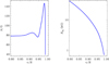 |
Fig. 1. Normalised buoyancy frequency (left panel) and equipartition field strength of Eq. (6) (right panel) in the near-surface region of about 20% of the star in radius. The plots correspond to the rotation period of 10 days. |
of the equality ΩA = Ω is also shown in Fig. 1.
Figure 2 shows profiles of three basic diffusivities in the radiation zone of the star. The magnetic diffusivity η = 1013T−3/2 cm2 s−1 (see e.g. Sect. 3.2 in Brandenburg & Subramanian 2005) computed for the profile of temperature T supplied by the stellar structure model corresponds to the characteristic time of the Ohmic decay (∼10 Gyr) exceeding the age of the star. The results of the following section refer to the steady background field of Eq. (1). Tayler instability is nevertheless sensitive to an interplay between thermal and magnetic diffusion (Spruit 1999).
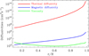 |
Fig. 2. Radial profiles of the microscopic viscosity and thermal and magnetic diffusivities in the radiation zone of the star. |
Instability in the upper part of the radiation zone can be relevant to surface observations. The diffusivity parameters of Eq. (4) estimated for the radius r = 0.9R read
 (7)
(7)
Computations for the most interesting case of super-equipartition background field (ΩA ≥ Ω) can be performed with this large spread in the diffusion parameters. However, the problem is that computations for the subequipartition case of ΩA < Ω are not feasible with the large contrast between thermal and magnetic diffusion of Eq. (7). Only with the thermal diffusivity reduced by about three orders of magnitude were computations for the weak-field case possible. Results in the following section therefore refer to the two cases of the diffusivities of Eq. (7) for ΩA ≥ Ω and to the reduced parameter of thermal diffusion ϵχ = 10−4 for a wider range of ΩA including subequipartition fields.
3. Results and discussion
Figure 3 shows drift rates of the most rapidly growing (dominant) instability mode in an inertial reference frame where the drift rates are equal to the observable rate of rotation of the instability pattern. The corresponding growth rates are shown in Fig. 4. For the subequipartition field strength of ΩA/Ω < 1, the normalised drift rates are only marginally smaller than one, signifying a co-rotation of the instability pattern with the star. The growth rates for the subequipartition background field scale as  (Spruit 1999). The scaling evidences a stabilising effect of rotation on Tayler instability.
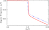 |
Fig. 3. Drift rate of the most rapidly growing instability mode measured in units of the angular velocity of the star as a function of the normalised amplitude of the background field of Eq. (1). The dashed line corresponds to the diffusion parameters of Eq. (7) and the full line corresponds to the reduced thermal diffusion of ϵχ = 10−4. |
The most pronounced changes in Figs. 3 and 4 are localised around the equipartition value of the field of ΩA = Ω. The drift rate decreases and the growth rate increases sharply with the field strength around this value. Instability of the strong fields with ΩA > Ω is fast, its growth rate scales as γ ∝ ΩA. The scaling shows that Tayler instability of strong fields is not sensitive to rotation. Unstable disturbances of strong fields avoid the stabilising effect of rotation by a counter-rotation drift. The drift rates of Fig. 3 approach the power law
 (8)
(8)
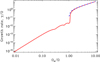 |
Fig. 4. Fractional growth rate of the instability as a function of the normalised amplitude of the background field of Eq. (1). The dashed line corresponds to the diffusion parameters of Eq. (7) and the full line corresponds to the reduced thermal diffusion of ϵχ = 10−4. |
for increasingly strong super-equipartition fields. The small coefficient c in this equation depends on the model parameters: c ≃ 0.037 and c ≃ 0.022 for the dashed and full lines of Fig. 3, respectively.
The almost resting eigenmodes for super-equipartition fields is a robust result; it was found for all considered parameter values and different profiles of the background field (Rüdiger & Kitchatinov 2010). The counter-rotational drift was also found by Bonanno & Urpin (2013b). Oscillation frequencies in the co-rotating frame of Figs. 1 to 3 by Bonanno & Urpin (2013b) are negative and vary in direct proportion to the angular velocity for the super-equipartition fields of ΩA > Ω.
Two types of eigenmodes that differ in their equatorial symmetry can be distinguished. The modes with equator-symmetric flow and entropy have an equator-antisymmetric magnetic pattern. This combination is caused by the anti-symmetry of the background field in Eq. (1). The other symmetry type combines anti-symmetric flow and entropy with a symmetric magnetic field. In our computations, modes of either symmetry type have almost the same growth rate and the same drift. Figures 3 and 4 can be attributed to either symmetry type.
The potentially observable patterns of the two types of equatorial symmetry are shown in Figs. 5 and 6. The reason for coincidence of the corresponding drift and growth rates can be seen from these figures. The eigenmodes of Figs. 5 and 6 are concentrated to poles and they are small near the equator. Their cross-equatorial link is therefore weak leading to practically indistinguishable eigenvalues of the two symmetry types. The patterns of these two symmetry types are very similar if viewed from a small inclination angle to the rotation axes.
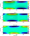 |
Fig. 5. Structure of the most rapidly growing mode combining the equator-symmetric magnetic field with equator-antisymmetric velocity and entropy patterns, all for ΩA/Ω = 1.5. Top panel: magnetic field pattern: full (dashed) lines show the clockwise (anti-clockwise) circulation of the toroidal field vector and the colour scale indicates the radial component of the field. Middle panel: similar pattern for the velocity field. Thermal (entropy) disturbances are shown in the bottom panel. Colour scales are graduated in arbitrary units. |
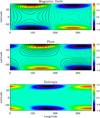 |
Fig. 6. Same as in Fig. 5 but for the mode combining the equator-antisymmetric magnetic field with equator-symmetric flow and entropy. |
It may be noted that any superposition of the eigenmodes of Figs. 5 and 6 has the same rates of growth and drift. The same is true for the patterns in Figs. 5 and 6 when shifted in longitude by arbitrary phase. Any superposition of eigenmodes of different symmetry or phase therefore gives a mode with the same eigenvalue. The superpositions make up patterns of different complexity that may explain the diversity of observed magnetic patterns. In this context, an interpretation by Mathys et al. (2016) of the unusual magnetic structure of SSRAp star HD 18078 in terms of a superposition of more simple magnetic configurations can be quoted.
Comparison of the magnetic periods with the rotational periods determined spectroscopically could be an observational test of our hypothesis. However, the difficulty is that SSRAp stars usually possess negligible spectroscopic signatures of rotation. The lines in their spectra are narrow but split magnetically (Mathys 2019). Due to uncertainty in sin i, this can be interpreted as either a result of slow proper rotation of the star or its closeness to pole-on orientation. Babcock et al. (1960) suggested that the subgroup of the so-called ‘sharp-lined Ap stars’ is formed by stars observed under small inclination angles. Such an interpretation does not contradict the picture suggested by our model. Indeed, the polar magnetic patterns of Figs. 5 and 6 are more easily observed with a pole-on orientation. Rotational modulation of their magnetic zones remains detectable with small but finite inclination angles.
A SSRAp star V1291 Aql (HD 188041) can serve as an illustrative example. A true rotational profile can be extracted from high-resolution spectra of this star with sophisticated modeling techniques. Romanovskaya et al. (2019) determined the fundamental parameters of V1291 Aql using a spectrum synthesised with a magnetic computational code. Their value for the projected rotational velocity of the star’s matter is V sin i = 2 km s−1 and radius R = 2.4 R⊙. Even with a large inclination angle of i = 90°, this leads to a proper rotation period of about 60 days, which is about four times shorter than the 224 days inferred by Mathys (2019) from the star’s magnetic variability. A small inclination of i ≃ 10° leads to a ‘normal’ value of Prot ≃ 10 days. This example is in favor of our explanation of the SSRAp phenomenon.
4. Conclusions
The angular frequency of Tayler instability eigenmodes can be very small (Fig. 3). If the instability does indeed shape the surface pattern of the magnetic field of the Ap stars (Arlt & Rüdiger 2011b; Spruit 2002), then rotation periods inferred from magnetic (or photometric) variability can exceed ten or even one hundred times the period of the stars’ proper rotation. The combined effect of the near pole-on orientation and the azimuthal drift of the magnetic pattern due to Tayler instability could explain the observational phenomenon of SSRAp stars (Mathys 2017, 2019).
Tayler instability has a low bound of several hundred Gauss for unstable fields. The low bound could also be the cause of the magnetic dichotomy found by Aurière et al. (2007).
These explanations, if confirmed, point to Tayler instability as the mechanism forming the magnetic fields of Ap stars.
The slow rotation of the instability pattern is reproduced for a background field strength exceeding the equipartition value of Eq. (6). The equipartition strength decreases with the proper rotation period of a star. The equipartition field of Fig. 1 is estimated for Prot = 10 days, and should be reduced in inverse proportion to Prot for longer rotation periods. The super-slow rotation of the instability pattern is therefore easier to reproduce (with a weaker background field) in slower rotators.
There are several directions for improvement of our theoretical model (waiving local approximation in radius, including nonlinearities, etc.). Nevertheless, we believe that the results of our model can be offered for a discussion prior to time-consuming advancements.
Acknowledgments
This work was supported by the Russian Foundation for Basic Research (project 17-52-80064_BRICS) and by budgetary funding of the Basic Research programme II.16.
References
- Arlt, R., & Rüdiger, G. 2011a, MNRAS, 412, 107 [NASA ADS] [CrossRef] [Google Scholar]
- Arlt, R., & Rüdiger, G. 2011b, Astron. Nachr., 332, 70 [NASA ADS] [CrossRef] [Google Scholar]
- Aurière, M., Wade, G. A., Silvester, J., et al. 2007, A&A, 475, 1053 [NASA ADS] [CrossRef] [EDP Sciences] [Google Scholar]
- Babcock, H. W. 1960, in Stellar Magnetic Fields, in Stellar Atmospheres, ed. J. L. Greenstein (Chicago Univ. Press), 282 [Google Scholar]
- Bonanno, A., & Urpin, V. 2013a, ApJ, 766, 52 [NASA ADS] [CrossRef] [Google Scholar]
- Bonanno, A., & Urpin, V. 2013b, MNRAS, 431, 3663 [NASA ADS] [CrossRef] [Google Scholar]
- Braithwaite, J. 2006, A&A, 453, 687 [NASA ADS] [CrossRef] [EDP Sciences] [Google Scholar]
- Brandenburg, A., & Subramanian, K. 2005, Phys. Rep., 417, 1 [NASA ADS] [CrossRef] [Google Scholar]
- Chandrasekhar, S. 1961, Hydrodynamic and hydromagnetic stability (Oxford: Clarendon Press) [Google Scholar]
- Goossens, M., Biront, D., & Tayler, R. J. 1981, Ap&SS, 75, 521 [NASA ADS] [CrossRef] [Google Scholar]
- Guerrero, G., Del Sordo, F., Bonanno, A., & Smolarkiewicz, P. K. 2019, MNRAS, 490, 4281 [NASA ADS] [CrossRef] [Google Scholar]
- Kitchatinov, L., & Rüdiger, G. 2008, A&A, 478, 1 [NASA ADS] [CrossRef] [EDP Sciences] [Google Scholar]
- Mathys, G. 2017, A&A, 601, A14 [NASA ADS] [CrossRef] [EDP Sciences] [Google Scholar]
- Mathys, G. 2019, ArXiv e-prints [arXiv:1912.06107] [Google Scholar]
- Mathys, G., Romanyuk, I. I., Kudryavtsev, D. O., et al. 2016, A&A, 586, A85 [NASA ADS] [CrossRef] [EDP Sciences] [Google Scholar]
- Mathys, G., Romanyuk, I. I., Hubrig, S., et al. 2019, A&A, 629, A39 [NASA ADS] [CrossRef] [EDP Sciences] [Google Scholar]
- Paxton, B., Bildsten, L., Dotter, A., et al. 2011, ApJS, 192, 3 [Google Scholar]
- Romanovskaya, A., Ryabchikova, T., Shulyak, D., et al. 2019, MNRAS, 488, 2343 [CrossRef] [Google Scholar]
- Rüdiger, G., & Kitchatinov, L. L. 2010, Geophys. Astrophys. Fluid Dyn., 104, 273 [CrossRef] [Google Scholar]
- Rüdiger, G., Kitchatinov, L. L., & Elstner, D. 2012, MNRAS, 425, 2267 [NASA ADS] [CrossRef] [Google Scholar]
- Spruit, H. C. 1999, A&A, 349, 189 [NASA ADS] [Google Scholar]
- Spruit, H. C. 2002, A&A, 381, 923 [NASA ADS] [CrossRef] [EDP Sciences] [Google Scholar]
- Tayler, R. J. 1973, MNRAS, 161, 365 [NASA ADS] [CrossRef] [Google Scholar]
- Watson, M. 1981, Geophys. Astrophys. Fluid Dyn., 16, 285 [Google Scholar]
- Zahn, J. P., Brun, A. S., & Mathis, S. 2007, A&A, 474, 145 [NASA ADS] [CrossRef] [EDP Sciences] [Google Scholar]
All Figures
|
Fig. 1. Normalised buoyancy frequency (left panel) and equipartition field strength of Eq. (6) (right panel) in the near-surface region of about 20% of the star in radius. The plots correspond to the rotation period of 10 days. |
| In the text | |
|
Fig. 2. Radial profiles of the microscopic viscosity and thermal and magnetic diffusivities in the radiation zone of the star. |
| In the text | |
|
Fig. 3. Drift rate of the most rapidly growing instability mode measured in units of the angular velocity of the star as a function of the normalised amplitude of the background field of Eq. (1). The dashed line corresponds to the diffusion parameters of Eq. (7) and the full line corresponds to the reduced thermal diffusion of ϵχ = 10−4. |
| In the text | |
|
Fig. 4. Fractional growth rate of the instability as a function of the normalised amplitude of the background field of Eq. (1). The dashed line corresponds to the diffusion parameters of Eq. (7) and the full line corresponds to the reduced thermal diffusion of ϵχ = 10−4. |
| In the text | |
|
Fig. 5. Structure of the most rapidly growing mode combining the equator-symmetric magnetic field with equator-antisymmetric velocity and entropy patterns, all for ΩA/Ω = 1.5. Top panel: magnetic field pattern: full (dashed) lines show the clockwise (anti-clockwise) circulation of the toroidal field vector and the colour scale indicates the radial component of the field. Middle panel: similar pattern for the velocity field. Thermal (entropy) disturbances are shown in the bottom panel. Colour scales are graduated in arbitrary units. |
| In the text | |
|
Fig. 6. Same as in Fig. 5 but for the mode combining the equator-antisymmetric magnetic field with equator-symmetric flow and entropy. |
| In the text | |
Current usage metrics show cumulative count of Article Views (full-text article views including HTML views, PDF and ePub downloads, according to the available data) and Abstracts Views on Vision4Press platform.
Data correspond to usage on the plateform after 2015. The current usage metrics is available 48-96 hours after online publication and is updated daily on week days.
Initial download of the metrics may take a while.