| Issue |
A&A
Volume 637, May 2020
|
|
|---|---|---|
| Article Number | A42 | |
| Number of page(s) | 7 | |
| Section | The Sun and the Heliosphere | |
| DOI | https://doi.org/10.1051/0004-6361/201936836 | |
| Published online | 12 May 2020 | |
Transverse oscillations of a double-structured solar filament⋆
1
University of South Bohemia, Faculty of Science, Institute of Physics, Branišovská 1760, 370 05 České Budějovice, Czech Republic
e-mail: This email address is being protected from spambots. You need JavaScript enabled to view it.
2
Astronomical Institute of the Czech Academy of Sciences, Fričova 258, 251 65 Ondřejov, Czech Republic
3
Central (Pulkovo) Astronomical Observatory, Russian Academy of Sciences, Pulkovskoe Shausse 65, 196140 St. Petersburg, Russia
4
Crimean Astrophysical Observatory of the Russian Academy of Sciences Nauchny Russia, Russia
Received:
3
October
2019
Accepted:
27
March
2020
Abstract
Aims. We study the transverse oscillations of a double-structured solar filament.
Methods. We modelled the filament numerically via a 2D magnetohydrodynamic (MHD) model, in which we solved a full set of time-dependent MHD equations by means of the FLASH code, using the adaptive mesh refinement method. We used the wavelet analysis method as a diagnostic tool for analysing periods in simulated oscillations.
Results. We present a model of a solar filament combined with semi-empirical C7 model of the quiet solar atmosphere. This model is an alternative model of a filament based on the magnetostatic solution of MHD equations. We find that this double-structured filament oscillates with two different eigen frequencies. The ratio is approximately 1.75 (∼7.4 min/∼4.2 min), which is characteristic for this type of filament model. To show the details of these oscillations we present a time evolution of the plasma density, temperature, plasma beta parameter, and the ratio of gravity to magnetic pressure taken along the vertical axis of the filament at x = 0. The periods found by numerical simulations are then discussed in comparison with those observed.
Key words: Sun: filaments, prominences / Sun: oscillations / magnetohydrodynamics (MHD) / methods: numerical
The movie associated to Fig. 3 is available at https://www.aanda.org
© ESO 2020
1. Introduction
Solar filaments seen in Hα or extreme ultraviolet (EUV) observations (against the solar disc) appear as dark ribbons (Tandberg-Hanssen 1995; Foukal 2004; Priest 2014; Vial & Oddbjørn 2015; Arregui et al. 2018). Filaments, which are very complex structures of plasma threaded by magnetic fields, are composed of dense (1017 − 1018 m−3) and cold (104 K) plasma, floated in the tenuous (1014 − 1015 m−3) and hot (106 K) solar coronal plasma. Several models of filaments with various magnetic field configurations have been suggested in the literature. Besides the classical models (Kippenhahn & Schlüter 1957; Kuperus & Raadu 1974), in which the magnetic tension provides an upward force to balance the gravity or this balance is due to the Lorentz force produced by the mirror electric current under the photosphere, there are new models that combine these forces. These models have one dense filament or two dense filaments, that is, the so-called double-decker filament. This double-decker filament was proposed in two forms. The first form has a single flux rope on top of a sheared arcade and the second form has two flux ropes; see Fig. 12 in Liu et al. (2012) and the numerical simulations in Kliem et al. (2014). The filament configuration with the twisted flux rope above the sheared magnetic arcade has also been proposed by Awasthi et al. (2019), who analysed mass motions inside the filament. We note that in these models the magnetic field in the arcade and the rope at their interaction region, as well as between two ropes, are oppositely orientated.
The filaments are often observed as oscillating structures. Hence, they offer various type of oscillations with a range of periods from tens of seconds to tens of minutes (Oliver & Ballester 2002) or even many hours (Foullon et al. 2004, 2009; Pouget et al. 2006; Efremov et al. 2016; Arregui et al. 2018). We recognise two types of their oscillations: longitudinal or transverse. Longitudinal oscillations are excited, for example by jets or shocks at footpoints of the filament propagating along the filament. Transverse oscillations can be generated, for example by a shock wave propagating from the lower parts of the solar atmosphere and colliding with the filament (Awasthi et al. 2019) and references therein.
Filament oscillations have been numerically studied in many papers. Recently, using a full 3D MHD model with a dense filament embedded in a magnetic rope, Zhou et al. (2018) found that the longitudinal oscillation has a period of about 49 min in accordance with the pendulum filament model. The horizontal transverse oscillation has a period of about 10 min and the vertical transverse oscillation has a period of about 14 min, and both of these agree with a 2D slab model. The transverse and longitudinal filament oscillations have also been studied in a 3D curtain-shaped model (Adrover-González & Terradas 2020).
Besides all these filament models, there is the model by Solov’ev (2012), which consists of an upper rope with a dense and cool plasma and lower rope, which is rarefied and hot. The magnetic field between these two ropes does not change the sign.
In the present paper we combine the Solov’ev model with the Avrett & Loeser C7 model, which is a hydrostatic model of the solar atmosphere (Avrett & Loeser 2008). We call this model the double-structured model of a filament in an initial state of equilibrium. We impose, on this model, a lateral perturbation in the form of a pulse having the form of a Gaussian of a given width and amplitude. The main aim of the present paper is to numerically study the transverse oscillations arising in this perturbed double-structured filament configuration and compare these with observations.
The structure of the paper is as follows. In Sect. 2 we present the numerical model with its initial equilibrium and perturbation. Then the results of numerical simulations and wavelet analysis are shown. Finally, in Sect. 3, we discuss the results obtained.
2. Numerical model
We numerically solved the 2D, time-dependent, ideal magnetohydrodynamic (MHD) equations in their form, described in our previous papers (e.g. Jelínek & Murawski 2013; Jelínek et al. 2015; Murawski et al. 2018). In brief, our numerical model solves the equation of conservation of mass, momentum, energy, and the induction equation.
We solved this set of MHD equations via the FLASH code1 (Lee & Deane 2009), which is a multi-physics, open science simulation code that is well tested, fully modular, and parallel. This code implements second- and third-order unsplit Godunov solvers with various slope limiters and Riemann solvers as well as adaptive mesh refinement (AMR; e.g. Chung 2002). The main advantage of using AMR technique is to refine a numerical grid at steep spatial profiles while keeping a grid coarse in areas where fine spatial resolution is not essential. In our case, the AMR strategy is based on controlling the numerical errors in a gradient of mass density that leads to a reduction of the numerical diffusion within the entire simulation region.
For our numerical simulations, we set a 2D simulation box as ( − 10, 10) Mm × (0,20) Mm (see Fig. 1). The spatial resolution of the numerical grid is determined by the AMR method. We used the AMR grid with the minimum (maximum) level of the refinement blocks set to 2 (6). The whole simulation region is covered by 2852 blocks. Since every block consists of 8 × 8 numerical cells, this number of blocks corresponds to 182528 numerical cells, and the smallest spatial resolution is Δx = Δy = 0.0391 Mm. At all boundaries, we fixed all of the plasma quantities to their equilibrium values, which lead only to negligibly small numerical reflections of incident wave signals.
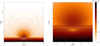 |
Fig. 1. Sketch of the initial mass density distribution (t = 0) with representative magnetic field lines shown as grey solid lines (left). The black rectangle shows the zoomed area visible in detail in the right part of the figure. The white solid line separates the upper and lower magnetic ropes and the black circles indicate the detection points. |
Generally, the terms expressing the radiative losses Rloss, thermal conduction Tcond, and heating H should be added to the set of MHD equations. In the initial state it is assumed that the radiative losses and thermal conduction are fully compensated by the heating H (i.e. Rloss + Tcond + H = 0), otherwise the unperturbed atmosphere is not in equilibrium, for example owing to the steep temperature gradient in the transition region (TR). Problems appear when the atmosphere is perturbed. Namely, there is no simple expression for the heating term H, which in the unperturbed atmosphere fully compensates Rloss and Tcond, and in the perturbed atmosphere correctly describes the heating. Therefore, for the purpose of our study, we assumed that Rloss + Tcond + H = 0 is valid during the whole studied processes.
For the wavelet analysis of wave signal we used the Morlet wavelet, which consists of a plane wave modulated by a Gaussian,
 (1)
(1)
where the parameter σ allows for a trade between time and frequency resolutions. In this equation, we assumed the value of parameter σ = 6, as recommended by Farge (1992). The wave periods were estimated from the global wavelet spectrum as the most dominant period in this spectrum. More details about the wavelet method and its implementation can be found, for example in Farge (1992) and Torrence & Compo (1998).
2.1. Initial equilibrium
For a still (v = 0) equilibrium, the Lorentz and gravity forces have to be balanced by the pressure gradient in the entire physical domain
 (2)
(2)
where
 (3)
(3)
The solenoidal condition, ∇ ⋅ B = 0, is identically satisfied with the implementation of the magnetic flux function, A, such as
 (4)
(4)
In the case of a 2D magnetic field we used A = [0, 0, A], where
 (5)
(5)
where k2 = (5.0 Mm)−1 is a free parameter, which defines the scale of the system, and B0 = 10−3 T is the magnetic field at h0 = 1.8 Mm, which is the height of the centre of the double-filament structure above the solar surface. From Eq. (4) it follows then that the magnetic field components (Bx, By, 0) are given by
![Mathematical equation: $$ \begin{aligned}&B_x = B_0\frac{[1+k^2x^2-k^2(y-h_0)^2]}{[1+k^2x^2+k^2(y-h_0)^2]^2}, \end{aligned} $$](/articles/aa/full_html/2020/05/aa36836-19/aa36836-19-eq6.gif) (6)
(6)
![Mathematical equation: $$ \begin{aligned}&B_y = -B_0\frac{2k^2x(y-h_0)}{[1+k^2x^2+k^2(y-h_0)^2]^2}\cdot \end{aligned} $$](/articles/aa/full_html/2020/05/aa36836-19/aa36836-19-eq7.gif) (7)
(7)
The equilibrium gas pressure, p, and mass density, 𝜚, are generally expressed as (Solov’ev 2010)
![Mathematical equation: $$ \begin{aligned}&p(x,y) = p_{\rm h}(y) - \frac{1}{\mu _0}\left[\int \limits _{x}^{\infty }\frac{\partial ^2 A}{\partial y^2}\frac{\partial A}{\partial x}\mathrm{d}x + \frac{1}{2}\left(\frac{\partial A}{\partial x}\right)^2\right], \end{aligned} $$](/articles/aa/full_html/2020/05/aa36836-19/aa36836-19-eq8.gif) (8)
(8)
![Mathematical equation: $$ \begin{aligned}&\varrho (x,y) = \varrho _{\rm h}(y) + \frac{1}{\mu _0 g_{\odot }}\Bigg \{\frac{\partial }{\partial {y}}\Bigg [\int \limits _{x}^{\infty } \frac{\partial ^2 A}{\partial y^2}\frac{\partial A}{\partial x}\mathrm{d}x\nonumber \\&\qquad \qquad +\frac{1}{2}\Bigg (\frac{\partial A}{\partial x}\Bigg )^2\Bigg ] - \frac{\partial A}{\partial y} \nabla ^2 A\Bigg \}, \end{aligned} $$](/articles/aa/full_html/2020/05/aa36836-19/aa36836-19-eq9.gif) (9)
(9)
where
![Mathematical equation: $$ \begin{aligned}&p_{\rm h}(y) = p_0 \exp \left[-\int \limits _{y_0}^{y} \frac{1}{\Lambda (\tilde{y})}\mathrm{d}\tilde{y}\right], \end{aligned} $$](/articles/aa/full_html/2020/05/aa36836-19/aa36836-19-eq10.gif) (10)
(10)
 (11)
(11)
are the hydrostatic gas pressure and mass density, respectively, and p0 denotes the gas pressure at the reference level y0.
The pressure scale-height, which in the case of isothermal atmosphere represents the vertical distance over which the gas pressure falls off by the factor of e, is expressed by
 (12)
(12)
where kB = 1.38 × 10⁻²³ J K−1 is the Boltzmann constant and  is the mean particle mass (mp = 1.672 × 10⁻²⁷ kg, is the proton mass). For the solar atmosphere, the temperature profile, T(y), was derived by Avrett & Loeser (2008). At the top of the photosphere, which corresponds to height y = 0.5 Mm, the temperature is T(y) = 5700 K. At higher altitudes, the temperature falls off to its minimal value T(y) = 4350 K at y ≈ 0.95 Mm. Higher up the temperature rises very slowly to the height about y = 2.7 Mm, where the TR is located. The temperature increases abruptly to the value, T(y) = 1.5 MK, at the altitude y = 10 Mm, which is typical for the solar corona.
Substituting Eq. (5) into Eqs. (8) and (9) we get for the gas pressure
 (13)
(13)
and for the mass density
![Mathematical equation: $$ \begin{aligned} \varrho (x,y) = \varrho _{\rm h}(y) + \frac{B_0^2}{2 \mu g_{\odot }}\cdot \frac{8k^2(y-h_0)}{[1+k^2x^2+k^2(y-h_0)^2]^4}, \end{aligned} $$](/articles/aa/full_html/2020/05/aa36836-19/aa36836-19-eq15.gif) (14)
(14)
where
![Mathematical equation: $$ \begin{aligned} B_z^2(A) = B_{\rm ex}^2 - \alpha ^2 B_0^2\left\{ \frac{k(y-h_0)}{[1+k^2x^2+k^2(y-h_0)^2]}\right\} ^2. \end{aligned} $$](/articles/aa/full_html/2020/05/aa36836-19/aa36836-19-eq16.gif) (15)
(15)
In this equation, α is an arbitrary positive constant and Bex is an external magnetic field at infinity. The condition for the external magnetic field is Bex > (αB0)/2 and Bz(0) = Bex = 10−3 T. On the left side of Fig. 1 we show the distribution of the initial mass density at t = 0 s with representative magnetic field lines. On the right side of this figure we can see the white solid line which separates the upper and lower magnetic ropes and the black circles indicate the detection points. The vertical profiles of the Bx component of magnetic field, mass density, and temperature along the axis of symmetry (x = 0 Mm) in the initial state are shown in Fig. 2.
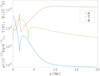 |
Fig. 2. Vertical profiles of the Bx component of magnetic field (green line), mass density (blue line), and temperature (red line) along the axis of symmetry (x = 0 Mm) in the initial state. |
2.2. Perturbation
At the start of the numerical simulations, at t = 0 s, the equilibrium is perturbed by the Gaussian pulse of the following form:
![Mathematical equation: $$ \begin{aligned} v_x(x,y,t=0) = -A_0\frac{x}{\lambda }\exp \left[-\frac{x^2 + (y-y_{\mathrm{P}})^2}{\lambda ^2}\right], \end{aligned} $$](/articles/aa/full_html/2020/05/aa36836-19/aa36836-19-eq17.gif) (16)
(16)
where A0 = 0.05 cA(x = 0, y = y0) is the initial amplitude of the pulse, yP = 1.8 Mm is the vertical position of the pulse, and λ = 0.5 Mm is the pulse width.
3. Numerical results
Prior to performing the numerical simulations, we verified through a simulation test that the system remains in numerical equilibrium for the adopted grid resolution, while not being perturbed by any velocity pulse. This can be realised by setting A0 = 0 in Eq. (16). This test shows that the numerically induced flow is very small within the whole simulation region over duration of the numerical experiment; the largest value of this flow is found right above the TR and is about 3 km s−1, which is much less than the characteristic speeds that we observe there. After performing this basic numerical test we started to simulate the system dynamics by launching the initial pulse in a horizontal component of velocity, according to Eq. (16).
The time series of the snapshots from the simulation run is presented in Fig. 3. In all figures, the mass density distribution in logarithmic scale is shown, along with the magnetic field lines drawn as grey solid lines. We chose only some snapshots for several periods of oscillations at times t = 130, 230, 350, 500, 630, and 1140 s, where we can observe the dynamics of the whole complex structure. Shortly after the initial horizontal velocity pulse, the plasma from lower parts of the solar atmosphere starts to move up (t = 130 s) and the magnetic field lines start to be deformed. The snapshot for the time t = 230 s shows the ejected material falling down back to denser parts of the solar atmosphere and appropriate changes in the shape of the magnetic field lines. This process is repeated several times (snapshots for times t = 350−1140 s) and then is gradually attenuated in time. From the dynamics of the system we find two main oscillation periods. The movie from the simulation is available online.
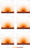 |
Fig. 3. Time series of snapshots from the numerical simulation. An animation of this figure, showing the whole temporal evolution of the double-filament, is available online. |
In Fig. 4 we show the wave signal (changes in mass density) and the corresponding wavelet power spectrum (left); the global wavelet spectrum shows the period (right) for three different detection points. We chose these points in the center of rare filament, dense filament, and in the position of the minimal magnetic field in the upper rope, respectively (see also the profiles in Fig. 2). From the wave signal we make the wavelet analysis and estimate the period of oscillations. We can clearly see that for all detection points there are two main periods about ≈4.2 min and ≈7.4 min.
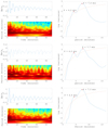 |
Fig. 4. Wave signal and corresponding wavelet power spectrum (left) and the global wavelet spectrum showing the period (right). The red dashed line designates the cone of influence of the wavelet spectrum. The results are shown for three different detection points placed in the axis of the symmetry: see the black circles in Fig. 1. |
To understand these oscillations better in Fig. 5 we present a time evolution of the plasma density, temperature, plasma beta parameter, and the ratio of gravity to magnetic pressure taken along the vertical axis of the filament at x = 0 Mm. As shown in this figure, the oscillations are not strictly sinusoidal, which agrees with two eigen periods (∼7.4 min and ∼4.2 min) detected by the wavelet analysis. This is also in agreement with the time profiles of density variations shown in Fig. 4. However, it differs from sinusoidal variations of the parameters shown in Zhou et al. (2018), Adrover-González & Terradas (2020). This difference appears to be caused by the different structure of the filament. While in Zhou et al. (2018), Adrover-González & Terradas (2020) there is one single dense filament, in this work we are studying a double-structured filament.
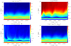 |
Fig. 5. Time evolution of the plasma density, temperature, plasma beta parameter, and the ratio of gravity to magnetic pressure along the axis of filament (x = 0 Mm) in log10 scale. |
Furthermore, as seen in this figure, for example at time t ∼ 470 s and y = 2.5 Mm, the density increase is synchronised with the increase of the temperature and plasma beta parameter. The plasma beta parameter in the region y = 1−5 Mm, which is the most important for oscillations, is lower than one (log10 lower than 0). Thus, for the detected oscillations the magnetic force is dominant. This conclusion is also confirmed by the time evolution of the ratio of gravity to magnetic pressure. We can see that in the lower layers of the solar atmosphere, gravity is dominant, whereas the magnetic force prevails in layers for which we study the oscillations. In these layers of oscillations, the mentioned ratio is lower than one (in a logarithmic scale lower than zero), which indicates that the magnetic pressure is much more important than gravity.
4. Discussion and conclusions
In the paper we present an alternative model of the solar filament. This model combines the Solov’ev filament model with the Avrett and Loeser C7 model of the solar atmosphere. It follows from the magnetostatic solution of MHD equations. This model is double-structured, consisting of an upper rope, which is embedded with dense and cool plasma, and a bottom rope, which is rarefied and hot. In the numerical simulation, using the FLASH code, we studied its transverse oscillations.
This model differs in some aspects from the other models mentioned in the Introduction. The most similar model is that in which a single flux rope is on top of a sheared arcade, such as in the model shown in Awasthi et al. (2019). However, it should be emphasised that in this model the magnetic field changes its sign at the bottom boundary of the magnetic flux ropes. Such a configuration does not guarantee the initial equilibrium in the system. Inevitably, reconnections of magnetic field lines should occur, which destroy the field structure. An advantage of the present model is that it is formulated as the physical model in equilibrium in the initial state. In our model, there are no magnetic fields of opposite polarity. The magnetic field at all points in space is uniquely determined by the analytic function, which does not provide the contact of fields of opposite polarity, and the external overlying field is not assumed. There are no singular or null-points inside the system, so there is no reason to assume the presence of any reconnections of magnetic field lines. It should be mentioned that our model system does not fall apart with an external disturbance, but begins to oscillate around its equilibrium position. In this double-structured filament model we found oscillations with two distinct periods 7.4 min and 4.2 min, which gives their ratio 1.75. These periods are nearly the same in all heights inside the filament. Therefore, these two periods are not the period of the top and bottom ropes separately, but it looks as though the periods are those of the whole coupled system.
Looking into details of these oscillations we found that the oscillations are not strictly sinusoidal. This agrees with the detection of two different periods (∼7.4 min and ∼4.2 min). In this regard, oscillations in the present model differ from sinusoidal variations of the parameters shown in Zhou et al. (2018), Adrover-González & Terradas (2020). This difference appears to be caused by the different structure of the filament. While in Zhou et al. (2018), Adrover-González & Terradas (2020) there is one single dense filament, we are studying a double-structured filament. Thus, these two frequencies with their ratio (∼1.75) could be one criterium for verification of the reality of a double-structured filament.
We found that the plasma beta parameter in the region, which is the most important for oscillations, is lower than one; we also confirmed that the ratio of gravity to magnetic pressure is also lower than one (in a logarithmic scale lower than zero). From this, we can conclude that for the detected oscillations the magnetic force is dominant.
We searched, in published papers based on observations, for periods of transverse filament oscillations that are similar to those found in our simulations. Yi et al. (1991) study observations of two quiescent filaments, which show oscillatory variations in Doppler shift and central intensity of the He I λ = 10830 Å line. The Doppler shift for the filament on the solar disc expresses the transverse filament oscillations. These authors analysed these oscillations and found the periods in the range 5−15 min, with dominant periods of 5, 9, and 16 min. The 5 and 9 min periods roughly agree with those in the present simulations.
Movie
Movie of Fig. 3 Access Supplementary Material
Acknowledgments
The authors thank the unknown referee for the constructive comments that improved the paper. P. J. expresses his thanks to Professor Krzystof Murawski from UMCS Lublin in Poland, for the valuable discussions and for the financial support when he worked on this paper during his stay in June 2019. A. S. thanks the Russian Scientific Foundation for the support of the work (project 15-12-20001). M. K. acknowledges support from Project RVO:67985815 and Grants 18-09072S, 19-09489S and 20-09922J of the Grant Agency of the Czech Republic. The FLASH code used in this work was developed by the DOE-supported ASC/Alliances Center for Astrophysical Thermonuclear Flashes at the University of Chicago. The wavelet analysis was performed using the software written by C. Torrence and G. Compo, http://paos.colorado.edu/research/wavelets.
References
- Adrover-González, A., & Terradas, J. 2020, A&A, 633, A113 [NASA ADS] [CrossRef] [EDP Sciences] [Google Scholar]
- Arregui, I., Oliver, R., & Ballester, J. L. 2018, Liv. Rev. Sol. Phys., 15, 3 [Google Scholar]
- Avrett, E. H., & Loeser, R. 2008, ApJS, 175, 229 [NASA ADS] [CrossRef] [Google Scholar]
- Awasthi, A. K., Liu, R., & Wang, Y. 2019, ApJ, 872, 109 [NASA ADS] [CrossRef] [Google Scholar]
- Chung, T. J. 2002, Computational Fluid Dynamics (Cambridge: Cambridge University Press) [CrossRef] [Google Scholar]
- Efremov, V. I., Parfinenko, L. D., & Solov’ev, A. A. 2016, Sol. Phys., 291, 3357 [NASA ADS] [CrossRef] [Google Scholar]
- Farge, M. 1992, Annu. Rev. Fluid Mech., 24, 395 [Google Scholar]
- Foukal, P. V. 2004, Solar Astrophysics, 2nd, Revised Edition (Wiley-VCH), 480 [CrossRef] [Google Scholar]
- Foullon, C., Verwichte, E., & Nakariakov, V. M. 2004, A&A, 427, L5 [NASA ADS] [CrossRef] [EDP Sciences] [Google Scholar]
- Foullon, C., Verwichte, E., & Nakariakov, V. M. 2009, ApJ, 700, 1658 [NASA ADS] [CrossRef] [Google Scholar]
- Jelínek, P., & Murawski, K. 2013, MNRAS, 434, 2347 [NASA ADS] [CrossRef] [Google Scholar]
- Jelínek, P., Srivastava, A. K., Murawski, K., Kayshap, P., & Dwivedi, B. N. 2015, A&A, 581, A131 [NASA ADS] [CrossRef] [EDP Sciences] [Google Scholar]
- Kippenhahn, R., & Schlüter, A. 1957, Z. Astrophys., 43, 36 [Google Scholar]
- Kliem, B., Török, T., Titov, V. S., et al. 2014, ApJ, 792, 107 [NASA ADS] [CrossRef] [Google Scholar]
- Kuperus, M., & Raadu, M. A. 1974, A&A, 31, 189 [NASA ADS] [Google Scholar]
- Lee, D., & Deane, A. E. 2009, J. Comput. Phys., 228, 952 [NASA ADS] [CrossRef] [Google Scholar]
- Liu, R., Kliem, B., Török, T., et al. 2012, ApJ, 756, 59 [NASA ADS] [CrossRef] [Google Scholar]
- Murawski, K., Kayshap, P., Srivastava, A. K., et al. 2018, MNRAS, 474, 77 [NASA ADS] [CrossRef] [Google Scholar]
- Oliver, R., & Ballester, J. L. 2002, Sol. Phys., 206, 45 [NASA ADS] [CrossRef] [Google Scholar]
- Pouget, G., Bocchialini, K., & Solomon, J. 2006, A&A, 450, 1189 [NASA ADS] [CrossRef] [EDP Sciences] [Google Scholar]
- Priest, E. 2014, Magnetohydrodynamics of the Sun (Cambridge: Cambridge University Press) [Google Scholar]
- Solov’ev, A. A. 2010, Astron. Rep., 54, 86 [NASA ADS] [CrossRef] [Google Scholar]
- Solov’ev, A. A. 2012, Geomagn. Aeron., 52, 1062 [NASA ADS] [CrossRef] [Google Scholar]
- Tandberg-Hanssen, E. 1995, The Nature of Solar Prominences (Dordrecht: Kluwer Academic Publishers), 199 [Google Scholar]
- Torrence, C., & Compo, G. P. 1998, Bull. Am. Meteorol. Soc., 79, 61 [Google Scholar]
- Vial, J. C., & Oddbjørn, E. 2015, in Solar Prominences (Switzerland: Springer International Publishing), Astrophys. Space Sci. Lib., 415 [CrossRef] [Google Scholar]
- Yi, Z., Engvold, O., & Keil, S. L. 1991, Sol. Phys., 132, 63 [NASA ADS] [CrossRef] [Google Scholar]
- Zhou, Y.-H., Xia, C., Keppens, R., Fang, C., & Chen, P. F. 2018, ApJ, 856, 179 [Google Scholar]
All Figures
|
Fig. 1. Sketch of the initial mass density distribution (t = 0) with representative magnetic field lines shown as grey solid lines (left). The black rectangle shows the zoomed area visible in detail in the right part of the figure. The white solid line separates the upper and lower magnetic ropes and the black circles indicate the detection points. |
| In the text | |
|
Fig. 2. Vertical profiles of the Bx component of magnetic field (green line), mass density (blue line), and temperature (red line) along the axis of symmetry (x = 0 Mm) in the initial state. |
| In the text | |
|
Fig. 3. Time series of snapshots from the numerical simulation. An animation of this figure, showing the whole temporal evolution of the double-filament, is available online. |
| In the text | |
|
Fig. 4. Wave signal and corresponding wavelet power spectrum (left) and the global wavelet spectrum showing the period (right). The red dashed line designates the cone of influence of the wavelet spectrum. The results are shown for three different detection points placed in the axis of the symmetry: see the black circles in Fig. 1. |
| In the text | |
|
Fig. 5. Time evolution of the plasma density, temperature, plasma beta parameter, and the ratio of gravity to magnetic pressure along the axis of filament (x = 0 Mm) in log10 scale. |
| In the text | |
Current usage metrics show cumulative count of Article Views (full-text article views including HTML views, PDF and ePub downloads, according to the available data) and Abstracts Views on Vision4Press platform.
Data correspond to usage on the plateform after 2015. The current usage metrics is available 48-96 hours after online publication and is updated daily on week days.
Initial download of the metrics may take a while.