| Issue |
A&A
Volume 636, April 2020
|
|
|---|---|---|
| Article Number | A117 | |
| Number of page(s) | 11 | |
| Section | Planets and planetary systems | |
| DOI | https://doi.org/10.1051/0004-6361/201937409 | |
| Published online | 29 April 2020 | |
Non-detection of TiO and VO in the atmosphere of WASP-121b using high-resolution spectroscopy
1
Astrophysics Research Centre, School of Mathematics and Physics, Queen’s University Belfast,
Belfast
BT7 1NN, UK
e-mail: This email address is being protected from spambots. You need JavaScript enabled to view it.
2
School of Physics, Trinity College Dublin,
Dublin 2, Ireland
3
Physikalisches Institut, Universität Bern,
Gesellschaftsstrasse 6,
3012
Bern, Switzerland
4
School of Chemistry, University of New South Wales,
2052
Sydney, Australia
5
Department of Physics and Astronomy, University College London,
Gower Street,
WC1E 6BT
London, UK
6
Department of Physics, Massachusetts Institute of Technology,
Cambridge,
MA
02139, USA
7
Department of Earth and Planetary Sciences, Johns Hopkins University,
Baltimore,
MD, USA
8
Physics and Astronomy, Stocker Road, University of Exeter,
Exeter,
EX4 3RF, UK
Received:
23
December
2019
Accepted:
4
February
2020
Abstract
Thermal inversions have long been predicted to exist in the atmospheres of ultra-hot Jupiters. However, the detection of two species thought to be responsible – titanium oxide and vanadium oxide – remains elusive. We present a search for TiO and VO in the atmosphere of the ultra-hot Jupiter WASP-121b (Teq ≳ 2400 K), an exoplanet with evidence of VO in its atmosphere at low resolution which also exhibits water emission features in its dayside spectrum characteristic of a temperature inversion. We observed its transmission spectrum with the UV-Visual Echelle Spectrograph at the Very Large Telescope and used the cross-correlation method – a powerful tool for the unambiguous identification of the presence of atomic and molecular species – in an effort to detect whether TiO or VO were responsible for the observed temperature inversion. No evidence for the presence of TiO or VO was found at the terminator of WASP-121b. By injecting signals into our data at varying abundance levels, we set rough detection limits of [VO] ≲−7.9 and [TiO] ≲−9.3. However, these detection limits are largely degenerate with scattering properties and the position of the cloud deck. Our results may suggest that neither TiO or VO are the main drivers of the thermal inversion in WASP-121b; however, until a more accurate line list is developed for VO, we cannot conclusively rule out its presence. Future works will consist of a search for other strong optically-absorbing species that may be responsible for the excess absorption in the red-optical.
Key words: planets and satellites: atmospheres / planets and satellites: individual: WASP-121b / methods: observational / techniques: spectroscopic
© ESO 2020
1 Introduction
An open question in the field of exoplanet atmospheres is that of the existence and origin of thermal inversions in hot Jupiters. It was postulated by Hubeny et al. (2003) and Fortney et al. (2008) that the hottest of hot Jupiters (Teq > 2000 K) would host titanium oxide and vanadium oxide in their gaseous form, which would strongly absorb ultra-violet and visible light and would heat the upper atmosphere, leading to a rise in temperature with altitude: hence, a thermal inversion. However, evidence for the existence of thermal inversions has proven unexpectedly difficult to discover. Direct detections of TiO or VO have been equally elusive.
The first evidence of an inversion layer was reported by Knutson et al. (2008) in the atmosphere of HD 209458b, using secondary eclipse observations from the Spitzer Space Telescope. However, the later work by Hansen et al. (2014) shows that several previous single-transit measurements made using Spitzer had much higher uncertainties than previously thought and work by Zellem et al. (2014), Diamond-Lowe et al. (2014), Schwarz et al. (2015), Evans et al. (2015), and Line et al. (2016) shows results consistent with no temperature inversion layer. Further studies find a surprising number of flat, blackbody-like emission spectra for a number of ultra-hot Jupiters (Swain et al. 2013; Cartier et al. 2017; Kreidberg et al. 2018; Arcangeli et al. 2018; Mansfield et al. 2018) showing none of the emission or absorption features that would indicate the presence of the expected temperature inversion. Sedaghati et al. (2017) report a detection of TiO in the ground-based transmission spectrum of WASP-19b using FORS2 (FOcal Reducer/low dispersion Spectrograph 2) on the Very Large Telescope, contradicting an earlier result from the Space Telescope Imaging Spectrograph on the Hubble Space Telescope (HST) that found no evidence of TiO (Huitson et al. 2013). However, a subsequent attempt to reproduce the detection using IMACS (Inamori Magellan Areal Camera and Spectrograph) on Magellan has proven unsuccessful (Espinoza et al. 2019). Haynes et al. (2015) observe the dayside of WASP-33b (Teq ~ 2700 K) at low resolution with Wide Field Camera 3 on HST and find a thermal emission feature at ~1 micron, consistent with the presence of TiO. This claim has been strengthened by a detection of TiO in the dayside spectrum of WASP-33b using high-resolution spectroscopy and the cross-correlation technique by Nugroho et al. (2017) with observations taken by the High-Dispersion Spectrograph on the Subaru telescope, which remains the strongest claim for TiO in the presence of an exoplanet atmosphere.
Most searches for temperature inversions and the species believed to cause them have been performed using low-resolution spectroscopy in transmission and emission, which are powerful techniques often used to characterise exoplanet atmospheres (Seager & Sasselov 2000; Brown 2001). Transmission spectroscopy measures the apparent change in radius with wavelength as a planet passes in front of its host star during transit, divining a wealth of information on the thermal structure of the atmosphere at the limb, the atomic and molecular species present within, and the potential presence of clouds and hazes. Emission spectroscopy aims to directly measure the exoplanet’s thermal spectrum and provides similar information on the dayside atmosphere of the planet, although it probes different altitudes and utilises different geometry, leading to a differing sensitivity to trace elements.
Due to the need for extremely stable time-series data (to a precision of ~ 10−4), much transmission and emission spectroscopy has been performed using space-based facilities such as HST and Spitzer (e.g. Charbonneau et al. 2002; Pont et al. 2013, 2008; Huitson et al. 2012; Berta et al. 2012; Kreidberg et al. 2014; Nikolov et al. 2015; Sing et al. 2016). Recently, multi-object spectrographs have provided the necessary stability for ground-based facilities to also play a role (e.g. Bean et al. 2010, 2011; Crossfield et al. 2013; Gibson et al. 2013a,b; 2019; Jordán et al. 2013; Stevenson et al. 2014; Lendl et al. 2016; Mallonn & Strassmeier 2016; Nikolov et al. 2016, 2018).
The recent adaptation of the high-resolution Doppler-resolved spectroscopy technique (Snellen et al. 2010; Brogi et al. 2012; Birkby et al. 2013), originally used to characterise spectroscopic binary systems, has drastically improved our ability to characterise exoplanet atmospheres from the ground. This technique takes advantage of the large radial velocity of the planet and the corresponding Doppler shift in its atomic and molecular lines. This allows us to isolate the signal of the planet from its parent star and from telluric lines by using detrending techniques to remove static and quasi-static signals from a spectroscopic time-series. This leaves only the Doppler-shifted lines from the planet’s transmission spectrum, which (unlike in low-resolution spectroscopy) are individually resolved at high dispersion. Thus, the planetary signal can be extracted from the noise using cross-correlation with model spectra of the predicted transmission spectrum for individual atomic or molecular species, allowing us to effectively sum up over several resolved spectral lines (often numbering in the thousands) and thereby strengthen the detection signal. This method has been used to detect evidence of molecules such as CO, H2 O, TiO, CH4, and HCN; and atomic species such as Fe, Ti, Mg, Na, K, and Ca (Snellen et al. 2010; Brogi et al. 2012; Birkby et al. 2013; Lockwood et al. 2014; Nugroho et al. 2017; Hoeijmakers et al. 2018, 2019; Cabot et al. 2019; Guilluy et al. 2019; Yan et al. 2019; Turner et al. 2020; Gibson et al. 2020). The extra velocity information encoded in this technique has also allowed for the detection of the rotational velocity of the planet (Snellen et al. 2014) and planetary winds (Brogi et al. 2016), along with greater constraints on the mass of non-transiting planets due to the direct measurement of the planetary radial velocity (Brogi et al. 2014). It is thus ideally suited to work in tandem with low-resolution spectroscopy to confirm the presence of atomic and molecular species.
Here we present high-resolution observations of WASP-121b (Delrez et al. 2016), an ultra-hot Jupiter which orbits a bright F6V-type star (V = 10.5, Høg et al. 2000) with a period of just 1.27 days, resulting in an equilibrium temperature of over 2400 K. This places it well within the temperature regime of ultra-hot Jupiters believed to host temperature inversions. The combination of its high temperature and its highly inflated radius also make WASP-121b an excellent subject for transmission and emission spectroscopy. Recent UV observations have found that WASP-121b has an extended and potentially escaping atmosphere, with evidence for Fe II and Mg II during transit extending far higher in the atmosphere than previously-detected features at redder wavelengths (Sing et al. 2019). High-resolution spectroscopic analysis by Gibson et al. (2020) using UV-Visual Echelle Spectrograph (UVES) on the Very Large Telescope (VLT) and by Bourrier et al. (2020a) and Cabot et al. (2020) using HARPS (High-Accuracy Radial-velocity Planet Searcher) on La Silla has also discovered the presence of Fe I deeper in the atmosphere. An excess in UV absorption was previously reported by Salz et al. (2019), and eclipse observations in the z′ band have determined upper limits on the planet’s albedo (Mallonn et al. 2019).
WASP-121b has also proven to be a rich target in the search for temperature inversions. Low-resolution observations with HST have provided a detection of water and tentative evidence for TiO or VO in transmission (Evans et al. 2016; Tsiaras et al. 2018); more evidence for VO and the first direct measurement of a temperature inversion via water features detected in emission (Evans et al. 2017); evidence for VO (although not TiO) and an unknown blue absorber suggested to be SH (sulfanyl) in transmission (Evans et al. 2018); additional emission measurements and a new retrieval methodology also suggesting the presence of VO (Mikal-Evans et al. 2019); and phase-curve photometry from TESS (the Transiting Exoplanet Survey Satellite) which confirms the temperature inversion and suggests TiO, VO or H− as the cause (Daylan et al. 2019; Bourrier et al. 2020b). This wealth of information concerning the existence of TiO or VO at low resolution, in combination with excellent evidence for the presence of a temperature inversion due to water emission features, makes WASP-121b an excellent subject for study at high resolution in order to confirm the identity of the species causing the observed temperature inversion.
In the following pages, we present the results of a search for TiO and VO in the atmosphere of the ultra-hot Jupiter WASP-121b using high-resolution spectra from UVES/VLT (Dekker et al. 2000), an instrument which has previously proven successful in characterising exoplanet atmospheres (Snellen 2004; Czesla et al. 2015; Khalafinejad et al. 2017; Gibson et al. 2019). A first look at the blue arm of these observations was presented in Gibson et al. (2020). In Sect. 2, we describe the observations and the extraction of the data. In Sect. 3, we discuss the data processing steps, the atmospheric models used, and the search for TiO and VO using the cross-correlation method. Section 3.4 details our non-detection and the resulting injection tests used to set detection limits for TiO and VO. Sections 4 and 5 discuss the results and their implications.
2 Observations
Two transits of WASP-121b were observed on the nights of December 25 2016 and January 4 2017 as part of program 098.C-0547 (PI: Gibson) using the high resolution echelle spectrograph UVES, mounted on the 8.2m “Kueyen” (UT2) telescope of the VLT. A “free template” with dichroic #2 and cross-dispersers #2 and #4 was utilised, and image slicer #3 was used to maximise throughput and spectral resolution with a slit length of 10.0 arcsec. This resulted in R~ 110 000 from 565 to 946 nm over a range of 33 spectral orders in the red arm, with a central wavelength of 760 nm. For this paper we focus on analysis of the red arm data only. Analysis and a search for features in the blue arm can be found in Gibson et al. (2020).
An exposure time of 100 s and a read-out time of ~24 s was used for both nights, resulting in a cadence of 124 s. The first transit observation covered 4.7 h in 137 exposures: 28 before ingress, 83 in-transit, and 26 after egress. Guiding was lost for exposures 70–72, and these were subsequently removed from our analysis. The second transit observations covered 5.0 h and resulted in 143 exposures, of which 39 were pre-ingress, 80 in-transit, and 24 post-egress. The small difference in the number of in-transit observations between thetwo nights was caused by a short pause in observations during the first night in order to correct the guiding.
The data were analysed using a custom pipeline written in Python, similar to but independent of the pipeline outlined in Gibson et al. (2019), which it was benchmarked against. This pipeline was used to perform basic calibrations and extraction of the time-series spectra for each spectral order. The UVES esorex pipeline (version 5.7.0) was used to generate flat-field and bias frames, provide an initial wavelength solution, and determine the order trace positions. A simple aperture extraction was performed with an aperture width of 55 pixels, chosen to comfortably contain all five spectral traces for each order while preventing any potential overlap. Optimal extraction had been tested previously in the similar pipeline outlined in Gibson et al. (2019) and was found to make little difference to the signal-to-noise ratio (S/N) of the extracted spectra, as is expected for bright targets where it can be assumed that background and read noise are negligible compared to the stellar spectrum. As the five spectral traces almost entirely fill the length of the extraction aperture, no background subtraction was performed as the difference was found to be negligible on the same data.
Our custom pipeline allowed finer control over both the final data products and the aperture size and centering during the extraction process. We chose to extract and use the raw flux from each spectral order, rather than merging the orders after performing resampling, flat-fielding and blaze correction. This was preferred as the instrumental response changes in time and cannot be corrected by flat-fielding, and this also ensures optimal preservation of spectral information at the order edges. The stability of the wavelength solution was checked by cross-correlating the spectral time-series for each order by a median spectrum of that order: total drift over each night was found to be ~1.3 km s−1, significantly smaller than a resolution element (~2.5 km s−1 at R ~ 110 000). The original wavelength solution was thus deemed to be fit for our purposes.
The throughput of the UVES red arm peaks at the red end of the wavelength range, with a typical S/N of 30 to 45 per spectral element in the centre of the orders for the first night. Due to issues with both seeing and pointing, throughput for the second night was far more variable, with S/N ranging from 2 to 55 and the lowest count-rates occurring predominantly during the transit. We therefore discarded the second transit from our analysis and present analysis from the first night only. The peak S/N for each order over the course of both nights is presented in Fig. 1: the time-dependent behaviour shown was largely consistent across all pixel elements for a given order. The barycentric Julian date (BJDTDB) was calculated for each observation using astropy.time routines.
Outliers were removed from each order using a two-stage process. A two-component principal component analysis (PCA) reconstruction was subtracted from the data to remove all time- and wavelength-stable trends. Fiveiterations of sigma-clipping were performed upon the resulting residuals to mask all outliers above 3σ: their values were then set to zero. The PCA reconstruction was then added back onto the data, replacing any clipped outliers with their value from the PCA reconstruction. A few very strong outliers still remained in a small number of orders and these were removed by performing a further round of sigma-clipping upon the raw spectra and replacing the values with the median of the surrounding 100 pixels. The cleaning process replaced an average of 0.6% of pixels per order and was not expected to affect our analysis.
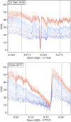 |
Fig. 1 Peak S/N for a single pixel element over time for the first night of observations (top) and the second (bottom), showing all echelle orders. The colour scale represents the wavelength range of the echelle orders from blue to red. The times of ingress and egress are indicated by the black dotted lines. The strong dip in S/N on the first night was caused by loss of guiding: the three exposures affected were removed from our analysis. The S/N of the second night was affected by pointing drift and variable seeing. |
3 Analysis
3.1 Pre-processing steps
We follow a methodology common today in the search for molecular and atomic species in high-resolution spectral time series (Snellen et al. 2010; Brogi et al. 2012; Birkby et al. 2013; Nugroho et al. 2017). The first step is to remove all trends within the data that are static or quasi-static in time, leaving behind – in theory – the Doppler-shifted planetary signal (after removal of its continuum) plus photon noise. An example of our data processing on a single order is shown in Fig. 2.
First, the variation in the blaze function was removed. This was accomplished by dividing each order of time-series spectra by the median spectrum, then smoothing the resulting spectral residuals with a median filter with a width of 15 pixels and a Gaussian filter with a standard deviation of 50 pixels, creating a smoothed map of the blaze distortion per order. The original time-series spectra were then divided through by the blaze distortion map. Instead of removing the blaze function altogether, this placed each spectrum on a “common” blaze. This was done as any common trends in time would be removed later in the pre-processing, and also ensured that spectral information was optimally preserved. The blaze correction was found to be unstable at the blue end of each spectral order, where the S/N was very low: subsequently, the first 500 pixels of each order were removed from our analysis. This removed area represented only 12% of each order of 4096 pixels and lay entirely within the overlapping wavelength region of the echelle orders, so its removal was not expected to be significant.
Next, the quasi-static telluric and stellar spectral features were removed from the time-series using the SYSREM algorithm (Tamuz et al. 2005). First used in this context by Birkby et al. (2013), SYSREM has become a standard tool for the detrending of high-resolution time-series spectra (e.g. Birkby et al. 2017, Nugroho et al. 2017). The main advantage SYSREM retains over other PCA-based detrending methods lies in its inherent treatment of the pixel uncertainties. Rather than simply using Poisson-noise statistics, we estimated the pixel uncertainties by taking an outer product of the time-wise and wavelength-wise variance of each order. This was done due to the removal of the stellar spectrum inherent to the cross-correlation technique. Poisson-noise estimates based on count-rates and read-noise will impose lower uncertainties on negative values of the residuals, causing a bias in the uncertainty determination (Gibson et al. 2020).
We used SYSREM to create 2D model representations of each time-series order as an outer product of two column vectors. This model was then subtracted from the data and the next SYSREM iteration determined from the residuals, which was subtracted again. However, instead of using the resulting iteratively model-subtracted residuals, we instead summed the SYSREM models for each iteration and divided each time-series order by this model. This had the effect of preserving the relative line-strengths of the planet’s transmission spectrum. The detrended residuals were then weighted by the pixeluncertainties, which ensured that noisier, low-flux areas of the time-series contributed less to the analysis.
Finally, the spectra were super-sampled to 2/3 of the average pixel width for each order and corrected to the stellar rest frame in a single linear interpolation, adjusting for both the barycentric velocity variations and the systemic velocity, and the wavelength scale was linearised in Δλ.
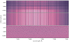 |
Fig. 2 Data-processing steps for a single echelle order. Top: raw extracted time-series spectra after cleaning of outliers. Middle: time-series spectra after blaze-correction. Bottom: detrended residuals from the division of the SYSREM model weighted by the uncertainties. Minor structure remains in the residuals due to lower weighting of low-S/N orders caused by poorer seeing (horizontal banding) and due to imperfect removal of time-dependent tellurics (vertical banding at bottom). The telluric structure does not persist into the in-transit frames and is therefore weighted-out in later analysis. |
3.2 Model transmission spectra
Constraining the existence of molecular or atomic features using the high-resolution cross-correlation technique requires models of the planet’s atmosphere to act as cross-correlation templates. These models are generated using high-temperature line lists for the species of interest to generate absorption cross-sections which can be fed into radiative transfer models to create template spectra for the cross-correlation process. However, the cross-correlation technique is highly sensitive to line position and small inaccuracies in line lists can result in the reduction or non-detection of exoplanetary signals (Hoeijmakers et al. 2015).
Model spectra were generated for TiO and VO using a method similar to that outlined in Nugroho et al. (2020), with planetary and atmospheric parameters taken from Evans et al. (2018) in order to provide the most direct comparison to their transmission spectrum. The full list of system and planetary parameters used in this work is presented in Table 1.
To calculate the cross-section of VO, the EXOMOL line list (McKemmish et al. 2016, Tennyson & Yurchenko 2012) was used. The TiO cross-sections were generated using three different line lists: Plez (1998) in both its original 1998 incarnation and the updated, corrected 2012 version, and the new TOTO line list from EXOMOL (McKemmish et al. 2019). This was done to allow us to benchmark the performance of the different TiO line lists against each other, both in the event of a detection and in our injection tests, as line lists are known to vary considerably. The Plez 2012 and TOTO line lists both explicitly include experimental data: Plez 2012 incorporates experimental line lists and TOTO includes experimentally-derived energy levels. Conversely, the VO line list and Plez 1998 are derived entirely from quantum chemistry calculations and are thus thought to be less accurate and potentially inappropriate for high-resolution cross-correlation. We discuss this issue further in Sect. 4.
For VO, we only considered 51V16O. For TiO, we considered the five most stable isotopologues: 46Ti16O, 47Ti16O, 48Ti16O, 49Ti16O, and 50Ti16O. The cross-section was calculated using HELIOS-K (Grimm & Heng 2015) assuming a Voigt line profile with thermal and natural broadening only at a resolution of 0.01 cm−1 with an absolute line wing cut-off of 100 cm−1.
We produced the transmission spectrum of WASP-121b by assuming a 1D plane-parallel isothermal atmosphere divided into a hundred layers evenly spaced in log pressure from 2 to 10−12 bar. All spectra were generated at four different temperatures of 1500 (consistent with Evans et al. 2018), 2000, 2500, and 3000 K in order to cover the range of potential temperatures at the limb. The scale height was kept fixed at 550 km to provide the best match to the low-resolution transmission spectrum measured by Evans et al. (2018). An example of one of the spectra and its change with temperature is shown in Fig. 3.
For both elements, we assumed a constant volume mixing ratio (VMR) at all pressures, ranging from 10−13 to 10−3. For VO we also assumed a VMR of 10−6.6, consistent with the detection of Evans et al. (2018). We included Rayleigh scattering by H2 and bound-free continuum absorption by H− with a VMR of 5 × 10⁻¹⁰, and set a cloud deck at P = 20 mbar, again to be consistent with Evans et al. (2018). The radius of the planet as a function of wavelength was then calculated by integrating the opacity through transit chords.
Lastly, we removed the continuum and the scattering profile from the model spectra by subtracting a forward-backward Butterworthlow-pass filter to remove any low-frequency structure from the model spectra caused by large areas of densely overlapping lines, as all such structure was removed from our spectra by the pre-processing steps outlined in Sect. 3.1. These low-frequency structures in the models also tended to “catch” any remaining structure in our spectra that had been imperfectly removed by SYSREM, causing spurious artifacts in the cross-correlation.
Stellar and planetary parameters for the WASP-121b system utilised in this paper.
3.3 Cross-correlation
As described in Sect. 3.1, we divided the orders of our spectra through by a SYSREM model consisting of nine iterations to remove the stellar and telluric features. The optimal number of SYSREM iterations was arrived at empirically through injection tests, where the aim was to find the lowest number of SYSREM iterations that would still provide a strong detection of an injected signal. The number of iterations was minimised as, at high numbers of iterations, SYSREM has been found to reduce or remove the exoplanet spectrum (Cabot et al. 2019). Unlike many recent papers utilising the cross-correlation method (e.g. Yan et al. 2019), we did not need to model and remove the stellar spectrum or the Rossiter-McLaughlin effect, as TiO and VO are not expected to exist in the atmosphere of WASP-121, an F6V star. As also mentioned in Sect. 3.1, we further weighted the SYSREM residuals by the pixel variance to ensure that noisier areas of the time-series contributed less to the analysis.
After wavelength linearisation and correction to the stellar rest frame, each frame of each order was then cross-correlated with the corresponding section of the model spectra (also at rest), using the NumPy function numpy.correlate. As no planetary signal was expected in the frames occurring out of transit, and any signal would be weaker during ingress and egress, the resulting time-series of cross-correlation functions was then weighted by a simple transit model for WASP-121b using the equations of Mandel & Agol (2002) and assuming no limb-darkening.
The cross-correlation function is expected to peak where there is a match between the model template and the spectra; this peak, if extant, will be Doppler-shifted over time, resulting in a slanted trace in the cross-correlation time-series. For very strong molecular signals, this trace can be seen with the naked eye (e.g. Snellen et al. 2010). For weaker signals, such as those where the molecules are predicted to be less abundant in the atmosphere, the next step is to integrate the cross-correlation time series over a range of predicted planetary radial velocity semi-amplitudes, where the RV at each frame vp is given by:
![Mathematical equation: \[ v_{\textrm{p}}(\phi) = v_{\textrm{sys}} + K_{\textrm{p}}\sin{(2\pi\phi)}, \]](/articles/aa/full_html/2020/04/aa37409-19/aa37409-19-eq1.png)
where vsys is the systemic velocity, Kp is the radial velocity semi-amplitude of the planet and ϕ is the orbital phase of the planet, where ϕ = 0 represents the mid-transit time. We note that here, vsys is expected to be zero, as the spectra have already been shifted to the stellar rest frame by correcting for both the systemic and the barycentric velocity. The x-axis of the cross-correlation time series can thus be thought of in terms of velocity “lag” from the stellar rest frame.
We integrated the resulting cross-correlation function time-series for each order by interpolating each order time-series to a predicted radial velocity curve using values for Kp from −500 to +500 km s−1 in steps of 1 km s−1, smaller than the average single resolution element of the original spectra (~ 2.5 km s−1). These were then summed column-wise in time and stacked to create a series of cross-correlation velocity heat maps, one for each order, where the y-axis was now Kp and the x-axis, as previously, was in velocity “lag” from the stellar rest frame, or vsys. These individual order maps were then summed together to form a final map. The large range in Kp was chosen in order to create large cross-correlation maps so that the overall noise profile could be studied. Due to the use of the cross-correlation, the z-axis was in arbitrary units: in order to set a detection significance, the maps were divided through by their standard deviation away from the location of the predicted signal. Our detection threshold was set at 4σ due to both our simplistic significance calculation and to the presence of noise fluctuations in the cross-correlation map which can reach this level. As demonstrated in Cabot et al. (2019), these fluctuations can be mistaken for detections if they appear in the expected position.
This process was repeated for every template described in Sect. 3.2 and a cross-correlation map was generated for each template.
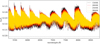 |
Fig. 3 Example model spectrum of TiO with VMR = 10−6 before continuum removal, with all four temperatures overplotted to show the change in relative line strength with temperature. The black dotted line indicates the position of the cloud deck. |
3.4 Results and injection tests
No significant signal was found in any of the cross-correlation maps for TiO or VO at any volume mixing ratio, temperature or line list, whether at the expected value of Kp or otherwise. Examples are shown in the top two rows of Fig. 4.
The possibility remained that this non-detection could be due to the predicted signal being fainter than our ability to retrieve it. To test this hypothesis, we performed a series of injection tests. The model spectra used to attempt to retrieve the signal described in Sect. 3.2 were convolved to the instrumental resolution and multiplied into the original extracted spectra before the pre-processing steps outlined in Sect. 3.1 at a Kp of −217 km s−1, a value chosen to have an identical velocity curve to the expected signal but reversed, to ensure that the injected signal would not be enhanced by any extant, undetected VO or TiO signal. Two of the resultant cross-correlation maps are shown in the bottom row of Fig. 4, for the Evans et al. (2018) log VMR value of −6.6 and a similar log VMR of −7 for TiO, using the 1500 K temperature also inferred by Evans et al. (2018). The injected signal was recovered at 6.9σ for VO and 7.2σ for TiO, demonstrating that were VO present at the abundance and temperature predicted by Evans et al. (2018), our technique would detect it. A slice through the cross-correlation maps of both the non-detections and the injection tests at the expected value of Kp is shown in Fig. 5.
The injection tests were also used to explore rough detection limits for VO and TiO via the injection of templates identical in all parameters but for log VMR of the species in question. The detection threshold was once again set at 4σ for the reasons stated in Sect. 3.3. As shown in Fig. 6, assuming a temperature of 1500 K, by interpolating from our injection tests, we can theoretically detect the presence of VO in the atmosphere of WASP-121b using our technique down to an abundance of log VMR [VO] = −7.9. For TiO, we can theoretically detect its presence down to an abundance of log VMR [TiO] = −9.3, thus placing a detection limit upon TiO lower than the limit of [TiO] < −7.9 placed by Evans et al. (2018). Both of our detection limits are subsolar, where the solar abundance values are −7.1 and −8.0 for TiO and VO, respectively. We also find a reduction in detection significance with temperature for both VO and TiO in our injection tests. As we held scale height constant (at 550 km) in our model spectra in order to match the previously-measured transmission spectrum of Evans et al. (2018), the effect of increasing temperature is to change the relative line strengths of the spectral lines. As can be partially seen in Fig. 3, increasing the temperature had the effect of reducing the strength of many the strongest lines, an effect not quite offset by the strengthening of weaker lines. This led to the overall reduction in detection significance shown in Fig. 6.
However, we note that 550 km is an extremely conservative estimate for the scale height of WASP-121b, based on the limb-averaged temperature of ~1500 K presented in Evans et al. (2018). More recent work has indicated that the limb and nightside temperatures of WASP-121b may be much higher (Bourrier et al. 2020b; Daylan et al. 2019; Gibson et al. 2020), which would result in much larger scale heights: indeed, Gibson et al. (2020) retrieve a scale height of 960 km in their analysis. As a simple test of the effects of increasing scale height, we performed a linear scaling of our models to mimic the effects of increasing the scale height from 550 to 960 km. The results, also presented in Fig. 6, show that increasing the scale height leads to a significant increase in detection significance and a reduction in detection limits. We chose, however, to retain the more conservative estimates gained from the lower estimate of the scale height.
A more robust method of obtaining a detection significance was also tested following Esteves et al. (2017), in which the spectral time-series was shuffled randomly in time and the cross-correlation maps regenerated 1000 times. These maps were then used to set the pixel-by-pixel standard deviation of the original map. However, this method was found to result in similar or higher detection significances than the simpler method outlined in Sect. 3, and we have therefore adopted the more conservative estimates from the initial method.
Caution should be applied in interpreting the results of these injection tests. Firstly, the injected signal is identical to the template used to retrieve it, which will artificially boost the detection signal, though this is not expected to do so dramatically. Secondly, there is a known degeneracy between chemical abundances and the scattering properties of the atmosphere (Benneke & Seager 2012; Heng & Kitzmann 2017). For our injected spectral models, we have assumed a cloud deck at 20 mbar and a H− VMR of 5 × 10⁻¹⁰, consistent with Evans et al. (2018), and our detection limits should be considered in this context. Finally, the VO line list is known to be unsuitable for high-resolution cross-correlation. We discuss this further in Sect. 4.
We also present the results of injection tests using differing TiO line lists in Fig. 7. While all line lists follow the same overalltrend, they can be seen to behave differently. In the case of ToTo, the increased number of lines present in the line list is likely to be the cause of the improvement in the signal recovery. For Plez 2012, the corrections made using laboratory measurements of 48Ti16O increase the line strength of some of the stronger lines, again boosting signal recovery.
Additionally, we investigated the behaviour of the recovered detection signal when injecting models created with one line list and retrieving with models using another. Due to the small variations in line strengths and positions between different line lists, this simple test serves as an indication of the effects of using inaccurate line lists in high-resolution cross-correlation. Further in-depth analysis of a range of TiO line lists and their effects upon signal retrieval in the cross-correlation process will be presented inNugroho et al. (in prep).
The results are presented in Fig. 7. Injecting the ToTo model and retrieving with Plez 2012 results in values for the detection significance which do not rise above our chosen threshold of 4σ at any log VMR: the differences between the two line lists have caused the injected signal to become essentially undetectable. However, when performing the inverse of this test, injecting models using the Plez 2012 line list and retrieving using ToTo, the detection significance rises once again. Though it does not reach the ~ 7σ level of tests using the same models for both injection and retrieval, it still results in detectable signals for a similar range of log VMR.
The underlying cause for this difference may be due to the greater number of lines in the ToTo line list. The densely-overlapping lines form a pseudo-continuum in the models, which weakens overall line contrast. When cross-correlating using ToTo models, the greater number of lines mitigates this effect: when attempting retrieval using Plez 2012, which has less lines overall, the effect is enhanced, and the signal is no longer well-recovered. This test emphasises the importance of understanding the effects inaccurate line lists can have on signal retrieval using the cross-correlation methodology; we discuss this further in Sect. 4.
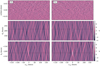 |
Fig. 4 Results from cross-correlation with VO (left) and TiO (right) templates, at a log VMR of −6.6 and −7 respectively, for 1500 K. Top row: cross-correlation function time series summed over all echelle orders, showing no visible trace. Middle: cross-correlation maps summed over all echelle orders, showing non-detections for both species: the black dotted lines indicate the expected velocity position for the signal (Kp = 217 km s−1). Bottom: results from injection tests, showing a detection of the injected signal at 6.9σ for VO and 7.2σ for TiO at the expected velocity position. We note that the expected value for vsys is zero as the spectra have been corrected to the stellar rest frame. |
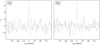 |
Fig. 5 Slices taken from the cross-correlation maps in Fig. 4 at Kp = ±217 km s−1, with the non-detection in blue and the injection test in orange for comparison. |
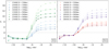 |
Fig. 6 Detection significance vs. log volume mixing ratio abundance of VO (left) and TiO (right) from signal injection tests for all four temperatures considered. Two scale heights of 550 and 960 km were tested for all temperatures. The black dotted line indicates the chosen detection threshold of 4σ. |
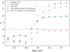 |
Fig. 7 Detection significance vs. log volume mixing ratio abundance of TiO for injection tests using three different line lists, including the results of injecting one line list and retrievingwith another. The black dotted line indicates the chosen detection threshold of 4σ. |
4 Discussion
Our results show non-detections of TiO and VO in the atmosphere of WASP-121b using the standard cross-correlation methodology. Additionally, our injection tests show that if VO were present at the super-solar abundances predicted in Evans et al. (2018) or Mikal-Evans et al. (2019), we would detect the subsequent molecular signal at a high significance. Doubt had already been placed upon the existence of TiO in the limb of WASP-121b by Evans et al. (2018), who fit their transmission spectra best with a model containing VO only; the emission spectra presented in Evans et al. (2017) and Mikal-Evans et al. (2019) is similarly best fit by models containing only VO. Our non-detection of TiO is thus consistent with previous results and adds further evidence to the non-existence of TiO in detectable quantities in the atmosphere of WASP-121b.
Conversely, our non-detection of VO contradicts results presented in Evans et al. (2016, 2017, 2018) and Mikal-Evans et al. (2019), who find evidence for VO in both emission and transmission at low-resolution. It is known that low-resolution spectroscopy is troubled by the imperfect removal of systematics, especially shown in the case of STIS on HST (Gibson et al. 2017, 2019), the instrument used for the transmission spectrum presented in Evans et al. (2018). The effects of systematics on low-resolution spectra can also be seen in the improved retrieval analysis of the emission spectrum presented in Mikal-Evans et al. (2019) using WFC3 on HST. Here, they no longer fit a strong feature at 1.2 μm attributed to VO in Evans et al. (2017): the 1.2 μm feature is now thus suspected to be an imperfectly-removed systematic. However, although in all cases their evidence for VO is inferred from best-fit models rather than a direct detection, models containing VO are best-fit in both transmission and emission, using two separate instruments. In the face of this strong evidence for the presence of VO, our non-detection seems puzzling.
However, a major question remains about the suitability of the VO line list for high-resolution spectroscopy in the detection of exoplanet atmospheres. The recent release of the EXOMOL group’s TOTO line list for TiO (McKemmish et al. 2019) provided the exoplanet community with a TiO line list accurate enough at high temperatures to be used with the cross-correlation technique, after previous attempts showed that many of the current line lists were insufficient for this task (Hoeijmakers et al. 2015). Their MARVEL codebase uses laboratory measurements to correct and refine the quantum chemistry calculations used to generate the line lists, theoretically resulting in more accurate results (McKemmish et al. 2017). The “MARVEL-ised” TOTO line list has been found to perform slightly better than other line lists in cross-correlation with M-dwarf stars (McKemmish et al. 2019). However, the VO line list has not yet been similarly corrected. As a result, the EXOMOL team caution that the VO line list used in this paper is probably not accurate enough for high-resolution spectroscopic exploration of exoplanet atmospheres (Sergey Yurchenko, priv. comm.). Until a more accurate high-temperature line list for VO is calculated, it is impossible to state whether our non-detection is due to the true absence of gaseous VO in the limb of WASP-121b or due to an inaccurate line list weakening the strength of the recovered signal. Indeed, our own injection tests presented in Sect. 3.4, in which we inject models created with one line list and attempt retrieval using another in order to mimic the effects of using inaccurate line lists, show drastic changes in signal detection and significance depending on which line lists are used. Our results concerning VO should thus be interpreted in this context.
We also performed a number of injection tests in order to set a rough detection limit on the presence of VO and TiO, in which we ruled out the presence of VO and TiO at abundances greater than −7.88 and −8.18 log VMR respectively at a temperature of 1500 K. However, these figures all assume a cloud deck placed at a constant pressure of 20 mbar and a H− VMR of 5 × 10⁻¹⁰. There is a well-known degeneracy between abundance and scattering properties, where the presence of clouds and hazes can mute spectral features such that a given spectral signal can be produced byeither a low fractional abundance of the species in a clear atmosphere or a higher fractional abundance in the presence of clouds and hazes (Benneke & Seager 2012; Heng & Kitzmann 2017). Since our method removes both the continuum and the scattering profile from our spectra, we are unable to make any measurements which could break the degeneracy. This indicates that we cannot place too much weight upon these detection limits as absolute figures but rather that they should be examined in the context of the strength of the lines appearing above the continuum. Our upper limits for both TiO and VO correspond to a line strength for the strongest lines in the template of ~ 0.014 ΔF.
If we momentarily set aside concerns regarding the accuracy of the VO line list, the non-detection of TiO and VO could be caused by several factors. First, it should be noted that our spectral models (see Sect. 3.2) assume a well-mixed atmosphere. Atmospheric retrievals (e.g. Daylan et al. 2019; Mikal-Evans et al. 2019) show that the abundances of TiO and VO are expected to vary greatly with altitude. In the case of a very hot thermosphere (>3000 K), TiO and VO would be dissociated at high altitude, causing a truncation of the lines present in the transmission spectrum over the altitude range probed by high-resolution spectroscopy. This could potentially cause a dilution in signal that could lead to a non-detection. Further work could focus on the injection of more sophisticated spectral models where molecular abundance varies with pressure to test whether high-altitude dissociation is strong enough to remove the possibility of detection altogether.
It has been suggested that gravitational settling could drag TiO and VO down from the upper atmosphere to the colder layer in the deeper atmosphere, where it subsequently condenses. Alternatively, the cooler temperatures on the night-side could cause TiO and VO to condense out (primarily into Ti3 O5 and V2 O3), and due to the high-speed winds from day- to night-side expected in tidally-locked hot Jupiters, these condensed molecules are not efficiently redistributed to the hot day-side. Thus, Ti and V remain locked in condensed form (the cold-trapping effect: Hubeny et al. 2003; Spiegel et al. 2009; Parmentier et al. 2013, 2016; Beatty et al. 2017). However, the detection of Fe and Mg (Sing et al. 2019; Gibson et al. 2020; Bourrier et al. 2020a; Cabot et al. 2020) in the atmosphere of WASP-121b suggests that cold-trapping does not play a large role, as we would expect Fe and Mg to be cold-trapped as well.
Additionally, calculations from TESS phase curve measurements made by Bourrier et al. (2020b) and Daylan et al. (2019) indicate a nightside temperature for WASP-121b of 2190 K, higher than the condensation temperatures of TiO and VO, although their observations probe high in the atmosphere (1–10 mbar) and do not rule out the possibility of cold-trapping at lower altitudes.
Parmentier et al. (2018) predicted that TiO and VO may, in the case of WASP-121b, be thermally dissociated in the dayside atmosphere; the detection of these molecules in the terminator during transmission would thus depend on their recombination timescales compared to the atmospheric recirculation timescale. However, a recent work using the blue arm of the data presented in this paper by Gibson et al. (2020) retrieves a high limb temperature of ≳ 3000 K, albeit using simplified isothermal models. When considered in the context of the atmospheric retrievals of Daylan et al. (2019), this temperature would cause the dissociation of TiO and VO in the limb even at the lower altitudes probed by our data, reducing the log VMR of both species to < −10, well below the detection limits we set with our injection tests.
It is also interesting to note that the work of Evans et al. (2017, 2018) and Mikal-Evans et al. (2019) infers the presence of VO, but not TiO, when both were predicted as inversion-drivers by Hubeny et al. (2003) and Fortney et al. (2008) and were largely expected to occur together. It has been shown in the models of Goyal et al. (2019) that greater abundance of VO over TiO is only expected in a very narrow temperature range: ~ 1700–1800 K assuming rainout condensation, or ~1200–1400 K assuming local condensation. This highlights the importance of robust detections and non-detections of TiO and VO as a diagnostic for temperature and condensation processes in the atmospheres of ultra-hot Jupiters.
Despite our non-detection of TiO and VO, Evans et al. (2018) still show a feature in their transmission spectra at 600–800 nm consistent with the presence of VO (or perhaps another molecule absorbing strongly in this range). Additionally, their emission spectra (Evans et al. 2017; Mikal-Evans et al. 2019) are still best-fit with models containing VO and clearly show water emission features consistent with the presence of a temperature inversion. It was theorised by Spiegel et al. (2009) that a hot Jupiter witha solar carbon-to-oxygen ratio would require TiO of at least solar abundance to cause a temperature inversion, a level which both we and Evans et al. (2018) rule out in our analysis. Our analysis in this paper now seems to rule out the presence of VO also, although again we emphasise that VO cannot be robustly ruled out using high-resolution cross-correlation methodology until a more suitably accurate line list is published. Nevertheless, although TiO and VO were long thought to be the predominant cause of temperature inversions in hot Jupiters, it may now be time to look for other culprits.
Recent theoretical work has postulated a range of potential optical absorbers such as SiO, Fe, Mg, AlO, CaO and metal hydrides (Lothringer et al. 2018; Lothringer & Barman 2019; Gandhi & Madhusudhan 2019), some of which (such as AlO) have absorption bands in the 600–800 nm range. Gandhi & Madhusudhan (2019) also suggested a theoretical link between the C/O ratio and the presence of a temperature inversion, postulating that a reduced infrared opacity due to a low H2 O abundance in WASP-121b could contribute towards the existence of an inversion layer; the presence of H2 O emission features, however, would appear to rule out this possibility. Finally, the transmission spectrum presented by Evans et al. (2018) shows a strong upward trend in the blue optical much steeper than would be consistent with Rayleigh scattering, which they tentatively identify as due to the presence of SH, another molecule known to absorb strongly in the optical and thus theoreticallycontribute to an inversion layer (Zahnle et al. 2009). However, this slope could also be attributed to a forest of atomic metal lines. Indeed, a recent analysis by our group of the blue arm of the UVES data used in this paper (Gibson et al. 2020) found strong evidence for the presence of Fe I in the atmosphere of WASP-121b, a discovery supported by recent analyses of HARPS high-resolution spectra by Bourrier et al. (2020a) and Cabot et al. (2020). Fe I has strong absorption at blue-optical wavelengths, and as WASP-121 is an F6-type star, this could lead to significant amounts of energy being deposited at high altitudes and could potentially be the sole or predominant cause of the observed temperature inversion. However, Fe I cannot be responsible for the absorption feature seen in the transmission spectra at 600–800 nm in the transmission spectrum of Evans et al. (2018) and if it is not caused by VO, the presence of another optical absorber with strong absorption in this range cannot be ruled out.
Future searches could focus on the detection of a molecular species with strong absorption features in this range, such as AlO and MgH, in order to constrain the origin of this feature. Indeed, a tentative detection of AlO has already been reported in the atmosphere of ultra-hot WASP-33b (von Essen et al. 2019), indicating that this may be a productive avenue of inquiry. Alternatively, should a more robust line list for VO be produced, a reanalysis of the data presented in this work could more definitively confirm or rule out the presence of VO in WASP-121b.
5 Conclusions
We present a non-detection of TiO and VO in the atmosphere of the ultra-hot Jupiter WASP-121b, a planet previously shown to have evidence for a temperature inversion and for the existence of VO (but not necessarily TiO). Using injection tests, we show that were VO present in the abundance predicted by Evans et al. (2018), we were able to retrieve the molecular signal using our technique with relative ease. Additionally, we place rough constraints on the presence of VO in the limb of WASP-121b using injection tests and we find that – while bearing in mind the established degeneracy between scattering properties and abundance – we can detect the presence of VO down to a sub-solar log volume mixing ratio of −7.88, and TiO down to a sub-solar log volume mixing ratio of −9.26. The absence of TiO and VO in transmission could be due to thermal dissociation of these molecules on the hot dayside of WASP-121b in conjunction with a slow recombination timescale, or due to cold-trapping locking condensed TiO and VO on the colder nightside. However, we also emphasise that the VO line list utilised for this paper is thought to lack the accuracy in line position required for high-resolution spectroscopic searches for molecular species. Despite the strength of our detection in our injection tests, it is nevertheless clear that a definitive answer on the existence of VO in the limb of WASP-121b using high-resolution spectroscopy will be dependent on a more accurate, updated line list for VO.
Recent work from our team (Gibson et al. 2020) posits a different source species (Fe I) for the observed temperature inversion in WASP-121b: however, Fe I cannot be responsible for the observed absorption feature at 600–800 nm in the transmission spectrum presented by Evans et al. (2018). If it is physical, and not caused by the presence of VO, a range of molecular species could be responsible for this feature, and future work will focus on the search for these and for many other such molecules theorised to be present in the atmospheres of ultra-hot Jupiters.
Acknowledgements
The authors are very grateful to the anonymous referee for their insightful comments and suggestions. This work is based on observations collected at the European Organisation for Astronomical Research in the Southern Hemisphere under ESO programme 098.C-0547. S.R.M. acknowledges funding from the Northern Ireland Department for the Economy. N.P.G. gratefully acknowledges support from Science Foundation Ireland and the Royal Society in the form of a University Research Fellowship. S.K.N. and C.A.W. would like to acknowledge support from UK Science Technology and Facility Council grant ST/P000312/1. We are exceptionally grateful to the developers of the NUMPY, SCIPY, MATPLOTLIB, IPYTHON, SCIKIT-LEARN and ASTROPY packages, which were used extensively in this work (van der Walt et al. 2011; Virtanen et al. 2019; Hunter 2007; Perez & Granger 2007; Pedregosa et al. 2011; Astropy Collaboration 2013). The perceptually-uniform scientific colour map used in Figs. 2 and 4 is Acton by Crameri (2018).
References
- Arcangeli, J., Désert, J.-M., Line, M. R., et al. 2018, ApJ, 855, L30 [NASA ADS] [CrossRef] [Google Scholar]
- Astropy Collaboration (Robitaille, T. P., et al.) 2013, A&A, 558, A33 [NASA ADS] [CrossRef] [EDP Sciences] [Google Scholar]
- Bean, J. L., Miller-Ricci Kempton, E., & Homeier, D. 2010, Nature, 468, 669 [NASA ADS] [CrossRef] [PubMed] [Google Scholar]
- Bean, J. L., Désert, J.-M., Kabath, P., et al. 2011, ApJ, 743, 92 [NASA ADS] [CrossRef] [Google Scholar]
- Beatty, T. G., Madhusudhan, N., Tsiaras, A., et al. 2017, AJ, 154, 158 [NASA ADS] [CrossRef] [Google Scholar]
- Benneke, B., & Seager, S. 2012, ApJ, 753, 100 [NASA ADS] [CrossRef] [Google Scholar]
- Berta, Z. K., Charbonneau, D., Désert, J.-M., et al. 2012, ApJ, 747, 35 [NASA ADS] [CrossRef] [Google Scholar]
- Birkby, J. L., de Kok, R. J., Brogi, M., et al. 2013, MNRAS, 436, L35 [NASA ADS] [CrossRef] [Google Scholar]
- Birkby, J. L., de Kok, R. J., Brogi, M., Schwarz, H., & Snellen, I. A. G. 2017, AJ, 153, 138 [NASA ADS] [CrossRef] [Google Scholar]
- Bourrier, V., Ehrenreich, D., Lendl, M., et al. 2020a, A&A, 635, A205 [NASA ADS] [CrossRef] [EDP Sciences] [Google Scholar]
- Bourrier, V., Kitzmann, D., Kuntzer, T., et al. 2020b, A&A, in press, https://doi.org/10.1051/0004-6361/201936647 [Google Scholar]
- Brogi, M., Snellen, I. A. G., de Kok, R. J., et al. 2012, Nature, 486, 502 [NASA ADS] [CrossRef] [PubMed] [Google Scholar]
- Brogi, M., de Kok, R. J., Birkby, J. L., Schwarz, H., & Snellen, I. A. G. 2014, A&A, 565, A124 [NASA ADS] [CrossRef] [EDP Sciences] [Google Scholar]
- Brogi, M., de Kok, R. J., Albrecht, S., et al. 2016, ApJ, 817, 106 [NASA ADS] [CrossRef] [Google Scholar]
- Brown, T. M. 2001, ApJ, 553, 1006 [NASA ADS] [CrossRef] [Google Scholar]
- Cabot, S. H. C., Madhusudhan, N., Hawker, G. A., & Gandhi, S. 2019, MNRAS, 482, 4422 [NASA ADS] [CrossRef] [Google Scholar]
- Cabot, S. H. C., Madhusudhan, N., Welbanks, L., Piette, A., & Gandhi, S. 2020, MNRAS, 494, 363 [NASA ADS] [CrossRef] [Google Scholar]
- Cartier, K. M. S., Beatty, T. G., Zhao, M., et al. 2017, AJ, 153, 34 [NASA ADS] [CrossRef] [Google Scholar]
- Charbonneau, D., Brown, T. M., Noyes, R. W., & Gilliland, R. L. 2002, ApJ, 568, 377 [NASA ADS] [CrossRef] [Google Scholar]
- Crameri, F. 2018, Scientific colour maps [Google Scholar]
- Crossfield, I. J. M., Barman, T., Hansen, B. M. S., & Howard, A. W. 2013, A&A, 559, A33 [NASA ADS] [CrossRef] [EDP Sciences] [Google Scholar]
- Czesla, S., Klocová, T., Khalafinejad, S., Wolter, U., & Schmitt, J. H. M. M. 2015, A&A, 582, A51 [NASA ADS] [CrossRef] [EDP Sciences] [Google Scholar]
- Daylan, T., Günther, M. N., Mikal-Evans, T., et al. 2019, ArXiv e-prints, [arXiv:1909.03000] [Google Scholar]
- Dekker, H., D’Odorico, S., Kaufer, A., Delabre, B., & Kotzlowski, H. 2000, SPIE Conf. Ser., 4008, 534 [Google Scholar]
- Delrez, L., Santerne, A., Almenara, J. M., et al. 2016, MNRAS, 458, 4025 [NASA ADS] [CrossRef] [Google Scholar]
- Diamond-Lowe, H., Stevenson, K. B., Bean, J. L., Line, M. R., & Fortney, J. J. 2014, ApJ, 796, 66 [NASA ADS] [CrossRef] [Google Scholar]
- Espinoza, N., Rackham, B. V., Jordán, A., et al. 2019, MNRAS, 482, 2065 [Google Scholar]
- Esteves, L. J., de Mooij, E. J. W., Jayawardhana, R., Watson, C., & de Kok, R. 2017, AJ, 153, 268 [NASA ADS] [CrossRef] [Google Scholar]
- Evans, T. M., Aigrain, S., Gibson, N., et al. 2015, MNRAS, 451, 680 [NASA ADS] [CrossRef] [Google Scholar]
- Evans, T. M., Sing, D. K., Wakeford, H. R., et al. 2016, ApJ, 822, L4 [NASA ADS] [CrossRef] [Google Scholar]
- Evans, T. M., Sing, D. K., Kataria, T., et al. 2017, Nature, 548, 58 [NASA ADS] [CrossRef] [Google Scholar]
- Evans, T. M., Sing, D. K., Goyal, J. M., et al. 2018, AJ, 156, 283 [NASA ADS] [CrossRef] [Google Scholar]
- Fortney, J. J., Lodders, K., Marley, M. S., & Freedman, R. S. 2008, ApJ, 678, 1419 [NASA ADS] [CrossRef] [Google Scholar]
- Gaia Collaboration 2018, VizieR Online Data Catalog: I/345 [Google Scholar]
- Gandhi, S., & Madhusudhan, N. 2019, MNRAS, 485, 5817 [NASA ADS] [CrossRef] [Google Scholar]
- Gibson, N. P., Aigrain, S., Barstow, J. K., et al. 2013a, MNRAS, 428, 3680 [NASA ADS] [CrossRef] [Google Scholar]
- Gibson, N. P., Aigrain, S., Barstow, J. K., et al. 2013b, MNRAS, 436, 2974 [NASA ADS] [CrossRef] [Google Scholar]
- Gibson, N. P., Nikolov, N., Sing, D. K., et al. 2017, MNRAS, 467, 4591 [NASA ADS] [CrossRef] [Google Scholar]
- Gibson, N. P., de Mooij, E. J. W., Evans, T. M., et al. 2019, MNRAS, 482, 606 [NASA ADS] [CrossRef] [Google Scholar]
- Gibson, N. P., Merritt, S., Nugroho, S. K., et al. 2020, MNRAS, 493, 2215 [NASA ADS] [CrossRef] [Google Scholar]
- Goyal, J. M., Wakeford, H. R., Mayne, N. J., et al. 2019, MNRAS, 482, 4503 [NASA ADS] [CrossRef] [Google Scholar]
- Grimm, S. L., & Heng, K. 2015, ApJ, 808, 182 [NASA ADS] [CrossRef] [Google Scholar]
- Guilluy, G., Sozzetti, A., Brogi, M., et al. 2019, A&A, 625, A107 [NASA ADS] [CrossRef] [EDP Sciences] [Google Scholar]
- Hansen, C. J., Schwartz, J. C., & Cowan, N. B. 2014, MNRAS, 444, 3632 [NASA ADS] [CrossRef] [Google Scholar]
- Haynes, K., Mandell, A. M., Madhusudhan, N., Deming, D., & Knutson, H. 2015, ApJ, 806, 146 [NASA ADS] [CrossRef] [Google Scholar]
- Heng, K., & Kitzmann, D. 2017, MNRAS, 470, 2972 [NASA ADS] [CrossRef] [Google Scholar]
- Hoeijmakers, H. J., de Kok, R. J., Snellen, I. A. G., et al. 2015, A&A, 575, A20 [NASA ADS] [CrossRef] [EDP Sciences] [Google Scholar]
- Hoeijmakers, H. J., Ehrenreich, D., Heng, K., et al. 2018, Nature, 560, 453 [NASA ADS] [CrossRef] [Google Scholar]
- Hoeijmakers, H. J., Ehrenreich, D., Kitzmann, D., et al. 2019, A&A, 627, A165 [NASA ADS] [CrossRef] [EDP Sciences] [Google Scholar]
- Høg, E., Fabricius, C., Makarov, V. V., et al. 2000, A&A, 355, L27 [Google Scholar]
- Hubeny, I., Burrows, A., & Sudarsky, D. 2003, ApJ, 594, 1011 [NASA ADS] [CrossRef] [Google Scholar]
- Huitson, C. M., Sing, D. K., Vidal-Madjar, A., et al. 2012, MNRAS, 422, 2477 [NASA ADS] [CrossRef] [Google Scholar]
- Huitson, C. M., Sing, D. K., Pont, F., et al. 2013, MNRAS, 434, 3252 [NASA ADS] [CrossRef] [Google Scholar]
- Hunter, J. D. 2007, Comput. Sci. Eng., 9, 90 [NASA ADS] [CrossRef] [Google Scholar]
- Jordán, A., Espinoza, N., Rabus, M., et al. 2013, ApJ, 778, 184 [NASA ADS] [CrossRef] [Google Scholar]
- Khalafinejad, S., von Essen, C., Hoeijmakers, H. J., et al. 2017, A&A, 598, A131 [NASA ADS] [CrossRef] [EDP Sciences] [Google Scholar]
- Knutson, H. A., Charbonneau, D., Allen, L. E., Burrows, A., & Megeath, S. T. 2008, ApJ, 673, 526 [NASA ADS] [CrossRef] [Google Scholar]
- Kreidberg, L., Bean, J. L., Désert, J.-M., et al. 2014, Nature, 505, 69 [NASA ADS] [CrossRef] [Google Scholar]
- Kreidberg, L., Line, M. R., Parmentier, V., et al. 2018, AJ, 156, 17 [NASA ADS] [CrossRef] [Google Scholar]
- Lendl, M., Delrez, L., Gillon, M., et al. 2016, A&A, 587, A67 [NASA ADS] [CrossRef] [EDP Sciences] [Google Scholar]
- Line, M. R., Stevenson, K. B., Bean, J., et al. 2016, AJ, 152, 203 [NASA ADS] [CrossRef] [Google Scholar]
- Lockwood, A. C., Johnson, J. A., Bender, C. F., et al. 2014, ApJ, 783, L29 [NASA ADS] [CrossRef] [Google Scholar]
- Lothringer, J. D., & Barman, T. 2019, ApJ, 876, 69 [NASA ADS] [CrossRef] [Google Scholar]
- Lothringer, J. D., Barman, T., & Koskinen, T. 2018, ApJ, 866, 27 [NASA ADS] [CrossRef] [Google Scholar]
- Mallonn, M., & Strassmeier, K. G. 2016, A&A, 590, A100 [NASA ADS] [CrossRef] [EDP Sciences] [Google Scholar]
- Mallonn, M., Köhler, J., Alexoudi, X., et al. 2019, A&A, 624, A62 [NASA ADS] [CrossRef] [EDP Sciences] [Google Scholar]
- Mandel, K., & Agol, E. 2002, ApJ, 580, L171 [NASA ADS] [CrossRef] [Google Scholar]
- Mansfield, M., Bean, J. L., Line, M. R., et al. 2018, AJ, 156, 10 [NASA ADS] [CrossRef] [Google Scholar]
- McKemmish, L. K., Yurchenko, S. N., & Tennyson, J. 2016, MNRAS, 463, 771 [NASA ADS] [CrossRef] [Google Scholar]
- McKemmish, L. K., Masseron, T., Sheppard, S., et al. 2017, ApJS, 228, 15 [NASA ADS] [CrossRef] [Google Scholar]
- McKemmish, L. K., Masseron, T., Hoeijmakers, H. J., et al. 2019, MNRAS, 488, 2836 [NASA ADS] [CrossRef] [Google Scholar]
- Mikal-Evans, T., Sing, D. K., Goyal, J. M., et al. 2019, MNRAS, 488, 2222 [NASA ADS] [CrossRef] [Google Scholar]
- Nikolov, N., Sing, D. K., Burrows, A. S., et al. 2015, MNRAS, 447, 463 [NASA ADS] [CrossRef] [Google Scholar]
- Nikolov, N., Sing, D. K., Gibson, N. P., et al. 2016, ApJ, 832, 191 [NASA ADS] [CrossRef] [Google Scholar]
- Nikolov, N., Sing, D. K., Fortney, J. J., et al. 2018, Nature, 557, 526 [NASA ADS] [CrossRef] [Google Scholar]
- Nugroho, S. K., Kawahara, H., Masuda, K., et al. 2017, AJ, 154, 221 [NASA ADS] [CrossRef] [Google Scholar]
- Nugroho, S. K., Gibson, N. P., de Mooij, E. J. W., et al. 2020, MNRAS, submitted [arXiv:2003.04856] [Google Scholar]
- Parmentier, V., Showman, A. P., & Lian, Y. 2013, A&A, 558, A91 [NASA ADS] [CrossRef] [EDP Sciences] [Google Scholar]
- Parmentier, V., Fortney, J. J., Showman, A. P., Morley, C., & Marley, M. S. 2016, ApJ, 828, 22 [NASA ADS] [CrossRef] [Google Scholar]
- Parmentier, V., Line, M. R., Bean, J. L., et al. 2018, A&A, 617, A110 [NASA ADS] [CrossRef] [EDP Sciences] [Google Scholar]
- Pedregosa, F., Varoquaux, G., Gramfort, A., et al. 2011, J. Mach. Learn. Res., 12, 2825 [Google Scholar]
- Perez, F., & Granger, B. E. 2007, Comput. Sci. Eng., 9, 21 [Google Scholar]
- Plez, B. 1998, A&A, 337, 495 [NASA ADS] [Google Scholar]
- Pont, F., Knutson, H., Gilliland, R. L., Moutou, C., & Charbonneau, D. 2008, MNRAS, 385, 109 [NASA ADS] [CrossRef] [Google Scholar]
- Pont, F., Sing, D. K., Gibson, N. P., et al. 2013, MNRAS, 432, 2917 [NASA ADS] [CrossRef] [Google Scholar]
- Salz, M., Schneider, P. C., Fossati, L., et al. 2019, A&A, 623, A57 [NASA ADS] [CrossRef] [EDP Sciences] [Google Scholar]
- Schwarz, H., Brogi, M., de Kok, R., Birkby, J., & Snellen, I. 2015, A&A, 576, A111 [NASA ADS] [CrossRef] [EDP Sciences] [Google Scholar]
- Seager, S., & Sasselov, D. D. 2000, ApJ, 537, 916 [NASA ADS] [CrossRef] [Google Scholar]
- Sedaghati, E., Boffin, H. M. J., MacDonald, R. J., et al. 2017, Nature, 549, 238 [NASA ADS] [CrossRef] [Google Scholar]
- Sing, D. K., Fortney, J. J., Nikolov, N., et al. 2016, Nature, 529, 59 [NASA ADS] [CrossRef] [Google Scholar]
- Sing, D. K., Lavvas, P., Ballester, G. E., et al. 2019, AJ, 158, 91 [NASA ADS] [CrossRef] [Google Scholar]
- Snellen, I. A. G. 2004, MNRAS, 353, L1 [NASA ADS] [CrossRef] [Google Scholar]
- Snellen, I. A. G., de Kok, R. J., de Mooij, E. J. W., & Albrecht, S. 2010, Nature, 465, 1049 [NASA ADS] [CrossRef] [PubMed] [Google Scholar]
- Snellen, I. A. G., Brandl, B. R., de Kok, R. J., et al. 2014, Nature, 509, 63 [NASA ADS] [CrossRef] [Google Scholar]
- Spiegel, D. S., Silverio, K., & Burrows, A. 2009, ApJ, 699, 1487 [NASA ADS] [CrossRef] [Google Scholar]
- Stevenson, K. B., Bean, J. L., Seifahrt, A., et al. 2014, AJ, 147, 161 [NASA ADS] [CrossRef] [Google Scholar]
- Swain, M., Deroo, P., Tinetti, G., et al. 2013, Icarus, 225, 432 [NASA ADS] [CrossRef] [Google Scholar]
- Tamuz, O., Mazeh, T., & Zucker, S. 2005, MNRAS, 356, 1466 [NASA ADS] [CrossRef] [Google Scholar]
- Tennyson, J., & Yurchenko, S. N. 2012, MNRAS, 425, 21 [Google Scholar]
- Tsiaras, A., Waldmann, I. P., Zingales, T., et al. 2018, AJ, 155, 156 [NASA ADS] [CrossRef] [Google Scholar]
- Turner, J. D., de Mooij, E. J. W., Jayawardhana, R., et al. 2020, ApJ, 888, L13 [NASA ADS] [CrossRef] [Google Scholar]
- van der Walt, S., Colbert, S. C., & Varoquaux, G. 2011, Comput. Sci. Eng., 13, 22 [Google Scholar]
- Virtanen, P., Gommers, R., Oliphant, T. E., et al. 2019, ArXiv e-prints, [arXiv:1907.10121] [Google Scholar]
- von Essen, C., Mallonn, M., Welbanks, L., et al. 2019, A&A, 622, A71 [NASA ADS] [CrossRef] [EDP Sciences] [Google Scholar]
- Yan, F., Casasayas-Barris, N., Molaverdikhani, K., et al. 2019, A&A, 632, A69 [NASA ADS] [CrossRef] [EDP Sciences] [Google Scholar]
- Zahnle, K., Marley, M. S., Freedman, R. S., Lodders, K., & Fortney, J. J. 2009, ApJ, 701, L20 [NASA ADS] [CrossRef] [Google Scholar]
- Zellem, R. T., Lewis, N. K., Knutson, H. A., et al. 2014, ApJ, 790, 53 [NASA ADS] [CrossRef] [EDP Sciences] [Google Scholar]
All Tables
Stellar and planetary parameters for the WASP-121b system utilised in this paper.
All Figures
|
Fig. 1 Peak S/N for a single pixel element over time for the first night of observations (top) and the second (bottom), showing all echelle orders. The colour scale represents the wavelength range of the echelle orders from blue to red. The times of ingress and egress are indicated by the black dotted lines. The strong dip in S/N on the first night was caused by loss of guiding: the three exposures affected were removed from our analysis. The S/N of the second night was affected by pointing drift and variable seeing. |
| In the text | |
|
Fig. 2 Data-processing steps for a single echelle order. Top: raw extracted time-series spectra after cleaning of outliers. Middle: time-series spectra after blaze-correction. Bottom: detrended residuals from the division of the SYSREM model weighted by the uncertainties. Minor structure remains in the residuals due to lower weighting of low-S/N orders caused by poorer seeing (horizontal banding) and due to imperfect removal of time-dependent tellurics (vertical banding at bottom). The telluric structure does not persist into the in-transit frames and is therefore weighted-out in later analysis. |
| In the text | |
|
Fig. 3 Example model spectrum of TiO with VMR = 10−6 before continuum removal, with all four temperatures overplotted to show the change in relative line strength with temperature. The black dotted line indicates the position of the cloud deck. |
| In the text | |
|
Fig. 4 Results from cross-correlation with VO (left) and TiO (right) templates, at a log VMR of −6.6 and −7 respectively, for 1500 K. Top row: cross-correlation function time series summed over all echelle orders, showing no visible trace. Middle: cross-correlation maps summed over all echelle orders, showing non-detections for both species: the black dotted lines indicate the expected velocity position for the signal (Kp = 217 km s−1). Bottom: results from injection tests, showing a detection of the injected signal at 6.9σ for VO and 7.2σ for TiO at the expected velocity position. We note that the expected value for vsys is zero as the spectra have been corrected to the stellar rest frame. |
| In the text | |
|
Fig. 5 Slices taken from the cross-correlation maps in Fig. 4 at Kp = ±217 km s−1, with the non-detection in blue and the injection test in orange for comparison. |
| In the text | |
|
Fig. 6 Detection significance vs. log volume mixing ratio abundance of VO (left) and TiO (right) from signal injection tests for all four temperatures considered. Two scale heights of 550 and 960 km were tested for all temperatures. The black dotted line indicates the chosen detection threshold of 4σ. |
| In the text | |
|
Fig. 7 Detection significance vs. log volume mixing ratio abundance of TiO for injection tests using three different line lists, including the results of injecting one line list and retrievingwith another. The black dotted line indicates the chosen detection threshold of 4σ. |
| In the text | |
Current usage metrics show cumulative count of Article Views (full-text article views including HTML views, PDF and ePub downloads, according to the available data) and Abstracts Views on Vision4Press platform.
Data correspond to usage on the plateform after 2015. The current usage metrics is available 48-96 hours after online publication and is updated daily on week days.
Initial download of the metrics may take a while.