| Issue |
A&A
Volume 635, March 2020
|
|
|---|---|---|
| Article Number | A137 | |
| Number of page(s) | 8 | |
| Section | Planets and planetary systems | |
| DOI | https://doi.org/10.1051/0004-6361/201936808 | |
| Published online | 25 March 2020 | |
Shape model and spin state of non-principal axis rotator (5247) Krylov
1
Chungbuk National University,
1 Chungdae-ro,
Seowon-gu,
Cheongju,
Chungbuk 28644, Korea
2
Korea Astronomy and Space Science Institute,
776,
Daedeokdae-ro,
Yuseong-gu,
Daejeon 34055, Korea
e-mail: This email address is being protected from spambots. You need JavaScript enabled to view it.
3
Astronomical Institute, Faculty of Mathematics and Physics, Charles University,
V Holešovičkách 2,
180 00 Prague 8, Czech Republic
4
University of Science and Technology, 217,
Gajeong-ro,
Yuseong-gu,
Daejeon 34113, Korea
5
Modra Observatory, Department of Astronomy, Physics of the Earth, and Meteorology, FMPI UK,
Bratislava 84248, Slovakia
6
Sugarloaf Mountain Observatory,
South Deerfield,
MA, USA
7
Astronomical Observatory Institute, Faculty of Physics, Adam Mickiewicz University,
Słoneczna 36,
60-286 Poznaǹ, Poland
8
Akdeniz University, Department of Space Sciences and Technologies,
07058 Antalya, Turkey
9
TÜBİTAK National Observatory, Akdeniz University Campus,
07058 Antalya, Turkey
10
Departamento de Sistema Solar, Instituto de Astrofísica de Andalucía (CSIC), Glorieta de la Astronomía s/n,
18008 Granada, Spain
Received:
30
September
2019
Accepted:
5
February
2020
Abstract
Context. The study of non-principal axis (NPA) rotators can provide important clues to the evolution of the spin state of asteroids. However, very few studies to date have focused on NPA-rotating main belt asteroids (MBAs). One MBA known to be in an excited rotation state is asteroid (5247) Krylov.
Aims. By using disk-integrated photometric data, we construct a physical model of (5247) Krylov including shape and spin state.
Methods. We applied the light curve convex inversion method employing optical light curves obtained by using ground-based telescopes in three apparitions during 2006, 2016, and 2017, along with infrared light curves obtained by the Wide-field Infrared Survey Explorer satellite in 2010.
Results. Asteroid (5247) Krylov is spinning in a short axis mode characterized by rotation and precession periods of 368.7 and 67.27 h, respectively. The angular momentum vector orientation of Krylov is found to be λL = 298° and βL = −58°. The ratio of the rotational kinetic energy to the basic spin-state energy E∕E0 ≃ 1.02 shows that the (5247) Krylov is about 2% excited state compared to the principal axis rotation state. The shape of (5247) Krylov can be approximated by an elongated prolate ellipsoid with a ratio of moments of inertia of Ia : Ib : Ic = 0.36 : 0.96 : 1. This is the first physical model of an NPA rotator among MBAs. The physical processes that led to the current NPA rotation cannot be unambiguously reconstructed.
Key words: minor planets, asteroids: individual: (5247) Krylov / techniques: photometric
© ESO 2020
1 Introduction
Spin state and shape are basic physical properties of asteroids. They are related to orbital evolution due to the thermal Yarkovsky effect (Vokrouhlický et al. 2015), collisional evolution (Bottke et al. 2015), and rotational disruption (Walsh & Jacobson 2015).
The spin state of an asteroid can be classified as principal axis (PA) rotation or non-principal axis (NPA) rotation. The PA rotation state refers to the state in which the energy for a given angular momentum is minimized and the angular momentum vector is aligned with the axis of rotation. The NPA rotation state refers to an excited spin state in which the angular momentum vector is misaligned with the rotation axis. This type of rotation is referred to as “tumbling” by Harris (1994); since then it has commonly been used when referring to NPA rotation.
Investigations of tumbling asteroids have attracted continuous attention since the discovery of the NPA rotation of (4179) Toutatis by radar observations of Hudson & Ostro (1995). In particular, several previous studies have focused on processes to understand the spin evolution of NPA rotating asteroids via simulation analyses. Spin evolution processes were summarized based on previous studies by Pravec et al. (2014). According to them, the tumbling motion of asteroids can occur for one of four reasons: (1) original tumbling, (2) sub-catastrophic impact, (3) spin down by the YORP effect, and (4) the effect of gravitational torque during planetary flyby. Additionally, many studies have been performed on tumbling asteroids that evolve into PA rotators due to rotational kinetic-energy dissipation via cyclic variations in stresses and strains (Prendergast 1958; Pravec et al. 2014, reference therein).
Constructing the spin state of individual tumblers may in some cases restrain the most likely stimulation mechanism, and having a statistically significant sample of models of NPA rotators would help us to match the observed population of tumblers with the theoretically described mechanisms of rotation excitation and damping.
The spin state of an NPA rotator can be revealed by radar observations or time series disk-integrated photometry. However, spin-state analysis via radar observations can be restrictively conducted only on close-approaching objects or a few large asteroids. In addition, even with radar observations, it is difficult to observe asteroids for sufficiently long periods of time. Therefore, NPA rotation analysis based on time series photometry has attracted extensive attention. In particular, a method for analyzing an NPA rotator using light curves was first proposed by Kaasalainen (2001). Thereafter, Pravec et al. (2005) conducted a period analysis of NPA rotators and studied their spin states assuming that the shape of the asteroid is a simple triaxial ellipsoid. Thus far, physical models of only four NPA rotators (all of them are near-Earth asteroids) have been constructed: 2008 TC3 (Scheirich et al. 2010), (214869) 2007 PA8 (Brozović et al. 2017), (99942) Apophis (Pravec et al. 2014), and (4179) Toutatis (Hudson & Ostro 1995). Of these, models of (214869) 2007 PA8 and (4179) Toutatis were obtained based on radar observations, whereas spin states and shape models of the other two asteroids were determined based on light curve analysis. Very recently, the interstellar object ‘Oumuamua was found to have NPA rotation (Belton et al. 2018; Drahus et al. 2018; Fraser et al. 2018), and later Mashchenko (2019) attempted to construct its shape and spin state using a physical model.
To date, the construction of the shape and NPA rotation model has been conducted on a few near-Earth asteroids (NEAs) and one interstellar object, but not on any main belt asteroids (MBAs). However, the number of NPA rotators currently known comprises 69 MBAs and 111 NEAs based on LCDB (Lightcuve Database; version August 2019; Warner et al. 2009). Because the main belt (MB) is relatively stable compared to other regions on the timescale of the solar system, MBAs are useful for studying the history of asteroids. Therefore, knowing the spin state and shape model of NPA rotators in the MB is useful for understanding the spin-state evolution mechanism of NPA rotators.
Hence, to study the spin states of NPA rotators existing in the MB, we analyzed the spin state of (5247) Krylov (1982 UP6) (hereafter Krylov). Krylov was discovered by Karachkina on October 20, 1982 in the Nauchnyj observatory (Marsden & Williams 1993). Based on its orbital characteristics, Krylov was classified via the hierarchical clustering method as belonging to the Phocaea collisional family (Nesvorny 2015). NPA rotation of Krylov was first reported by Pravec et al. (2006). Following this, Lee et al. (2017) confirmed NPA rotation of Krylov based on its double-period light curve (P1 =82.188 h, P2 = 67.13 h), and they classified the taxonomy of this asteroid as S-type. In addition, the diameter of Krylov has been estimated independently by infrared observations of satellites AKARI and NEOWISE; however, the AKARI diameter (10.44 ± 0.37 km; Usui et al. 2011) does not match with the NEOWISE diameters (7.716 ± 0.043 or 8.665 ± 0.557 km; Mainzer et al. 2019).
As mentioned above, Krylov is an NPA rotating MBA observed at various wavelengths. However, no attempt to determine a shape model of Krylov has been made so far. In this paper, based on the historical photometric data and new disk-integrated photometry, we present the first shape model and the improved spin state of Krylov.
This paper is organized as follows. In Sect. 2 we describe the light curve data used for the convex light curve inversion method (Kaasalainen 2001; Kaasalainen & Torppa 2001; Kaasalainen et al. 2001). A physical model of Krylov is presented inSect. 3. In Sect. 4, we discuss its spin state and the possible evolutionary process.
2 Disk-integrated photometry
We constructed a physical model of Krylov using ground-based optical light curves and the infrared light curve observed from the Wide-field Infrared Survey Explorer (WISE) satellite. In order to obtain a rotational light curve of Krylov, we took optical imaging data on a total of 116 nights in 2006, 2016, and 2017. The dataset collected over 51 nights in 2016 at the KMTNet three sites (Kim et al. 2016), was already published by Lee et al. (2017), whereas the data from 2006 and 2017 have not been published before. All the observations were made using multiple 0.35–2.1 m telescopes equipped with charge-coupled device (CCD) cameras. Moreover, we gathered infrared fluxes of Krylov fromthe WISE catalog (Wright et al. 2010; Mainzer et al. 2011). The detailed observation information is provided in Table 1. The geometries and observational circumstances are listed in Table A.1.
In the optical observations we determined the exposure time by considering the brightness and sky motion of Krylov and the seeing condition during observation ensuring that the asteroid remained as a point source. In addition, our analysis did not include contaminated images where the asteroid overlaps with field stars.
The 2006 observation data were reduced by the pipeline of each observatory. Preprocessing of the raw frames from Sugarloaf Mountain Observatory (SMO) was conducted using the Maxim DL program. In this process, bias, dark, and flat-field corrections were applied. By using the Canopus software (Warner 2006), photometry was carried out to obtain instrumental magnitudes of stars in the frames. Similarly, the raw frames observed at the Modra Observatory were processed with the same Maxim DL programfor the bias, dark, and flat-field corrections. Aperture photometry was used to obtain instrumental magnitudes of the frames. Both sets of light curves observed at SMO and Modra were created using differential photometry. Since different comparison stars were used on different nights, these light curves appear fragmented. Nonetheless we did not calibrate the relative differences between the light curves. Instead, the differences were adjusted using the inversion method based on relative brightness which was developed by Kaasalainen & Torppa (2001). More details of the inversion method will be discussed in Sect. 3. A sample of the 2006 light curves merged by the inversion method is shown in the top panel of Fig. 1.
Using the Image Reduction and Analysis Facility (IRAF) software package, the photometric data from the apparition in 2017 were reduced in a consistent way to obtain a calibrated light curve from data collected at various stations. Preprocessing was carried out using the IRAF/CCDRED package. We corrected the bias, dark, and flat-field images during preprocessing. Further, we calculated the World Coordinate System (WCS) solution via matching with the USNO B1.0 catalog upon employing the SCAMP package (Bertin 2010). Aperture photometry of these images was carried out using the IRAF/APPHOT package. We set the aperture radius to the full width half maximum of the stellar profile to obtain the maximum signal-to-noise ratio (S/N) (Howell 1989). The standard magnitudes were determined and applied to the ensemble normalization technique (Gilliland & Brown 1988; Kim et al. 1999) with the Pan-STARRS Data Release 1 catalog (PS DR1; Chambers et al. 2016). The magnitudes of PS DR1 were converted to the Johnson–Cousins filter magnitude based on empirical transformation equations (Tonry et al. 2012). Thus, all of the light curves observed in 2017 were obtained as absolute light curves. The bottom panel of Fig. 1 shows a part of the 2017 light curves. In addition, a part of the 2016 light curves by Lee et al. (2017) was reproduced in the third panel of Fig. 1.
Thermal light curves are useful for constructing physical models of asteroids when analyzed in conjunction with optical light curves (Ďurech et al. 2018). Furthermore, as the observation period of the WISE light curve corresponds with the optical light curve “gap” between 2006 and 2016, this dataset can facilitate a more precise analysis of the physical model. Therefore, we included the infrared light curve in our analysis. Infrared data was obtained on June 11, 2010 UT in four infrared bands at 3.4, 4.6, 12, and 22 μm, usually referred to as W1, W2, W3, and W4, respectively. In addition, we used only the measurements with quality flags A, B, or C, and artifact flags 0, p, or P, except for data flagged as potentially affected by artifact contamination as per the WISE moving object pipeline subsystem (Cutri et al. 2012). We assumed that the shape of thermal light curves is similar to that of reflected light and treated them as relative light curves in the same way as Ďurech et al. (2018). The second panel of Fig. 1 shows the WISE light curve.
Observational and instrument details.
3 Physical model
Simultaneous analysis of light curves was performed by application of the light curve convex inversion method for NPA rotators described by Kaasalainen (2001), Kaasalainen & Torppa (2001), and Kaasalainen et al. (2001). The code for NPA light curve inversion was first developed in Fortran by M. Kaasalainen and later converted to C language by co-author J. Ďurech. The spin state of an NPA rotator can be represented by eight parameters (λL, βL, ϕ0, ψ0, Pψ, Pϕ, Ia, Ib; Kaasalainen 2001; Pravec et al. 2005, 2014; Scheirich et al. 2010). Parameters λL and βL denote the ecliptic longitude and ecliptic latitude, respectively, of the constant angular momentum vector L of the NPA rotator. The parameters ϕ0 and ψ0 are standard Euler anglesat t0. These Euler angles are defined as angles between principal axes of asteroids and the inertial coordinate system. The inertial frame of the Z-axis is aligned with the angular momentum vector, and the XZ plane includes a vector pointing to the vernal equinox. The third Euler angle, θ0, is not used as an independent parameter because it can be calculated from the other parameters. The angles ϕ, θ, and ψ refer to the angle of precession, nutation (or tilt), and rotation, respectively. In addition, Pψ and Pϕ indicate therotation and precession periods, respectively. The parameters Ia and Ib are the moments of inertia corresponding to the principal axes of the asteroid body. These moments of inertia are normalized by the moment of inertia along the rotation axis, Ic. In addition, NPA rotation can be classified into two modes: short-axis mode (SAM) and long-axis mode (LAM) according to the rotation axis. SAM refers to rotation around the shortest axis while LAM involves rotation around the longest axis.
As the light curves obtained from observations in 2006 and 2010 were not absolute-calibrated, we analyzed data from apparitions in 2016 and 2017 independently prior to analyzing the whole dataset. Before modeling each light curve, we determined Pψ and Pϕ. According to the period analysis of the simulated light curve of a tumbling asteroid, the primary (f1) and secondary(f2) frequencies are usually determined by combining the rotation and precession frequencies, 2fϕ, 2(fϕ ± fψ), where the plus sign (+) is for LAM and the minus sign (−) for SAM, and fϕ (Kaasalainen 2001). Thus, we checked the possible frequency combinations based on the results of a previous study by Lee et al. (2017), with f1 = 0.58402 cycles day−1 and f2 = 0.7124 cycles day−1. As a result, we selected three candidates for frequency combination, f1 = 2fϕ and f2 = 2(fϕ + fψ) (LAM); f1 = 2(fϕ − fψ) and f2 = 2fϕ (SAM1); f1 = fϕ and f2 = 2(fϕ − fψ) (SAM2).
We tested the optimization of the physical model for each of these candidates. For each candidate, we constructed a grid of parameters (λL, βL, ϕ0, ψ0, Ia, Ib). The grid for the orientation of the angular momentum vector was constructed by distributing ten different positions evenly on the celestial sphere. Standard Euler angles at t0 were arranged at 60° intervals. In addition, the moments of inertia were sequenced at 0.01 intervals from 0.01 to 0.99 in the case of SAM, and intervals of 0.1 from 1.1 to 10 in the case of LAM. Optimization was performed using the grid as the initial parameter set. The photometric model of the surface properties of airless body was considered as the Hapke model (Hapke 1993). The Hapke model parameters were optimized using initial values of a typical S-type asteroid: ϖ = 0.23, g = −0.27, h = 0.08, B0 = 1.6, and  (Li et al. 2015), where ϖ denotes the single scattering albedo, g denotes the particle phase function parameter, h and B0 respectively denote the width and amplitude of the opposition surge, and
  denotes the macroscopic roughness angle. Additionally, because the light curves used in this study covered only phases angles from 14.0° to 28.5°, the parameters for opposition surge (h and B0) were fixed during the optimization process. The
  was also fixed because it cannot be reliably obtained from our data. Thus, only two parameters, ϖ and g, were optimized. We found that the physical model is not sensitive to the Hapke model parameters. Solutions corresponding to the 2016 and 2017 data converged at one or two global minima for each frequency combination. However, we found that the values between the moment of inertia obtained from the shape model (assuming constant density) and the dynamical moments of inertia were different in all solutions except for SAM1. Because we preferred the physically self-consistent model, we excluded the combination of LAM and SAM2. In addition, solutions corresponding to the 2016 and 2017 data were similar to SAM1. Therefore, we accepted values for Pψ and Pϕ based on SAM1.
The final physical model of Krylov was obtained by optimizing the entire set of light curves in 2006, 2010, 2016, and 2017. Since the 2006 and 2010 light curves were obtained from differential rather than absolute photometry, as discussed in the previous section, they were analyzed using an inversion method based on relative brightness (Kaasalainen & Torppa 2001). In the inversion method, both the observed and modeled light curves of each night are renormalized to mean brightness of unity before optimization is conducted. Because the light curves of 2016 exhibited the best phase coverage among all observation data, we used the solution of this light curve as the initial parameter set in our final optimization. Uncertainties in physical parameters were estimated from the 3σ interval of solutions from the light curve inversion method using a thousand bootstrapped photometric datasets (Press et al. 1986). Our final solution is presented in Table 2 and the convex shape model for this solution is presented in Fig. 2. The synthetic light curves of the best solution with real data are shown in Fig. 1. The best-fit solution is very similar to the solution obtained without the inclusion of the WISE light curve. The infrared light curve was only used to confirm our final solution.
The physical model of Krylov in Table 2 is summarized as follows: (1) Krylov is rotating in a SAM state with rotation and precession periods of 368.7 and 67.27 h, respectively; (2) the angular momentum vector orientation of Krylov is located at (298°, −58°) in ecliptic coordinates; (3) the dynamical shape of Krylov looks like an elongated prolate ellipsoid with a ratio of moments of inertia of Ia : Ib : Ic = 0.36 : 0.96 : 1, as produced in Fig. 2; (4) the ratio of the rotational kinetic energy to the basic spin-state energy E∕E0 ≃ 1.02 indicates that Krylov is a NPA rotator with only 2% excited state relative to the PA rotation state.
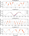 |
Fig. 1 Example light curves of Krylov from four different apparitions: 2006 (this work); 2010 (Wright et al. 2010 and Mainzer et al. 2011); 2016 (Lee et al. 2017); 2017 (this work). Solid curves represent synthetic light curves provided by the best-fit solution. The start times of each light curve are mentioned in the titles. |
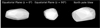 |
Fig. 2 Convex shape model of Krylov. |
4 Discussion
In this section we examine some physical effects acting on Krylov to understand its current spin state and rotational evolution. Since Krylov is an MBA and belongs to the Phocaea asteroid family with an age of about 2.2 Gyr (Carruba 2009), we considered three possible mechanisms: the YORP effect, the damping effect, and sub-catastrophic impact. According to the physical model of Krylov in Table 2, its excitation level is at about 2% excited state compared to a PA rotation state. A comparison of the excitation level with those of other known tumblers with available physical models shows that the excitation level of Krylov is similar to those of (99942) Apophis (E∕E0 ~ 1.02; Pravec et al. 2014) and (214869) 2007 PA8 (~1.08; Brozović et al. 2017), and quite lower than those of 2008 TC3 (~ 1.21; Scheirich et al. 2010), ‘Oumuamua (~1.98; Mashchenko 2019), and (4179) Toutatis (~2.08; Hudson & Ostro 1995). The small difference in the spin state of Krylov compared to its PA-rotation state can be attributed to (1) excitation of the asteroid by a low-magnitude force and (2) substantial damping of its NPA spin state from a higher excited-rotation state.
In order to find the most likely mechanism for maintaining its current spin state, we estimated timescales for Krylov. The physical parameters of Krylov used to estimate the timescales are as follows: D = 7.716 km (Mainzer et al. 2019), a = 2.33 AU (Minor Planet Center), andP1 = 82.28 h (this work). P1 is the strongest apparent period, the conjunction period between Pψ and Pϕ. The diameter is one of the parameters to calculate the timescale. However, Krylov diameters determined in previous studies are inconsistent with each other: 10.44 ± 0.37 km (AKARI; Usui et al. 2011), 7.716 ± 0.043 km (WISE1; Mainzer et al. 2019), and 8.655 ± 0.557 km (WISE2; Mainzer et al. 2019). These discrepancies are not critical, however, because the timescales are based on order of magnitude estimate. Nevertheless, to clarify its diameter, we examined observation data used in each of these studies (see Table 3). AKARI and WISE2 data were acquired using a lower number of observational passbands and fewer observation points than WISE1. Therefore, the diameter based on WISE1 data was considered the most reliable and was used for timescale estimation.
The collisional timescale (τcollision) for an MBA can be estimated as

where R is the radius of an asteroid in meters (Farinella et al. 1998).
At the same time, we considered the damping timescale (τdamping) of a tumbling asteroid. It is the timescale over which NPA rotation shifts to PA rotation due to the dissipation of stress and strain forces. This timescale is calculated as
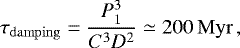
where C denotes a constant of 36, and D, P1, and τdamping are in kilometers, hours, and Gyr (Pravec et al. 2014), repectively.
In addition, we estimated the YORP timescale (τYORP) for reaching the onset of tumbling spin state driven by the YORP effect as
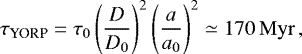
where τ0 = 5.3 Kyr was the previously determined value for D0 = 50 m, a0 = 2 AU and a reference initial rotation period P0 = 6 h as reported by Vokrouhlický et al. (2007). Should the initial rotation period be longer than P0, the estimated YORP timescale would be shorter. On the other hand, the above-mentioned result was based on a simple approach to YORP effect considering only large-scale shape modeling. Small-scale irregularities of an asteroid surface, unresolved by our model, can typically diminish the strength of the resulting YORP effect. A similar trend has also been found when comparing detected YORP values with their predictions (Vokrouhlický et al. 2015). A fudge factor of 2 to 3 in extending the estimated YORP timescale may be thus expected.
From the timescales calculated above, it is very difficult to understand why Krylov becomes an NPA spinner with an excitation level of about 2%. Nonetheless, it seems certain for Krylov that the timescale of the YORP effect is comparable to that of the damping effect. This may imply that the rotational kinetic energy loss by the strain-stress force may be simultaneously balanced by the YORP effect. Furthermore, it can be supposed that occasional collisions within the age of the Phocaea asteroid family maintain Krylov’s present NPA rotation against the PA rotation.
Physical model of Krylov.
Parameters of AKARI, WISE1, and WISE2 observations.
Acknowledgements
We are very thankful to the reviewer, Dr. M. Drahus for his positive criticisms, suggestions, and comments which greatly improved the original version of the manuscript. This research is supported by Korea Astronomy and Space Science Institute (KASI). Work at KASI was partly supported under the framework of international cooperation program managed by the National Research Foundation of Korea (2017K2A9A1A06037218, FY2018). The work of J. Ďurech and M. Lehký was supported by the grant 18-04514J of the Czech Science Foundation. The work of C.-H. Kim was financially supported by the Research Year of Chungbuk National University in 2018. The work at Modra was supported by the Slovak Grant Agency for Science VEGA, Grant 1/0911/17. M.K. and O.E. thank to TÜBİTAK for a partial support in using T100 telescope with project number 14BT100-648. This research has made use of the KMTNet system operated by the Korea Astronomy and Space Science Institute (KASI) and the data were obtained at three host sites of CTIO in Chile, SAAO in South Africa, and SSO in Australia. The Joan Oró Telescope (TJO) of the Montsec Astronomical Observatory (OAdM) is owned by the Catalan Government and operated by the Institute for Space Studies of Catalonia (IEEC). This publication also makes use of data products from NEOWISE, which is a project of the Jet Propulsion Laboratory/California Institute of Technology, funded by the Planetary Science Division of the National Aeronautics and Space Administration.
Appendix A Additional table
Observational and instrument details.
References
- Belton, M. J. S., Hainaut, O. R., Meech, K. J., et al. 2018, ApJ, 856, L21 [NASA ADS] [CrossRef] [Google Scholar]
- Bertin, E. 2010, Astrophysics Source Code Library [record ascl:1010.063] [Google Scholar]
- Bottke, W. F., Brož, M., O’Brien, D. P., et al. 2015, in Asteroids IV, eds. P. Michel, F. E. DeMeo, & W. F. Bottke (Tucson: University of Arizona Press), 701 [Google Scholar]
- Brozović, M., Benner, L. A. M., Magri, C., et al. 2017, Icarus, 286, 314 [NASA ADS] [CrossRef] [Google Scholar]
- Carruba, V. 2009, MNRAS, 398, 159 [NASA ADS] [CrossRef] [Google Scholar]
- Chambers, K. C., Magnier, E. A., Metcalfe, N., et al. 2016, arXiv e-prints, [arXiv:1612.05560] [Google Scholar]
- Cutri, R. M., Wright, E. L., Conrow, T., et al. 2012, Explanatory Supplement to the WISE All-Sky Data Release Products, Tech. rep. [Google Scholar]
- Drahus, M., Guzik, P., Waniak, W., et al. 2018, Nat. Astron., 2, 407 [NASA ADS] [CrossRef] [Google Scholar]
- Ďurech, J., Hanuš, J., & Alí-Lagoa, V. 2018, A&A, 617, A57 [NASA ADS] [CrossRef] [EDP Sciences] [Google Scholar]
- Farinella, P., Vokrouhlický, D., & Hartmann, W. K. 1998, Icarus, 132, 378 [NASA ADS] [CrossRef] [Google Scholar]
- Fraser, W. C., Pravec, P., Fitzsimmons, A., et al. 2018, Nat. Astron., 2, 383 [NASA ADS] [CrossRef] [Google Scholar]
- Gilliland, R. L., & Brown, T. M. 1988, PASP, 100, 754 [NASA ADS] [CrossRef] [Google Scholar]
- Hapke, B. 1993, Theory of Reflectance and Emittance Spectroscopy (Cambridge: Cambridge University Press) [Google Scholar]
- Harris, A. W. 1994, Icarus, 107, 209 [NASA ADS] [CrossRef] [Google Scholar]
- Howell, S. B. 1989, PASP, 101, 616 [NASA ADS] [CrossRef] [Google Scholar]
- Hudson, R. S., & Ostro, S. J. 1995, Science, 270, 84 [NASA ADS] [CrossRef] [Google Scholar]
- Kaasalainen, M. 2001, A&A, 376, 302 [NASA ADS] [CrossRef] [EDP Sciences] [Google Scholar]
- Kaasalainen, M., & Torppa, J. 2001, Icarus, 153, 24 [NASA ADS] [CrossRef] [Google Scholar]
- Kaasalainen, M., Torppa, J., & Muinonen, K. 2001, Icarus, 153, 37 [NASA ADS] [CrossRef] [Google Scholar]
- Kim, S.-L., Park, B.-G., & Chun, M.-Y. 1999, A&A, 348, 795 [NASA ADS] [Google Scholar]
- Kim, S.-L., Lee, C.-U., Park, B.-G., et al. 2016, J. Korean Astron. Soc., 49, 37 [NASA ADS] [CrossRef] [Google Scholar]
- Lee, H.-J., Moon, H.-K., Kim, M.-J., et al. 2017, J. Korean Astron. Soc., 50, 41 [NASA ADS] [CrossRef] [Google Scholar]
- Li, J. Y., Helfenstein, P., Buratti, B., Takir, D., & Clark, B. E. 2015, in Asteroids IV, eds. P. Michel, F. E. DeMeo, & W. F. Bottke (Tucson: University of Arizona Press), 129 [Google Scholar]
- Mainzer, A., Bauer, J., Grav, T., et al. 2011, ApJ, 731, 53 [NASA ADS] [CrossRef] [Google Scholar]
- Mainzer, A. K., Bauer, J. M., Cutri, R. M., et al. 2019, NASA Planetary Data System, NEOWISE Diameters and Albedos V2. 0. [Google Scholar]
- Marsden, B. G., & Williams, G. V. 1993, MPC, 22507 [Google Scholar]
- Mashchenko, S. 2019, MNRAS, 489, 3003 [NASA ADS] [CrossRef] [Google Scholar]
- Nesvorny, D. 2015, NASA Planetary Data System, EAR [Google Scholar]
- Pravec, P., Harris, A. W., Scheirich, P., et al. 2005, Icarus, 173, 108 [NASA ADS] [CrossRef] [Google Scholar]
- Pravec, P., Wolf, M., & Sarounova, L. 2006, Ondrejov Asteroid Photometry Project [Google Scholar]
- Pravec, P., Scheirich, P., Ďurech, J., et al. 2014, Icarus, 233, 48 [NASA ADS] [CrossRef] [Google Scholar]
- Prendergast, K. H. 1958, AJ, 63, 412 [NASA ADS] [CrossRef] [Google Scholar]
- Press, W. H., Flannery, B. P., & Teukolsky, S. A. 1986, Numerical Recipes. The Art of Scientific Computing (Cambridge: Cambridge University Press) [Google Scholar]
- Scheirich, P., Durech, J., Pravec, P., et al. 2010, Meteorit. Planet. Sci., 45, 1804 [NASA ADS] [CrossRef] [Google Scholar]
- Tonry, J. L., Stubbs, C. W., Lykke, K. R., et al. 2012, ApJ, 750, 99 [NASA ADS] [CrossRef] [Google Scholar]
- Usui, F., Kuroda, D., Müller, T. G., et al. 2011, PASJ, 63, 1117 [NASA ADS] [CrossRef] [Google Scholar]
- Vokrouhlický, D., Breiter, S., Nesvorný, D., & Bottke, W. F. 2007, Icarus, 191, 636 [NASA ADS] [CrossRef] [Google Scholar]
- Vokrouhlický, D., Bottke, W. F., Chesley, S. R., Scheeres, D. J., & Statler, T. S. 2015, in Asteroids IV, eds. P. Michel, F. E. DeMeo, & W. F. Bottke (Tucson: University of Arizona Press), 509 [Google Scholar]
- Walsh, K. J., & Jacobson, S. A. 2015, in Asteroids IV, eds. P. Michel, F. E. DeMeo, & W. F. Bottke (Tucson: University of Arizona Press), 375 [Google Scholar]
- Warner, B. D. 2006, A Practical Guide to Lightcurve Photometry and Analysis (Berlin: Springer) [Google Scholar]
- Warner, B. D., Harris, A. W., & Pravec, P. 2009, Icarus, 202, 134 [NASA ADS] [CrossRef] [Google Scholar]
- Wright, E. L., Eisenhardt, P. R. M., Mainzer, A. K., et al. 2010, AJ, 140, 1868 [NASA ADS] [CrossRef] [Google Scholar]
All Tables
All Figures
|
Fig. 1 Example light curves of Krylov from four different apparitions: 2006 (this work); 2010 (Wright et al. 2010 and Mainzer et al. 2011); 2016 (Lee et al. 2017); 2017 (this work). Solid curves represent synthetic light curves provided by the best-fit solution. The start times of each light curve are mentioned in the titles. |
| In the text | |
|
Fig. 2 Convex shape model of Krylov. |
| In the text | |
Current usage metrics show cumulative count of Article Views (full-text article views including HTML views, PDF and ePub downloads, according to the available data) and Abstracts Views on Vision4Press platform.
Data correspond to usage on the plateform after 2015. The current usage metrics is available 48-96 hours after online publication and is updated daily on week days.
Initial download of the metrics may take a while.