| Issue |
A&A
Volume 635, March 2020
|
|
|---|---|---|
| Article Number | A191 | |
| Number of page(s) | 13 | |
| Section | Planets and planetary systems | |
| DOI | https://doi.org/10.1051/0004-6361/201936692 | |
| Published online | 01 April 2020 | |
Spatial distribution of exoplanet candidates based on Kepler and Gaia data
Astronomical Institute, Slovak Academy of Sciences,
05960
Tatranská Lomnica,
Slovak Republic
e-mail: amaliuk@ta3.sk, budaj@ta3.sk
Received:
13
September
2019
Accepted:
5
February
2020
Context. Surveying the spatial distribution of exoplanets in the Galaxy is important for improving our understanding of planet formation and evolution.
Aims. We aim to determine the spatial gradients of exoplanet occurrence in the Solar neighbourhood and in the vicinity of open clusters.
Methods. We combined Kepler and Gaia DR2 data for this purpose, splitting the volume sampled by the Kepler mission into certain spatial bins. We determined an uncorrected and bias-corrected exoplanet frequency and metallicity for each bin.
Results. There is a clear drop in the uncorrected exoplanet frequency with distance for F-type stars (mainly for smaller planets), a decline with increasing distance along the Galactic longitude l = 90°, and a drop with height above the Galactic plane. We find that the metallicity behaviour cannot be the reason for the drop of the exoplanet frequency around F stars with increasing distance. This might have only contributed to the drop in uncorrected exoplanet frequency with the height above the Galactic plane. We argue that the above-mentioned gradients of uncorrected exoplanet frequency are a manifestation of a single bias of undetected smaller planets around fainter stars. When we correct for observational biases, most of these gradients in exoplanet frequency become statistically insignificant. Only a slight decline of the planet occurrence with distance for F stars remains significant at the 3σ level. Apart from that, the spatial distribution of exoplanets in the Kepler field of view is compatible with a homogeneous one. At the same time, we do not find a significant change in the exoplanet frequency with increasing distance from open clusters. In terms of byproducts, we identified six exoplanet host star candidates that are members of open clusters. Four of them are in the NGC 6811 (KIC 9655005, KIC 9533489, Kepler-66, Kepler-67) and two belong to NGC 6866 (KIC 8396288, KIC 8331612). Two out of the six had already been known to be cluster members.
Key words: planetary systems / stars: formation / stars: rotation / stars: statistics / solar neighborhood
© ESO 2020
1 Introduction and motivation
The stellar environment within our Galaxy is far from homogeneous and isotropic. The Galaxy has a spiral structure and the disc undergoes large-scale perturbations caused by the spiral arms. Another important source of inhomogeneity is in the form of shock waves generated by supernova explosions. These events enrich the interstellar medium with heavy elements and work as a trigger for star and planet formation. Even within the disk, there are stars of different ages, populations, and metallicities. For field stars, the age-metallicity relation is nearly flat up to 8 Gyr with a clear drop in the metallicity for older stars. Metallicity decreases with the Galactocentric radius and height above the Galactic plane (Bergemann et al. 2014; Duong et al. 2018). The nitrogen and oxygen abundances of Galactic HII regions were also found to decrease with the Galactocentric radius (Esteban et al. 2017; Esteban & García-Rojas 2018). Open clusters constitute “islands” of stars with homogeneous ages and metallicity. They differ from neighbourhood field stars by the enhanced spatial density of their stars. The metallicity of open clusters decreases with the distance from the Galaxy centre and increases with the age of the cluster (Netopil et al. 2016; Jacobson et al. 2016). Such inherent inhomogeneity of the environment may have an impact on planet formation and occurrence. For example, the frequency of the exoplanets occurrence depends on metallicity. Short-period gas giants (hot Jupiters and warm sub-Neptunes) are more likely to be found around metal-rich stars while smaller planets are found around stars with a wide range of metallicities (Fischer & Valenti 2005; Buchhave et al. 2012; Narang et al. 2018; Petigura et al. 2018). Planets may migrate over the course of their formation and their evolution, which impacts the chances of their detection significantly. Hot Jupiters were most probably born beyond the snow line and migrated inward, affecting all the inner planets.
Unfortunately, we know very little about young exoplanets. van Eyken et al. (2012) found a transiting exoplanet candidate orbiting a T Tau star in the Orion-OB1a/25-Ori region. Meibom et al. (2013) discovered two mini-Neptunes (Kepler-66, Kepler-67) in the 1 Gyr cluster NGC 6811 which is in the Kepler field of view. They concluded that the frequency of planets in this cluster is approximately equal to the field one. Curtis et al. (2018) identified a sub-Neptune exoplanet transiting a solar twin EPIC 219800881(K2-231) in the Ruprecht 147 stellar cluster. This indicates an exoplanet frequency of the same order of magnitude as in NGC 6811. Quinn et al. (2012) detected two hot Jupiters in the Praesepe cluster and estimated a lower limit of 3.8 + 5.0 − 2.4% on the hot Jupiter frequency in this metal-rich open cluster. Given the known age of the cluster, this also demonstrates that giant planet migration occurred within 600 Myr after the formation. Libralato et al. (2016) presents the sample of seven exoplanet candidates discovered in the Praesepe field. Two of them, K2-95 and EPIC 211913977, are members of the cluster. Mann et al. (2017) found seven transiting planet candidates in Praesepe cluster from the K2 light curves (K2-100b, K2-101b, K2-102b, K2-103b, K2-104b, EPIC 211901114b, K2-95b). Six of them were confirmed to be real planets, with the last one requiring more data. K2-95b was also studied in Pepper et al. (2017). Rizzuto et al. (2017) studied nine known transiting exoplanets in the clusters (Hyades, Upper Scorpius, Praesepe, Pleiades) and also identified one new transiting planet candidate orbiting a potential Pleiades member. The lack of detected multiple systems in the young clusters is consistent with the expected frequency from the original Kepler sample within our detection limits. Rizzuto et al. (2019) addressed the question of planet occurrence in the young clusters observed by the K2 mission. Initial results indicate that planets around 650–750 Myr M-dwarfs have inflated radii but a similar frequency of occurrence compared to their older counterparts. However, the 125 Myr old Pleiades has a lower occurrence rate of short period planets. In Praesepe, Rizzuto et al. (2018) also discovered atwo-planet system of K2-264. Both planets are likely mini-Neptunes. K2-264 is one of two multiple-planet systems found in the open clusters. The other is K2-136, a triple transiting-planet system in the Hyades cluster (Mann et al. 2018; Livingston et al. 2018). K2-136 system includes an Earth-sized planet, a mini-Neptune, and a super-Earth orbiting a K-dwarf. Gaidos et al. (2017) describes a “super-Earth-size” planet transiting an early K dwarf star observed by the K2 mission. The host star, EPIC 210363145, was identified as a member of the Pleiades cluster, but a more detailed analysis of the star’s properties did not confirm its cluster membership. Vanderburg et al. (2018) reported the discovery of a long-period transiting exoplanet candidate with the mass of about 6.5 M⊕, called HD 283869b, orbiting another K-dwarf in the Hyades cluster.
The Young Exoplanet Transit Initiative (YETI) project conducts searches for transiting exoplanets in a number of young open clusters. The detection rate is lower than expected, which may be due to an intrinsic stellar variability or the true paucity of such exoplanets (Neuhäuser et al. 2011; Errmann et al. 2014; Garai et al. 2016; Fritzewski et al. 2016). The theoretical study of Bonnell et al. (2001) indicates that while planetary formation is heavily suppressed in the crowded environment of the globular clusters, less crowded systems such as open clusters should have a reduced effect on any planetary system. Fujii & Hori (2019) also explored the survival rates of planets against stellar encounters in open clusters by performing a series of N-body simulations of high-density and low-density open clusters, along with open clusters that grow via mergers of sub-clusters, and embedded clusters. They found that less than 1.5% of close-in planets within 1 AU and at most 7% of planets within 1–10 AU from the star are ejected by stellar encounters in clustered environments. The ejection rate of planets at 10–100 AU around FGKM-type stars reaches a few tens of percent.
Another piece of evidence to demonstrate that planet formation is affected by the presence of a more distant stellar companion comes from the study of binary stars. Wang et al. (2014a,b) found that the circumstellar planet occurrence in such systems is significantly lower than in single stars, indicating that the planet formation is significantly suppressed in this case. In the end, the question of the spatial distribution of exoplanets and their host stars or, more precisely, the local frequency of their occurrence throughout the Galaxy presents an unsolved problem intimately linked to the planet’s formation and evolution.
The Kepler mission provides the most complete and homogeneous sample of exoplanets and their host stars to date (Borucki et al. 2010). On the other hand, the recent second data release of Gaia (Gaia Collaboration 2016, 2018) provides the most precise distances to the stars. Together, the Kepler and Gaia data provide the best information about the spatial distribution of exoplanets available at present. The goal of this study is not to provide an absolute estimate of exoplanet occurrence; rather, we aim to search for relative variations in the planet occurrence in the space on (a) longer scales spanning hundreds to thousands of parsecs or (b) shorter scales of tens of parsecs in the vicinity of open clusters. As a by product of this analysis, we identify exoplanet candidates which are members of the open clusters in the Kepler field of view.
2 Stellar sample
We start with the list of the Kepler target stars (KSPC DR 25) from Mathur et al. (2017), which counts about 190 000 stars. The positions of all these stars were cross-matched with the Gaia DR2 positions in Berger et al. (2018). They used the X-match service of the Centre de Données astronomiques de Strasbourg (CDS) and applied the following criteria to match the stars: the difference in the position smaller than 1.5 arcseconds; and the difference in the magnitudes smaller than two magnitudes. For stars with multiple matches that satisfied these criteria, the authors decided to keep those with the smallest angular separations. Apart from that, the following stars were removed from the sample: stars with poorly determined parallaxes (σπ ∕π > 0.2), stars with low effective temperatures (Teff < 3000 K), stars with either extremely low gravity (logg < 0.1) (in CGS units), or a low-quality Two Micron All-Sky Survey (Cutri et al. 2003) photometry (lower than “AAA”). Following this procedure, the sample contained 177, 911 Kepler target stars and 3084 Kepler host star candidates with 4044 exoplanet candidates.
In the next step, we excluded giant stars from the sample. We put the following limitations on stellar radius from Fulton et al. (2017): Rstar ∕R⊙ < 100.00025(Teff−5500)+0.20. Using this criterion, we rejected 57 743 giants of all types. The final list contains 120 168 Kepler target stars, including 2562 Kepler host star candidates with 3441 exoplanet candidates. Kepler target stars may have different spectral types. Most of them are F, G, and K star. These stars each have a different brightness and are seen up to different distances, which might cause biases in our analysis. That is why we further broke the stellar sample up into three categories: F stars with 6000 K ≤ Teff ≤ 7500 K, G stars with 5200 K ≤ Teff ≤ 6000 K, and K stars with 3700 K ≤ Teff ≤ 5200 K. There are 35075 K-stars, 64 525 G-stars, 17 750 F-stars, and 2818 other types of stars in the final sample.
Apart from the star and planet sample, we used other stellar properties such as the metallicities in the form of [Fe/H] from the Kepler stellar properties catalogue KSPC DR 25 and coordinates, effective temperatures, parallaxes, and G-band magnitudes from Gaia DR2 (Gaia Collaboration 2016, 2018). We note that Gaia DR2 parallaxes are affected by a zero-point offset (Arenou et al. 2018; Riess et al. 2018; Zinn et al. 2019; Khan et al. 2019). This offset was taken into accountby adding + 0.029 mas (global value of zero-point) to all parallaxes before they were converted to distances (Lindegren et al. 2018).
3 Spatial gradients of the exoplanet frequency
3.1 Uncorrected exoplanet frequency behaviour
To study the spatial distribution of exoplanets, we divided the space into a number of smaller 3D segments according to the right ascension α, declination δ, and distance from the Sun r. The Kepler field of view (see Fig. 1) is composed of 21 fields (associated with individual chips) with small gaps in between. That is why we created 21 spatial beams corresponding to these fields. Consequently, we split each beam into five segments according to the distance. In this way, we obtained 21 × 5 = 105 spatial bins. In each bin, we calculated the ratio of the number of exoplanet candidates and Kepler target stars which we will call the uncorrected exoplanet frequency. We would like to point out that this frequency is not corrected for observing and completeness biases (see Sect. 3.2) and, thus, it is not a real exoplanet frequency, but a relative quantity proportionalto it. We only use it as a guide to search for patterns that are worthy of more attention. Then we assigned (r, α, δ) coordinates to each bin such that they were simply the centre of the bin. We explored the gradients in different coordinate systems that is why we assigned to the center of each bin also the (rg, z) coordinates of the Galactocentric system and (x, y, z) coordinates of the Cartesian system, where rg is the projection of Galactocentric radius on the galactic plane and z is the distance from the galactic plane. The x-axis of the Cartesian coordinate system is directed towards the centre of the Galaxy, y-axis is along the Galactic longitude 90° and z-axis is the same as above. Then we approximated the uncorrected exoplanet frequency with the following linear functions:
 (1)
(1)
 (2)
(2)
 (3)
(3)
When fitting Eqs. (1)–(3), we assumed a Gaussian likelihood and used standard linear model fitting techniques for reporting uncertainties in the parameters. We adopted bins with no counts of a zero value during the fit. Since we used the results of this fit as an indicator of which relationships to explore with a higher fidelity model, in Sect. 3.2, we do not explore whether a more sophisticated model fitting (e.g. Poisson likelihood, upper limits, etc.) would significantly alter the fit model parameters. Because F, G, and K stars have different brightness and are seen up to different distances, we analysed them separately. To create a volume-limited sample, we assumed some initial threshold visual G-band magnitude of 16 mag and calculated the distances corresponding to typical F, G, and K main sequence stars. The location of stars of different spectral class satisfying this criterion is displayed in Fig. 2 in a Cartesian system aligned with the galactic coordinates.
The 16-magnitude threshold would correspond to a maximum distance of 250, 1000, and 2190 pc for K, G, and F stars, respectively.Then we split this maximum distance into five equal bins as mentioned above. Apart from the brightness of the star, the planet detection efficiency depends on the transit depth and, hence, on the planet radius. Planet occurrence itself may depend on the planet size. That is why we also split the sample of exoplanets candidates into the following intervals according to their radius: Rplanet ≥ 0.75 R⊕, which covers most of the planets; 0.75 R⊕ < Rplanet ≤ 1.75 R⊕, which covers Earth-like planets and super-Earths; 1.75 R⊕ < Rplanet ≤ 3.0 R⊕, which covers sub-Neptunes; and Rplanet > 3.0 R⊕, which corresponds mostly to hot Jupiters. Then we fit for (kr, kα, kδ, k0), (krg, kz, k0), and (kx, ky, kz, k0) coefficients. Apart from k0, they correspond to the spatial gradients of the uncorrected exoplanet frequency in different coordinate systems. The results are listed in Tables A.1–A.3.
As can be seen in the tables, the exoplanet frequency gradients along the α and δ coordinates are not statistically significant. They are compatible with zero (within 2σ errors)1. Nevertheless, we find a statistically significant negative kr value of the gradient in the distance r for all the planets around F stars except those with Rplanet ≥ 3.0 R⊕. We do not find any significant gradient of the exoplanet frequency with the Galactocentric radius. However, again, for all the planets around the F stars (except those with Rplanet ≥ 3.0 R⊕) we find statistically significant negative values of kz, the gradient in the height above the Galactic plane. At the same time, we find significant negative gradients along the y axis for the same stars (F stars). Since we are observing the significant trends based on the uncorrected planet counts, we explore in Sect. 3.2 whether these trends are intrinsic to the Galaxy or whether the trends have been injected by detection biases.
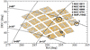 |
Fig. 1 Location of exoplanet host stars (orange dots), Kepler target stars (grey dots), and open clusters (asterisks) in the Kepler field of view. Circles around some open clusters indicate the size of the inner cylinders used for statistics; see Sect. 5 for more details. |
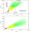 |
Fig. 2 Location of the Kepler target stars in the Galactic disc in (x, y) plane (upper panel) and (y, z) plane (lower panel). F, G, and K stars are highlighted with green, yellow, and red dots, respectively. The X-axis points to the Galactic centre. The direction of the Y-axis corresponds to the Galactic longitude of 90°. The three curves of constant Galactocentric radius are also plotted. |
3.2 Discussion, bias correction, interpretation, and disentangling
The transit method of exoplanet detection suffers from heavy biases. Its efficiency depends on the planet-to-star radius ratio, orbital period, eccentricity, inclination, and stellar brightness. Such biases in the Kepler data were included in recent studies by Mulders et al. (2018), van Sluijs & Van Eylen (2018), Zhu et al. (2018), Petigura et al. (2018) or Kipping & Sandford (2016). Given that our sample is homogeneous. Most of these biases will be the same over the whole field of view, except for the distance bias. Distance bias reduces the number of small planets detected with the distance from the observer since it is more difficult to find small planets around fainter stars. We notice that F stars are the ones that sample the largest distances. It is also notable that the kr values gradually drop and become more significant with decreasing the planet radius, indicating that this trend may be due to an above-mentioned observational distance bias.
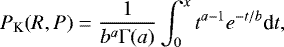
Apart from the above remarks, we note a strong correlation between the distance r and the y-coordinate, as well as a correlation between the y and z-coordinate for the stars in the Kepler field of view (see Fig. 2). Consequently, any gradient along the distance might reflect mainly onto a gradient along the y coordinate of the Cartesian system or along the z coordinate of the Galactocentric system. This is precisely what we found and that is why we need to correct for such a bias. We followed Burke et al. (2015), who suggested a method of deriving an exoplanet occurrence which takes into account all aforementioned biases. Due to its numerical efficiency, we adopted the Burke et al. (2015) model for the Kepler pipeline completeness rather than the more accurate and recent model from Burke & Catanzarite (2017). The Burke et al. (2015) model describes the algorithm for calculation of probability that the transit event will be detected:
 (4)
(4)
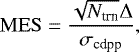
where PK is the signal recoverability of the Kepler pipeline for planet with given radius R and orbital period P. The best-fit coefficients to the sensitivity curve are a = 4.35, b = 1.05 as found by Christiansen et al. (2015). The integral boundary x = MES − 4.1 − (MESthresh − 7.1). MES (Multiple Event Statistics) depends on the transit depth, observation errors and the number of observed transits:
 (5)
(5)
where Ntrn = (Tobs∕P) × fduty is the expected number of transits, Tobs is the time baseline of observational coverage for a target and fduty is the observing duty cycle. The fduty is defined as the fraction of Tobs with valid observations. Δ is the expected transit signal depth. The robust root-mean-square (RMS) combined differential photometric precision (CDPP) σcdpp is an empirical estimate of the noise in the relative flux time series observations. The MES_thres reflects the transit-signal significance level achieved by the transiting planet search (TPS) module. The probability that a transit of a planet will be detected during the time of observation is
 (6)
(6)
where Pwin is the window function probability of detecting at least three transits. It can be explicitly written out in the binomial approximation as
 (7)
(7)
where M = Tobs∕Porb. Using these equations and parametric model for the planet distribution function (PLDF) presented by Youdin (2011) we can estimate the expected number of detectable exoplanets in each spatial bin, Nexp:
![\begin{equation*} N_{\textrm{exp}}=F_{\textrm{0}}C_{\textrm{n}}\int_{P_{\textrm{min}}}^{P_{\textrm{max}}}\int_{R_{\textrm{min}}}^{R_{\textrm{max}}} \left[\sum\limits_{j=1}^N\eta_j(R,P)\right]\times g(R,P)\textrm{d}P\textrm{d}R,\end{equation*}](/articles/aa/full_html/2020/03/aa36692-19/aa36692-19-eq8.png) (8)
(8)
where, g(R, P) describes the exoplanet distribution by radii and orbital periods:
![\begin{align*} &g(R,P)=\nonumber\\ &\begin{cases} \left(\frac{P}{P_0}\right)^{\beta_1}\left(\frac{R}{R_0}\right)^{\alpha_1}\!,\: {\rm{if}}\: {R}<{R}_{\textrm{brk}}\: {\rm{and}}\: {P}<{P}_{\textrm{brk}} \\[3pt] \left(\frac{P}{P_0}\right)^{\beta_2} \left(\frac{P_{\textrm{brk}}}{P_0}\right)^{\beta_1-\beta_2} \left(\frac {R}{R_0}\right)^{\alpha_1}\!, \: {\rm{if}}\: {R}<{R}_{\textrm{brk}}\: {\rm{and}}\: {P}\ge {P}_{\textrm{brk}} \\[3pt] \left(\frac{P}{P_0}\right)^{\beta_1}\left(\frac {R}{R_0}\right)^{\alpha_2} \left(\frac{R_{\textrm{brk}}}{R_0}\right)^{\alpha_1-\alpha_2}\!,\: {\rm{if}}\: {R}\ge {R}_{\textrm{brk}}\: \textrm{{and}}\: {P}<{P}_{\textrm{brk}} \\[3pt] \left(\frac{P}{P_0}\right)^{\beta_2} \left(\frac{P_{\textrm{brk}}}{P_0}\right)^{\beta_1-\beta_2} \left(\frac {R}{R_0}\right)^{\alpha_2}\left(\frac{R_{\textrm{brk}}}{R_0}\right)^{\alpha_1-\alpha_2} \: {\rm{if}}\: {R}\ge {R}_{\textrm{brk}}\: \textrm{{and}}\: {P}\ge {P}_{\textrm{brk}}. \end{cases}\end{align*}](/articles/aa/full_html/2020/03/aa36692-19/aa36692-19-eq9.png) (9)
(9)
This PLDF model is modified by the per-star transit survey effectiveness (or perstar pipeline completeness), ηj, summed over N targets in the sample. It can be expressedas ηj = Pdet,j × Ptr,j where Ptr,j= (R⋆∕a)(1 − e2) is the geometric probability of a planet to transit the star. The Cn is determined from the normalisation requirement,
 (10)
(10)
F0 is an average number of planets per star in the sample, or real exoplanet occurrence. We calculate it via a maximisation of the Poisson likelihood, L, of the data from a survey that detects Npl planets (in our case, it is the number of detected exoplanets in each bin) around N survey targets:
![\begin{equation*} L \sim \left[ F_0^{N_{\textrm{pl}}}C_n^{N_{\textrm{pl}}}\prod\limits_{i = 1}^{N_{\textrm{{pl}}}}g(R_i,P_i) \right]\textrm{exp}\left(-N_{\textrm{exp}}\right).\end{equation*}](/articles/aa/full_html/2020/03/aa36692-19/aa36692-19-eq11.png) (11)
(11)
As it follows from maximisation condition, in the case of the fixed parameters for Rbrk, Pbrk, α1, α2, β1, β2, the value of exoplanet occurrence for each bin may be obtained as a point where derivative of L is equal to zero:
 (12)
(12)
Upon solving this equation, we get an exoplanet occurrence:
![\begin{equation*} F_0=\frac{N_{\textrm{pl}}}{C_{\textrm{n}}\int_{P_{\textrm{min}}}^{P_{\textrm{max}}}\int_{R_{\textrm{min}}}^{R_{\textrm{max}}} \left[\sum\limits_{j=1}^N\eta_j(R,P)\right]\times g(R,P)\textrm{d}P\textrm{d}R}.\end{equation*}](/articles/aa/full_html/2020/03/aa36692-19/aa36692-19-eq13.png) (13)
(13)
Rather than simultaneously determine all parameters in the model, we reduce the dimensionality of the problem and impose a prior on the model by assuming that the PLDF parameters are fixed at values determined in the literature. This allows us to study the real planet occurrence in more detail, rather than focusing on a global fit allowing for all parameters to vary. We use the following values of free parameters: Rbrk= 0.94, α1 = 19.68, α2 = −1.78, β2 = −0.65 from Burke et al. (2015). Unfortunately, the authors only analysed a region from 50 < P < 300 days and 0.75 < R < 2.5 REarth, so we adopted Pbrk = 7.0 and β1 = 2.23 from Youdin (2011). In this work, the authors use the same sample of exoplanets and their values of parameters are in good agreement with those ones from Burke et al. (2015) for P > 50 days. We limit our integrals for determining Nexp with Pmin = 0 d, Pmax = 300 d. We adopt ranges of our subsamples described in previous section as limits for R. We chose 0.5 days as the bin size for period and 0.02 REarth as the bin size for planet radii to be sure that we have enough bins for reliable calculation of integrals. During the computation of gradients, we ignore bins where the number of expected planets Nexp is less than one and, simultaneously, the number of detected planets is zero. The new gradients corresponding to these corrected exoplanet occurrences in different coordinate systems, F0(r, α, δ), F0(rg, z), F0(x, y, z), are listed in the Tables 1–3. The real exoplanet frequency is much larger than the uncorrected frequency of occurrence and the same is true for its gradient error. As a result, the gradients are significantly larger than in the previous case. However, most of the gradients which were previously found to be significant became statistically insignificant after the bias correction. Only the negative gradient along the distance in spherical coordinates, kr, is still significant at the 3σ level. It remains to be verified by future observations if this behaviour is real. Apart from that, the exoplanet frequency of occurrence obtained with this method is compatible with a homogeneous space distribution.
Gradients of corrected exoplanet frequency for stars up to 16th magnitude in spherical equatorial coordinates (r, α, δ).
Gradients of corrected exoplanet frequency for stars up to 16th magnitude in cylindrical coordinates (rg, z).
Gradients of corrected exoplanet frequency for stars up to 16th magnitude in Cartesian coordinates (x, y, z).
4 Spatial gradients of the metallicity
The above-mentioned drop in the uncorrected exoplanet frequency with the height above the Galactic plane might be related to the decrease of metallicity with the Galactocentric radius and height above the galactic plane (Bergemann et al. 2014; Duong et al. 2018; Esteban et al. 2017; Esteban & García-Rojas 2018). To check whether the above-mentioned kr, kz, ky gradients may be related to the metallicity behaviour, we also calculated the gradients of metallicity in the Kepler field exploiting the [Fe/H] values of all Kepler target stars. We calculated average metallicity in each of 105 spatial bins applying the same restrictions for the spectral types and volume as for the 16 mag limited sample before. Metallicity was approximated by the similar linear functions:
=k_r r+k_{\alpha} \alpha+k_{\delta} \delta+k_0.\end{equation*}](/articles/aa/full_html/2020/03/aa36692-19/aa36692-19-eq14.png) (14)
(14)
=k_{rg} r_g+ k_z z+ k_0. \end{equation*}](/articles/aa/full_html/2020/03/aa36692-19/aa36692-19-eq15.png) (15)
(15)
=k_{x} x+ k_y y+k_z z+ k_0. \end{equation*}](/articles/aa/full_html/2020/03/aa36692-19/aa36692-19-eq16.png) (16)
(16)
Coefficients of the fit are listed in the Tables B.1–B.3.
In the equatorial coordinates (r, α, δ), the gradients along the right ascension or declination are not statistically significant. The gradients in the distance are significant at the 2σ level but they are so low that they represent changes in [Fe/H] at the 0.01 dex level which can hardly have any effect on the planet formation and may be just an artifact of the method used.
Gradients in the Galactic (rg, z) and Cartesian (x, y, z) coordinates are more interesting. For G stars we observe a significant (>3σ) increase of metallicity with the Galactocentric radius. This gradient represents only about 0.06 dex increase of metallicity across our volume. It is not in agreement with the above-mentioned previous studies, which report the opposite tendency. For F stars in Cartesian coordinates, we observe statistically significant positive gradient ky and negative gradient kz (which is consistent with previous studies). It is worth noting that the range of z values is comparable with the thickness of the Galactic disc, while the range of y values covers only a minor part of Galaxy. Thus, the negative gradient of metallicity might have slightly contributed to the decrease of the uncorrected exoplanet occurrence with the z coordinate. Nevertheless, there are no statistically significant metallicity gradients which could explain observed trends in uncorrected exoplanet occurrence with distance and y coordinate. It is also useful to note that the metallicities from the Kepler catalog were found rather inaccurate at this level (Petigura et al. 2017).
5 Relative exoplanet frequency and metallicity in the vicinity of open clusters
There are four open stellar clusters which belong to the Kepler field of view, listed in the catalogues of Dias et al. (2002) and Cantat-Gaudin et al. (2018): NGC 6811, NGC 6819, NGC 6866, and NGC 6791 (Fig. 1). Apart from these, there is also one cluster, Skiff J1942+38.6, located on the very edge of the Kepler field. The main characteristics of these clusters are presented in Table C.1. Here the age and [Fe/H] are taken from Dias et al. (2002) and coordinates, distance, and radii are from Gaia DR2 (Cantat-Gaudin et al. 2018). Most of them are about a billion years old. Unfortunately, the location of Skiff J1942 is just beyond the edge of the Kepler field. That is why it was excluded from this study.
To check if the presence of a cluster influences the exoplanet occurrence, we estimated the exoplanet frequency at different distances from the cluster spatial centre. We note that the radii of the clusters (see Table C.1) are significantly smaller than the typical 1σ precision of the Gaia DR2 at the distance of the cluster. That is why we decided to define a cylinder-like volume around each cluster. The half-length of the cylinder, l1, is equal to 2σ precision of the Gaia distance measurements. The radius of the cylinder, r1, is arbitrarily set to 20 pc. Smaller radii would limit the volume heavily and one would not find many planets for the statistics. Larger radii would cause the angular radius of the cylinder to be larger than the field of individual Kepler chips. Then we calculate the planet frequency within this cylinder and compare it with the planet frequency in an outer shell of the cylinder. The outer shell will have the shape of a hollow cylinder which is two times bigger extending from r1 to r2 = 2 × r1 and from l1 to l2 = 2 × l1. The results are summarised in Table 4.
There are too few planets in the vicinity of NGC 6819 to draw any conclusions. The exoplanet frequency in the inner and outer cylinders around NGC 6811 and NGC 6866 indicate no variation within current error bars, which is in agreement with the observations(Meibom et al. 2013; Curtis et al. 2018) and theoretical predictions (Bonnell et al. 2001; Fujii & Hori 2019). We assumed that enhanced crowding in the clusters did not impact the planet detection efficiency since we calculated the occurrence rate per Kepler target star and not the absolute occurrence rate. However, it can be expected that enhanced crowding in clusters may increase the probability of false positives (background eclipsing binaries) since the number of “blending” stars increases.
As a byproduct of this analysis, we also studied the behaviour of the metallicity in the vicinity of these clusters. We do not find any significant difference in the metallicity in the inner and outer cylinders of NGC 6811 and NGC 6866. However, we find a slightly lower metallicity in the inner shell of NGC 6819 (−0.505) compared to its outer shell (−0.273).
Exoplanet frequency and metallicity in the vicinity of open clusters.
6 Exoplanet candidates in the open clusters
6.1 Location and proper motion criteria
As a byproduct of our analysis of exoplanet occurrence in the vicinity of open clusters, we also searched for new exoplanet candidates that are members of these open clusters. Several groups searched for exoplanets in the clusters located in the Kepler field. Mochejska et al. (2005) searched for exoplanets in NGC 6791 (19h 20m 53,0s; +37°46′18″) but did not find any. In the Kepler data, Meibom et al. (2013) discovered two mini-Neptunes (Kepler-66b and Kepler-67b or KIC 9836149b & KIC 9532052b, respectively) orbiting Sun-like stars in the cluster NGC 6811. The authors argue that such small planets can form and survive in a dense cluster environment and that it implies that the frequency and properties of planets in open clusters are consistent with those of planets around field stars in the Galaxy.
To establish whether a Kepler host star belongs to an open cluster we applied several criteria. First, we applied a proper motion criterion that assumes that proper motions of cluster members are distributed normally. We calculate for each Kepler host star its proper motion membership probability Pμ as
![\begin{equation*} P_{\mu}= \textrm{exp}\left[-\frac{(\mu_{\alpha,\textrm{cl}}-\mu_{\alpha,\textrm{st}})^2} {2(\sigma_{\alpha,\textrm{cl}}^2+\sigma_{\alpha,\textrm{st}}^2)}\right] \textrm{exp}\left[-\frac{(\mu_{\delta,\textrm{cl}}-\mu_{\delta,\textrm{st}})^2} {2(\sigma_{\delta,\textrm{cl}}^2+\sigma_{\delta,\textrm{st}}^2)}\right],\end{equation*}](/articles/aa/full_html/2020/03/aa36692-19/aa36692-19-eq17.png) (17)
(17)
where μα,cl, μδ,cl, are the proper motions of the cluster in right ascension and declination; σα,cl, σδ,cl are the dispersions of the proper motion distribution in right ascension and declination taken from Cantat-Gaudin et al. (2018); μα,st, μδ,st are the proper motions of individual stars; and σα,st, σδ,st are the errors in proper motion of individual stars, respectively.
Our second criterion is the tangential angular distance from the cluster centre. Following Kraus & Hillenbrand (2007), we use an exponential function to describe this membership probability Pρ which depends on equatorial coordinates of potential members as
 (18)
(18)
where ρ is the angular distance from the star to the centre of the cluster, and ρcl is a parameter which characterises the angular size of cluster. The angular distance is calculated in the following way:
 (19)
(19)
where  are coordinates of the cluster centre and
  are coordinates of an individual star. To obtain the parameter ρcl we took a list of cluster members from Cantat-Gaudin et al. (2018), built their distribution according to the tangential angular distance and fitted for this parameter. The resulting values of ρcl for each cluster are listed in the Table C.1.
Our third criterion is distance. There is no reason to suspect that the distribution of radial distances of cluster members is different from the tangential distances. However, the error in radial distance to the stars in Gaia DR2 is much larger than the error in the tangential distance due to small uncertainties in α and δ. For NGC 6811, which is located at the distance of 1112 pc, the error in the radial distance is about 30 pc. It is several times larger than the radius of the cluster. That is why we assume that the distribution in radial distances is normal and govern fully by the errors of the distance measurements. Hence, we define its probability Pr as
![\begin{equation*} P_{\textrm{r}}=\textrm{exp}\left[-\frac{(r_{\textrm{cl}}-r_{\textrm{st}})^2}{2(\sigma_{\textrm{r,cl}}^2+\sigma_{\textrm{r,st}}^2)}\right],\end{equation*}](/articles/aa/full_html/2020/03/aa36692-19/aa36692-19-eq22.png) (20)
(20)
where rcl is the mean distance from the Sun to the cluster, σr,cl is its dispersion (all listed in Table C.1), rst is the distance to an individual star, and σr,st is its error.
It would also be possible to use another criterion based on radial velocities. Unfortunately, Gaia DR2 does not contain radial velocities of our exoplanet host stars which are members of clusters because they are too faint.
Finally, we calculate a total probability Ptot of membership for individual stars as a product of the three above-mentioned probabilities:
 (21)
(21)
Using this equation, we checked all Kepler exoplanet host stars for their membership in the above-mentioned four open clusters. A few top-ranked stars with the highest Ptot values are listed in Table C.3. Consequently, we selected four exoplanet host star candidates that are the most probable cluster members of NGC 6811 (Kepler-66, Kepler-67, KIC 9655005, KIC 9533489) and one less promising member of this cluster (KIC 9776794). The first two of these have already been mentioned in Meibom et al. (2013). Our two members have even higher cluster probabilities, but they also have very high false positive probabilities, indicating that they may not be exoplanets. In NGC 6866, we found two highly probable members which are also exoplanet host star candidates (KIC 8331612, KIC 8396288). We found no good candidates in other clusters.
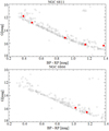 |
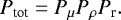
Fig. 3 Colour-magnitude diagram of clusters NGC 6811 (upper panel) and NGC 6866 (lower panel). Exoplanet host stars are marked with red circles. |
6.2 Colour-magnitude and colour-period diagrams
To verify the cluster membership of these top seven exoplanet candidates, we place them in a colour-magnitude diagram (Fig. 3) together with other cluster members taken from Cantat-Gaudin et al. (2018). All of them fit among the other members very well. Only KIC 9776794, which is the least likely member out of seven, lies slightly above the main sequence. We do not use this diagram as a separate criterion (only as a verification) since this information was already taken into account in the above-mentioned radial distance criterion. The cluster membership can be verified also by the rotational periods of the stars. Previous studies have shown that cluster members form a relatively narrow and well-defined sequence in the colour-period diagram (CPD). For example, FGK dwarfs in the Hyades (Radick et al. 1987; Delorme et al. 2011; Douglas et al. 2016), Praesepe (Delorme et al. 2011; Kovács et al. 2014), Coma Berenices (Collier Cameron et al. 2009), Pleiades (Stauffer et al. 2016), and M 37 (Hartman et al. 2009). Barnes et al. (2015) constructed a CPD for M 48 and derived its rotational age using gyro-chronology. This sequence in the CPD is followed closely by a theoretical isochrone and looks similar to the CPD of other open clusters of the same age. Barnes et al. (2016) found that rotation periods of M 67 members delineate a sequence in the CPD reminiscent of that discovered first in the Hyades cluster. Similar sequence we can see in the mass-period diagram (which is equivalent to CPD) of NGC 752 (Agüeros et al. 2018). In general, the rotational evolution theory is described in Barnes (2010), van Saders et al. (2019). Kovács et al. (2014) also found that exoplanet host stars may have shorter periods than predicted due to the tidal interaction and angular moment exchange between star and planet, so host star can lie below the sequence of other members on CPDs.
For this purpose, we determined the rotational periods of our top seven candidates. We used the Kepler long cadence data in the form of PDCSAP flux as a function of a Kepler barycentric Julian day (BKJD), which is a Julian day minus 2 454 833. The periods were searched with the Fourier method (Deeming 1975). We estimated errors in rotation periods with the Monte-Carlo method. The results are listed in Table C.3. The light curves and power spectra are shown in Fig. 4. One of the stars, KIC 9533489, had already been studied by Bognár et al. (2015) who discovered that it is a γ Dor/δ Scu-type pulsator and identified a few probable rotational periods.
Next, we constructed colour-period diagrams for both clusters. They are shown in Fig. 5, together with other stars that are members of those clusters. The rotational periods of the other members of NGC 6811 and NGC 6819 were taken from Meibom et al. (2011) and Balona et al. (2013), respectively.
The location of KIC 9533489, Kepler-66, and Kepler-67 is in very good agreement with the location of other cluster members of NGC 6811. KIC 9655005 and KIC 9776794 are beyond the range of comparison stars since they are too blue or red, but they also seem tofit well into the pattern. The location of both exoplanet host stars from the NGC 6866 (KIC 8331612, KIC 8396288) are also in very good agreement with the location of other cluster members. This adds credibility to the cluster membership of these exoplanet host stars.
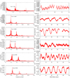 |
Fig. 4 Kepler long cadence light curves (right panel) and their power spectra (left panel). |
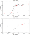 |
Fig. 5 Colour-period diagram of clusters NGC 6811 (upper panel) and NGC 6866 (lower panel). Exoplanet host stars are marked with red circles. |
7 Conclusions
Our main findings are summarised below.
-
We searched for inhomogeneities in the frequency of exoplanet occurrence on the scales of hundreds of parsecs. Data from Gaia and Kepler satellites were used for this purpose. We found statistically significant gradients of the uncorrected exoplanet frequency along the distance, Galactic longitude l = 90°, and height above the Galactic plane. We argue that these gradients are most probably caused by a single observational bias of undetected small planets around faint stars. When we corrected for this bias the gradients became statistically insignificant. Only the gradient of planet occurrence with distance for F stars remains significant at the 3σ level. Wedid not find any other significant gradients in the Cartesian, Galactocentric nor spherical coordinate systems. Consequently, apart from that one gradient, the spatial distribution of exoplanets in the Kepler field of view is compatible with a homogeneous one.
-
We searched for the inhomogeneities in the exoplanet frequency on the scales of tens of parsecs in the vicinity of open clusters based on Kepler and Gaia data. We do not find a significant difference in the exoplanet occurrence in the vicinity of the clusters.
-
The metallicity of our G star sample was found to increase with the Galactocentric radius and slightly decrease with the distance (at 2σ level). However, the metallicity of the F star sample increases slightly with the distance and y coordinate and drops with the Galactocentric radius and height above the Galactic plane. It means that it cannot be the reason for the drop of the exoplanet frequency around F stars with the distance since the exoplanet occurrence increases with the metallicity of the host star. However, this might have contributed to a drop of uncorrected exoplanet frequency around F stars with the height above the Galactic plane.
-
We discovered four exoplanet host star candidates which are members of the open cluster NGC 6811 (KIC 9655005, KIC 9533489, Kepler-66, Kepler-67). The last two had already been mentioned by Meibom et al. (2013).
-
We found two other promising exoplanet host star candidates which belong to the open cluster NGC 6866 (KIC 8396288, KIC 8331612). All these targets deserve further follow up using spectroscopy.
In the future, it might also be interesting to verify and expand this study using K2 (Howell et al. 2014), TESS (Ricker et al. 2014), or PLATO (Rauer et al. 2014) data in combination with the final Gaia data release.
Acknowledgements
We thank the anonymous referee for a very careful reading and many relevant suggestions. We are also grateful to Prof. Geza Kovacs, Prof. Nicolas Lodieu, and Jaroslav Merc for reading and useful comments on this manuscript. Our work was supported by the VEGA 2/0031/18 and Erasmus+ “Per aspera ad astra simul” (2017-1-CZ01-KA203-035562) projects. J.B. was also supported by the Slovak Research and Development Agency under the contract No. APVV-15-0458. This work has made use of data from the European Space Agency (ESA) mission Gaia (https://www.cosmos.esa.int/gaia), processed by the Gaia Data Processing and Analysis Consortium (DPAC, https://www.cosmos.esa.int/web/gaia/dpac/consortium). Funding for the DPAC has been provided by national institutions, in particular, the institutions participating in the Gaia Multilateral Agreement.
Appendix A: Spatial gradients of uncorrected exoplanet frequency
Appendix B: Spatial gradients of the metallicity
Gradients of metallicity based on all Kepler target stars (a volume-limited 16 mag sample) in spherical equatorial coordinates (r, α, δ).
Gradients of metallicity based on Kepler target stars (a volume-limited 16 mag sample) in coordinates (rg, z).
Gradients of metallicity based on Kepler target stars (a volume-limited 16 mag sample) in Cartesian coordinates (x, y, z).
Appendix C: Exoplanet candidates in the open clusters
Characteristics of the open clusters in the Kepler field of view.
Characteristics of our exoplanet host star candidates near NGC 6811 and NGC 5866.
Characteristics of our exoplanet host star candidates near NGC 6811 and NGC 6866.
References
- Agüeros, M. A., Bowsher, E. C., Bochanski, J. J., et al. 2018, ApJ, 862, 33 [NASA ADS] [CrossRef] [Google Scholar]
- Arenou, F., Luri, X., Babusiaux, C., et al. 2018, A&A, 616, A17 [Google Scholar]
- Balona, L. A., Joshi, S., Joshi, Y. C., & Sagar, R. 2013, MNRAS, 429, 1466 [NASA ADS] [CrossRef] [Google Scholar]
- Barnes, S. A. 2010, ApJ, 722, 222 [NASA ADS] [CrossRef] [Google Scholar]
- Barnes, S. A., Weingrill, J., Granzer, T., Spada, F., & Strassmeier, K. G. 2015, A&A, 583, A73 [NASA ADS] [CrossRef] [EDP Sciences] [Google Scholar]
- Barnes, S. A., Weingrill, J., Fritzewski, D., Strassmeier, K. G., & Platais, I. 2016, ApJ, 823, 16 [NASA ADS] [CrossRef] [Google Scholar]
- Bergemann, M., Ruchti, G. R., Serenelli, A., et al. 2014, A&A, 565, A89 [NASA ADS] [CrossRef] [EDP Sciences] [Google Scholar]
- Berger, T. A., Huber, D., Gaidos, E., & van Saders, J. L. 2018, ApJ, 866, 99 [NASA ADS] [CrossRef] [Google Scholar]
- Bognár, Z., Lampens, P., Frémat, Y., et al. 2015, A&A, 581, A77 [NASA ADS] [CrossRef] [EDP Sciences] [Google Scholar]
- Bonnell, I. A., Smith, K. W., Davies, M. B., & Horne, K. 2001, MNRAS, 322, 859 [NASA ADS] [CrossRef] [Google Scholar]
- Borucki, W. J., Koch, D., Basri, G., et al. 2010, Science, 327, 977 [NASA ADS] [CrossRef] [PubMed] [Google Scholar]
- Brown, T. M., Latham, D. W., Everett, M. E., & Esquerdo, G. A. 2011, AJ, 142, 112 [NASA ADS] [CrossRef] [Google Scholar]
- Buchhave, L. A., Latham, D. W., Johansen, A., et al. 2012, Nature, 486, 375 [NASA ADS] [Google Scholar]
- Burke, C. J., & Catanzarite, J. 2017, Planet Detection Metrics: Per-Target Detection Contours for Data Release 25, Technical report [Google Scholar]
- Burke, C. J., Christiansen, J. L., Mullally, F., et al. 2015, ApJ, 809, 8 [NASA ADS] [CrossRef] [Google Scholar]
- Cantat-Gaudin, T., Jordi, C., Vallenari, A., et al. 2018, A&A, 618, A93 [NASA ADS] [CrossRef] [EDP Sciences] [Google Scholar]
- Christiansen, J. L., Clarke, B. D., Burke, C. J., et al. 2015, ApJ, 810, 95 [NASA ADS] [CrossRef] [Google Scholar]
- Collier Cameron, A., Davidson, V. A., Hebb, L., et al. 2009, MNRAS, 400, 451 [NASA ADS] [CrossRef] [Google Scholar]
- Curtis, J. L., Vanderburg, A., Torres, G., et al. 2018, AJ, 155, 173 [NASA ADS] [CrossRef] [Google Scholar]
- Cutri, R. M., Skrutskie, M. F., van Dyk, S., et al. 2003, 2MASS All Sky Catalog of Point Sources (Washington, DC, USA: NASA) [Google Scholar]
- Deeming, T. J. 1975, Ap&SS, 36, 137 [NASA ADS] [CrossRef] [MathSciNet] [Google Scholar]
- Delorme, P., Cameron, A. C., Hebb, L., et al. 2011, ASP Conf. Ser., 448, 841 [NASA ADS] [Google Scholar]
- Dias, W. S., Alessi, B. S., Moitinho, A., & Lépine, J. R. D. 2002, A&A, 389, 871 [NASA ADS] [CrossRef] [EDP Sciences] [Google Scholar]
- Douglas, S. T., Agüeros, M. A., Covey, K. R., et al. 2016, ApJ, 822, 47 [NASA ADS] [CrossRef] [Google Scholar]
- Duong, L., Freeman, K. C., Asplund, M., et al. 2018, MNRAS, 476, 5216 [NASA ADS] [CrossRef] [Google Scholar]
- Errmann, R., Torres, G., Schmidt, T. O. B., et al. 2014, Astron. Nachr., 335, 345 [NASA ADS] [CrossRef] [Google Scholar]
- Esteban, C., & García-Rojas, J. 2018, MNRAS, 478, 2315 [NASA ADS] [CrossRef] [Google Scholar]
- Esteban, C., Fang, X., García-Rojas, J., & Toribio San Cipriano, L. 2017, MNRAS, 471, 987 [NASA ADS] [CrossRef] [Google Scholar]
- Fischer, D. A., & Valenti, J. 2005, ApJ, 622, 1102 [NASA ADS] [CrossRef] [Google Scholar]
- Fritzewski, D. J., Kitze, M., Mugrauer, M., et al. 2016, MNRAS, 462, 2396 [NASA ADS] [CrossRef] [Google Scholar]
- Fujii, M. S., & Hori, Y. 2019, A&A, 624, A110 [NASA ADS] [CrossRef] [EDP Sciences] [Google Scholar]
- Fulton, B. J., Petigura, E. A., Howard, A. W., et al. 2017, AJ, 154, 109 [NASA ADS] [CrossRef] [Google Scholar]
- Gaia Collaboration (Prusti, T., et al.) 2016, A&A, 595, A1 [NASA ADS] [CrossRef] [EDP Sciences] [Google Scholar]
- Gaia Collaboration (Brown, A. G. A., et al.) 2018, A&A, 616, A1 [NASA ADS] [CrossRef] [EDP Sciences] [Google Scholar]
- Gaidos, E., Mann, A. W., Rizzuto, A., et al. 2017, MNRAS, 464, 850 [NASA ADS] [CrossRef] [Google Scholar]
- Garai, Z., Pribulla, T., Hambálek, Ľ., et al. 2016, Astron. Nachr., 337, 261 [NASA ADS] [CrossRef] [Google Scholar]
- Hartman, J. D., Gaudi, B. S., Pinsonneault, M. H., et al. 2009, ApJ, 691, 342 [NASA ADS] [CrossRef] [Google Scholar]
- Howell, S. B., Sobeck, C., Haas, M., et al. 2014, PASP, 126, 398 [NASA ADS] [CrossRef] [Google Scholar]
- Jacobson, H. R., Friel, E. D., Jílková, L., et al. 2016, A&A, 591, A37 [NASA ADS] [CrossRef] [EDP Sciences] [Google Scholar]
- Khan, S., Miglio, A., Mosser, B., et al. 2019, A&A, 628, A35 [NASA ADS] [CrossRef] [EDP Sciences] [Google Scholar]
- Kipping, D. M., & Sandford, E. 2016, MNRAS, 463, 1323 [NASA ADS] [CrossRef] [Google Scholar]
- Kovács, G., Hartman, J. D., Bakos, G. Á., et al. 2014, MNRAS, 442, 2081 [NASA ADS] [CrossRef] [Google Scholar]
- Kraus, A. L., & Hillenbrand, L. A. 2007, AJ, 134, 2340 [NASA ADS] [CrossRef] [Google Scholar]
- Libralato, M., Nardiello, D., Bedin, L. R., et al. 2016, MNRAS, 463, 1780 [NASA ADS] [CrossRef] [Google Scholar]
- Lindegren, L., Hernández, J., Bombrun, A., et al. 2018, A&A, 616, A2 [NASA ADS] [CrossRef] [EDP Sciences] [Google Scholar]
- Livingston, J. H., Dai, F., Hirano, T., et al. 2018, AJ, 155, 115 [NASA ADS] [CrossRef] [Google Scholar]
- Mann, A. W., Gaidos, E., Vanderburg, A., et al. 2017, AJ, 153, 64 [Google Scholar]
- Mann, A. W., Vanderburg, A., Rizzuto, A. C., et al. 2018, AJ, 155, 4 [NASA ADS] [CrossRef] [Google Scholar]
- Mathur, S., Huber, D., Batalha, N. M., et al. 2017, ApJS, 229, 30 [NASA ADS] [CrossRef] [Google Scholar]
- Meibom, S., Barnes, S. A., Latham, D. W., et al. 2011, ApJ, 733, L9 [NASA ADS] [CrossRef] [Google Scholar]
- Meibom, S., Torres, G., Fressin, F., et al. 2013, Nature, 499, 55 [NASA ADS] [CrossRef] [Google Scholar]
- Mochejska, B. J., Stanek, K. Z., Sasselov, D. D., et al. 2005, AJ, 129, 2856 [NASA ADS] [CrossRef] [Google Scholar]
- Morton, T. D., Bryson, S. T., Coughlin, J. L., et al. 2016, ApJ, 822, 86 [NASA ADS] [CrossRef] [Google Scholar]
- Mulders, G. D., Pascucci, I., Apai, D., & Ciesla, F. J. 2018, AJ, 156, 24 [NASA ADS] [CrossRef] [Google Scholar]
- Narang, M., Manoj, P., Furlan, E., et al. 2018, AJ, 156, 221 [NASA ADS] [CrossRef] [Google Scholar]
- Netopil, M., Paunzen, E., Heiter, U., & Soubiran, C. 2016, A&A, 585, A150 [NASA ADS] [CrossRef] [EDP Sciences] [Google Scholar]
- Neuhäuser, R., Errmann, R., Berndt, A., et al. 2011, Astron. Nachr., 332, 547 [NASA ADS] [CrossRef] [Google Scholar]
- Pepper, J., Gillen, E., Parviainen, H., et al. 2017, AJ, 153, 177 [NASA ADS] [CrossRef] [Google Scholar]
- Petigura, E. A., Howard, A. W., Marcy, G. W., et al. 2017, AJ, 154, 107 [NASA ADS] [CrossRef] [Google Scholar]
- Petigura, E. A., Marcy, G. W., Winn, J. N., et al. 2018, AJ, 155, 89 [NASA ADS] [CrossRef] [Google Scholar]
- Quinn, S. N., White, R. J., Latham, D. W., et al. 2012, ApJ, 756, L33 [NASA ADS] [CrossRef] [Google Scholar]
- Radick, R. R., Thompson, D. T., Lockwood, G. W., Duncan, D. K., & Baggett, W. E. 1987, ApJ, 321, 459 [NASA ADS] [CrossRef] [Google Scholar]
- Rauer, H., Catala, C., Aerts, C., et al. 2014, Exp. Astron., 38, 249 [NASA ADS] [CrossRef] [Google Scholar]
- Ricker, G. R., Winn, J. N., Vanderspek, R., et al. 2014, SPIE Conf. Ser., 9143, 914320 [Google Scholar]
- Riess, A. G., Casertano, S., Yuan, W., et al. 2018, ApJ, 861, 126 [Google Scholar]
- Rizzuto, A. C., Mann, A. W., Vanderburg, A., Kraus, A. L., & Covey, K. R. 2017, AJ, 154, 224 [NASA ADS] [CrossRef] [Google Scholar]
- Rizzuto, A. C., Vanderburg, A., Mann, A. W., et al. 2018, AJ, 156, 195 [NASA ADS] [CrossRef] [Google Scholar]
- Rizzuto, A. C., Mann, A., Kraus, A. L., Vanderburg, A., & Ireland, M. 2019, AAS Meeting Abstracts, 233, 218.04 [Google Scholar]
- Sartoretti, P., Katz, D., Cropper, M., et al. 2018, A&A, 616, A6 [NASA ADS] [CrossRef] [EDP Sciences] [Google Scholar]
- Soubiran, C., Cantat-Gaudin, T., Romero-Gomez, M., et al. 2018, VizieR Online Data Catalog: J/A+A/619/A155 [Google Scholar]
- Stauffer, J., Rebull, L., Bouvier, J., et al. 2016, AJ, 152, 115 [NASA ADS] [CrossRef] [Google Scholar]
- van Sluijs, L., & Van Eylen, V. 2018, MNRAS, 474, 4603 [NASA ADS] [CrossRef] [Google Scholar]
- van Eyken, J. C., Ciardi, D. R., von Braun, K., et al. 2012, ApJ, 755, 42 [NASA ADS] [CrossRef] [Google Scholar]
- van Saders, J. L., Pinsonneault, M. H., & Barbieri, M. 2019, ApJ, 872, 128 [NASA ADS] [CrossRef] [Google Scholar]
- Vanderburg, A., Mann, A. W., Rizzuto, A., et al. 2018, AJ, 156, 46 [NASA ADS] [CrossRef] [Google Scholar]
- Wang, J., Xie, J.-W., Barclay, T., & Fischer, D. A. 2014a, ApJ, 783, 4 [NASA ADS] [CrossRef] [Google Scholar]
- Wang, J., Fischer, D. A., Xie, J.-W., & Ciardi, D. R. 2014b, ApJ, 791, 111 [NASA ADS] [CrossRef] [Google Scholar]
- Youdin, A. N. 2011, ApJ, 742, 38 [NASA ADS] [CrossRef] [Google Scholar]
- Zhu, W., Petrovich, C., Wu, Y., Dong, S., & Xie, J. 2018, ApJ, 860, 101 [NASA ADS] [CrossRef] [Google Scholar]
- Zinn, J. C., Pinsonneault, M. H., Huber, D., & Stello, D. 2019, ApJ, 878, 136 [NASA ADS] [CrossRef] [Google Scholar]
All Tables
Gradients of corrected exoplanet frequency for stars up to 16th magnitude in spherical equatorial coordinates (r, α, δ).
Gradients of corrected exoplanet frequency for stars up to 16th magnitude in cylindrical coordinates (rg, z).
Gradients of corrected exoplanet frequency for stars up to 16th magnitude in Cartesian coordinates (x, y, z).
Gradients of metallicity based on all Kepler target stars (a volume-limited 16 mag sample) in spherical equatorial coordinates (r, α, δ).
Gradients of metallicity based on Kepler target stars (a volume-limited 16 mag sample) in coordinates (rg, z).
Gradients of metallicity based on Kepler target stars (a volume-limited 16 mag sample) in Cartesian coordinates (x, y, z).
Characteristics of our exoplanet host star candidates near NGC 6811 and NGC 5866.
Characteristics of our exoplanet host star candidates near NGC 6811 and NGC 6866.
All Figures
|
Fig. 1 Location of exoplanet host stars (orange dots), Kepler target stars (grey dots), and open clusters (asterisks) in the Kepler field of view. Circles around some open clusters indicate the size of the inner cylinders used for statistics; see Sect. 5 for more details. |
| In the text | |
|
Fig. 2 Location of the Kepler target stars in the Galactic disc in (x, y) plane (upper panel) and (y, z) plane (lower panel). F, G, and K stars are highlighted with green, yellow, and red dots, respectively. The X-axis points to the Galactic centre. The direction of the Y-axis corresponds to the Galactic longitude of 90°. The three curves of constant Galactocentric radius are also plotted. |
| In the text | |
|
Fig. 3 Colour-magnitude diagram of clusters NGC 6811 (upper panel) and NGC 6866 (lower panel). Exoplanet host stars are marked with red circles. |
| In the text | |
|
Fig. 4 Kepler long cadence light curves (right panel) and their power spectra (left panel). |
| In the text | |
|
Fig. 5 Colour-period diagram of clusters NGC 6811 (upper panel) and NGC 6866 (lower panel). Exoplanet host stars are marked with red circles. |
| In the text | |
Current usage metrics show cumulative count of Article Views (full-text article views including HTML views, PDF and ePub downloads, according to the available data) and Abstracts Views on Vision4Press platform.
Data correspond to usage on the plateform after 2015. The current usage metrics is available 48-96 hours after online publication and is updated daily on week days.
Initial download of the metrics may take a while.