| Issue |
A&A
Volume 635, March 2020
|
|
|---|---|---|
| Article Number | A204 | |
| Number of page(s) | 7 | |
| Section | Planets and planetary systems | |
| DOI | https://doi.org/10.1051/0004-6361/201936390 | |
| Published online | 02 April 2020 | |
The role of disc torques in forming resonant planetary systems
Institut für Astronomie & Astrophysik, Universität Tübingen,
Auf der Morgenstelle 10,
72076
Tübingen,
Germany
e-mail: This email address is being protected from spambots. You need JavaScript enabled to view it.
Received:
27
July
2019
Accepted:
18
February
2020
Abstract
Context. The most accurate method for modelling planetary migration and hence the formation of resonant systems is using hydrodynamical simulations. Usually, the force (torque) acting on a planet is calculated using the forces from the gas disc and the star, while the gas accelerations are computed using the pressure gradient, the star, and the planet’s gravity, ignoring its own gravity. For a non-migrating planet the neglect of the disc gravity results in a consistent torque calculation while for a migrating case it is inconsistent.
Aims. We aim to study how much this inconsistent torque calculation can affect the final configuration of a two-planet system. We focus on low-mass planets because most of the multi-planetary systems, discovered by the Kepler survey, have masses around ten Earth masses.
Methods. Performing hydrodynamical simulations of planet–disc interaction, we measured the torques on non-migrating and migrating planets for various disc masses as well as density and temperature slopes with and without considering the self-gravity of the disc. Using this data, we found a relation that quantifies the inconsistency, used this relation in an N-body code, and performed an extended parameter study modelling the migration of a planetary system with different planet mass ratios and disc surface densities, to investigate the impact of the torque inconsistency on the architecture of the planetary system.
Results. Not considering disc self-gravity produces an artificially larger torque on the migrating planet that can result in tighter planetary systems. The deviation of this torque from the correct value is larger in discs with steeper surface density profiles.
Conclusions. In hydrodynamical modelling of multi-planetary systems, it is crucial to account for the torque correction, otherwise the results favour more packed systems. We examine two simple correction methods existing in the literature and show that they properly correct this problem.
Key words: hydrodynamics / methods: numerical / protoplanetary disks / planet–disk interactions
© ESO 2020
1 Introduction
Among thousands of known exoplanets, hundreds are in multi-planetary systems, and most have been discovered in the Kepler survey. One of the well-known properties of Kepler multi-planetary systems is the existence of pile-ups in the orbital period-ratio distribution just outside of some commensurabilities, specifically 2:1 and 3:2 (e.g. Fabrycky et al. 2014). Moreover, there are systems which have been shown to reside in resonance chains, such as Trappist-1 (Luger et al. 2017), GJ 876 (Millholland et al. 2018), Kepler-223 (Mills et al. 2016), and HD 40307 (Mayor et al. 2009). These observations demonstrate that there should be one or more mechanisms that place the planets into these fine-tuned configurations. One of the most promising mechanisms that is able to arrange planets in resonant configurations is planetary migration, that is the drift of a planet as a result of its gravitational interaction with the natal disc. There are numerous studies on modelling resonance configurations. This field was pioneered by Malhotra (1993) who showed that the migration of planets, owing to their interaction with either gas or planetesimal disc, can efficiently bring the planets into resonance. Forming resonant configurations requires convergent migration, meaning the outer planet should have larger migration rate than the inner planet, assuming the migration of both is towards the star. In convergent migration, the outer planet migrates faster, catches the inner one in a resonance, and then they continue their migration maintaining their orbital configuration (e.g. Lee & Peale 2002; Snellgrove et al. 2001). The final resonance configuration depends on how fast the outer planet crosses the resonance locations. The faster the outer planet migrates towards the inner planet, the closer the resonance configuration is. Therefore, in modelling of such systems, the migration speed of the planets is a key parameter.
Migration of a planet in a gas disc is determined by angular momentum exchange with the disc at the location of Lindblad and co-rotation resonances (see Kley & Nelson 2012, for a review). Ignoring the gas pressure and self-gravity, the resonances are located at those radii where the rotational frequency of the gas relative to the planet, Ω(r) − Ω(rp), matches a multiple of the epicyclic frequency in the disc κ(r). In other words, resonances are where the relation m(Ω(r) − Ω(rp)) = ±κ(r), where m is an integer, is satisfied. Whatever affects the gas angular frequency shifts the location of resonances and consequently changes the torque.
The angular velocity of a planet in a typical proto-planetary disc, which it is not massive and cold enough to be prone to gravitational instability, is dictated by the gravity from the central star and the disc. The angular velocity of the gas in the absence of the planet, Ω(r), is determined by the gravity of the star, the pressure gradient of the disc, and also the disc’s own gravity. In hydrodynamical modelling of planet-disc interaction, the third contribution – the disc’s self-gravity – is usually ignored for moderate disc masses of about minimum mass solar nebula (MMSN) in order to save the computation time. However, bymeans of analytical calculation (Pierens & Huré 2005) and numerical simulations (Baruteau & Masset 2008) it was shown that the torque on the planet would be more negative if the calculations of planet and gas angular velocities are inconsistent. This inconsistency occurs when the migrating planet feels both the star and the discbut the gas only feels the gravity of the star and not its own gravity. In such a condition, the term Ω(r) − Ω(rp) differs from the correct physical condition, when the disc self-gravity is included. This way of hydrodynamical simulations with migrating planets in a non-self-gravitating disc is very common in the literature (e.g. Snellgrove et al. 2001; Kley et al. 2004; Papaloizou & Szuszkiewicz 2005; Podlewska-Gaca & Szuszkiewicz 2011).
This is because it is not expected that a slightly faster migration affects the outcome significantly. However, in our attempt to model resonant planets with hydrodynamical simulations, we noticed that neglecting this effect produces unexpected resonant configurations and therefore, using the consistent calculation of the torque is essential. We note that the torques obtained from hydrodynamical simulations using a non-migrating planet in a non-self-gravitating disc are consistent because the angular velocity of the planet is enforced to be Keplerian. This means the planet only feels the star (e.g. Paardekooper et al. 2010, 2011). Therefore, these torques, which are widely used in one-dimensional (1D) or N-body models (e.g. Dittkrist et al. 2014; Bitsch et al. 2015; Brasser et al. 2018), are consistent.
There are several ways to obtain a consistent calculation of the torque for migrating planets while avoiding costly full self-gravitating simulations. One method, which was suggested by Baruteau & Masset (2008) and applied by Benítez-Llambay et al. (2016), is to use only the perturbed surface density for calculating the torque on the planet. This method removes the acceleration from the whole disc on the planet except for the non-axisymmetric perturbations induced by the planets such as spirals. Another method, also suggested by Baruteau & Masset (2008), includes the axi-symmetric part of the disc self-gravity in the calculation, assuming the contribution of the non-axi-symmetric part in the velocity of gas is negligible.
In this study we investigate how much an inconsistent torque calculation impacts the final configuration of a two-planet system. In Sect. 2, we initially examine how much the inconsistent torque differs from the correct torque for discs with varioussurface densities and temperature profiles. Then we examine two correction methods cited above and show that both perfectly fix the torque. In Sect. 3, we present the results of hydrodynamical simulations with two planets thathighlight the importance of torque correction and show that these two methods give similar results to their full self-gravitating counterparts. In Sect. 4, we first present a relation that gives the ratio of the correct torque to the inconsistent torque. This relation helps us to perform a parameter study using an N-body code to compare the outcome of two-planet simulations with the correct and inconsistent toque. Finally, we summarise our results in Sect. 5.
2 Migration of a single planet
In this section, we examine how much the torque on a migrating low-mass planet changes if we ignore the effect of disc self-gravity. We present the torque differences for various disc profiles and planetary masses as well as a comparison to the widely used torque formula of Paardekooper et al. (2011) (hereafter P11). These results are used later in Sect. 4 in the N-body simulations. Then we introduce and apply two correction methods, which already existed in the literature and we mention in Sect. 1, on the migrating torque. We compare the outcome of these methods with the non-migrating and full self-gravitating models.
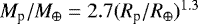
In this study, we focus only on low-mass planets, which do not perturb the disc greatly (i.e. do not open a gap), because most of the multi-planetary systems discovered by the Kepler space mission have Earth to mini-Neptune sizes. Using an exoplanet database1 and the mass-radius relation for low-mass planets by Wolfgang et al. (2016), we found that most of these planets have masses of about 5 M⊕ to 20 M⊕, which can be considered low mass for a typical disc around a solar-type star. Figure 1 shows the distribution of mass versus the orbital period ratio for each adjacent pair in Kepler multi-planet systems where the colour represents the mass of the inner planet. As the attached histogram to the colour bar shows, the mass of these planets is mostly between 5 M⊕ and 20 M⊕.
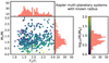 |
Fig. 1 Mass and orbital period ratios for two adjacent planets of Kepler multi-planetary systems. For the planets with unmeasured masses, the mass-radius relation |
2.1 Method and numerics
In order to measure the difference between migrating and non-migrating torques, we perform locally isothermal hydrodynamical simulations using the FARGO-ADSG code2 (Baruteau & Masset 2008). The disc surface density and temperature radial profiles follow power lows  and
and  , where r0 is the unit of length, chosen here to be 1 au. The temperature profile is related to the disc aspect ratio h through the sound speed (
 ) as
) as  where vK is Keplerian velocity, f is flaring index, and h0 = 0.05. Therefore, β = −2f + 1. We also respect the viscous equilibrium of the system by choosing the initial condition such that the mass accretion through the disc is constant Ṁ =3πνΣ. This imposes the condition α = 2f + 1∕2 for an alpha-viscosity model ν = ανcsH, that is used in this study. This constant Ṁ condition is important when a model needs to be simulated for a long time such that the viscous evolution of the disc might pollute the results otherwise. The disc, which spans from r = 0.3 to 2.5 and ϕ over the whole 2π, is divided by Nr × Ns = 512 × 1024 grid cells. The spacing is logarithmic in radial and equidistant in azimuthal direction. This resolution is sufficient for resolving the horseshoe region of planets with ten Earth-masses and larger. In cases with smaller planets, we have increased the resolution correspondingly. However, we did not find any considerable change in the results if this resolution is used for smaller planetary masses down to three Earth masses. The non-reflecting boundary condition is applied on the radial direction to damp the waves from the planet. The smoothing length of the for the gravitational potential is 0.6 H, where H is the disc scale height.
In those simulations which include the axi-symmetric part of the self-gravity or the disc’s full self-gravity, we consider the self-gravity smoothing length ɛSG equals to 0.6.
 |
Fig. 2 Scaled torque on a migrating (stars/dashed lines) and non-migrating (bullets/solid lines) planet as a function of surface density, Σ0 and planet mass M. The dotted lines indicate the partially saturated (P11) torques. These show the importance of disc self-gravity correction even for moderate surface density values. We continued the simulations with a non-zero vortensity gradient long enough to have the co-rotation torque established. |
2.2 Migrating versus non-migrating torque
In this section we study the torque acting on an embedded planet, non-migrating and migrating, for the case in which no disc self-gravity is considered. In the first step, we use the parameters α = 1.5 and f = 0.5 for the density and temperature slopes, which correspond to a locally isothermal disc with constant background vortensity. This guarantees that the torque on the planet is only generated by the Lindblad torque and avoids the complexity of the co-rotation torque (e.g. Masset et al. 2006; Paardekooper & Papaloizou 2008). In the next step, we alter the disc surface density and temperatureprofiles such that the gradient of inverse background vortensity becomes positive or negative, and we repeat the simulations again.
The planet mass varies between [3 − 20] M⊕ where M⊕ = 3 × 10⁻⁶ M⋆ is an Earth mass if M⋆, which is the mass of central star; also mass unit in our simulations equals to a solar mass. To see how much an inconsistent calculation (i.e. neglecting the effect of disc self-gravity) can alter the torque, we ran different models with various disc surface densities Σ0 =[10−6, 10−5, 10−4, 2 × 10⁻⁴, 3 × 10⁻⁴, 3 × 10⁻⁴], and compared the torque of a non-migrating planet to an identical simulation where the planet is allowed to migrate. The value of Σ0 =2 × 10⁻⁴ corresponds to the surface density at 1 au in the MMSN. The viscosity parameter is αν = 10−3.
The results are presented using the scaled torque3, Γ∕Γ0, where
 (1)
(1)
is the torque normalisation which is calculated at the actual location of the planet, rp, where q is the planet-to-star mass ratio and Ωp Keplerian angular velocity at rp.
Figure 2 shows the scaled torque for three disc models with the specified profiles. Each point represents the obtained torque for different surface density Σ0 and planetary mass M. The torques are measured after the planet settled completely in the disc and its torque reached a constant value. This relaxation time is 60 orbits for the zero vortensity model and 700 orbits for the other two. The theoretical torques, dotted lines, are calculated using Eqs. (5), (50)–(53) in P11 with Pχ = 0 (meaning that we assume thermal diffusivity is infinite in a locally isothermal disc) and taking into account the effect of smoothing length from Paardekooper et al. (2010). In all three panels, the normalised torque on a non-migrating planet does not depend on the value of surface density. On the contrary, the torque on a migrating planet can increase by a factor 1.5 compared to the non-migrating value as the surface density quadruples. In the middle panel, the torque is only Lindblad and all lines for non-migrating cases almost overlap with the theoretical cases. The slightly smaller torque of the 20 M⊕ planet is because of a very shallow partial gap around the planet. In the other two panels, the non-zero background vortensity gradient creates a contribution from the co-rotation torque that depends on the horseshoe size and thereupon on the mass of the planet. In these cases, the P11 formulae give similar values which are in agreement with the non-migrating torques with the maximum error of about 20% for the highest planetary mass.
Except for the model with constant background vortensity, we might wonder if the difference between the migrating and non-migrating torque can be due to the dynamical co-rotation torque (Paardekooper 2014), which is a possible component of the co-rotation torque that arises from the vortensity gradient created in the horseshoe region because of the migration of the planet. For example if a low-mass planet migrates a long distance in the disc while preserving its initial vortensity in the horseshoe region, the dynamical torque can be significant. In our models, neither the planet migrates a long distance (maximum 0.24 length unit) nor is the viscosity so low to retain the initial vortensity. The conditions given in Paardekooper (2014) can help us to check whether the dynamical torque has a significantrole in our simulations or not. Our set-up falls into his second condition because (a) the variable  (his Eq. (20)) is larger than unity for our lowest planetary mass and highest surface density, (b) our viscosity timescale over the horseshoe region is smaller than the migration time scale τν < τmig, (c) and mc τν∕τmig < 1. Therefore, the dynamical torque cannot be significant in our models. However, in long simulations for modelling of the resonant planets, thiscomponent may influence the results.
Another point deduced from Fig. 2 is that the difference between the non-migrating and migrating torque is much smaller for the model with positive co-rotation torque, namely Σ ∝ r−0.5 and h = 0.05. Therefore, we expect that using an inconsistent torque for this profile does not make a big difference when simulating resonant planets. We investigate this issue in Sect. 4.
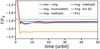 |
Fig. 3 Time evolution of the torque acting on a 10 Earth-mass planet in a disc with vanishing vortensity gradient for migrating and non-migrating planets. Both of the correcting methods fix the migrating torque perfectly and return it to the non-migrating value which is identical to the full self-gravitating torque (the purple line). The horizontal line denoted with P11 shows the theoretical Lindblad torque. |
2.3 Correcting the migrating torque
In this section, we test the two previously mentioned methods for correcting the torque (force) on a migrating planet in hydrodynamical studies and compare the results with the torque on a non-migrating planet as well as with the torque in a full self-gravitating simulation. For a consistent calculation of the torque, planet and gas velocities should be both computed in the same way. This can be achieved by either including or excluding the disc self-gravity simultaneously for both. Therefore, two methods aresuggested in the literature:
The first method excludes the disc self-gravity by using only the perturbed gas density for calculating the disc force on the planet. In this method, the azimuthally averaged surface density is subtracted from each cell prior to the force calculation (Benítez-Llambay et al. 2016). Therefore, the acceleration from the whole disc on the planet vanishes except where is azimuthally perturbed and the velocity of the planet remains close to Keplerian.
The second method including the axi-symmetric part of the disc self-gravity as a source term in the gas momentum equation as suggestedby Baruteau & Masset (2008). In this method, the gas velocities are computed with the same approach as the gravitational forces on the planet.
Figure 3 shows the non-migrating, inconsistent migrating, corrected migrating torques, and the torque calculated taking the full self-gravity of the disc into account for a ten Earth-mass planet in a disc with zero background vortensity and Σ0 =2 × 10⁻⁴. Figure 4 demonstrates the migration and eccentricity damping for a circular and an eccentric planet of the same mass and disc as in Fig. 3. The symbols denote the correction methods and the inconsistent torque, while the line refers to thefull self-gravity model. These two show that both of these methods remedy the torque perfectly and either of them must be applied in hydrodynamical simulations of multi-planets, in particular when considering the formation of resonant configurations, which depends delicately on the differential migration speed of the two planets. Interestingly, eccentricity damps with the same rate in the all models.
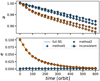 |
Fig. 4 Semi-major axis a and eccentricity e evolution of a planet with e0 = 0 and 0.1 for the correct, inconsistent, and full self-gravity torques. The results of both methods excellently overlap with the full self-gravity model. |
3 Tighter resonances with inconsistent torque
One common way to study resonant configurations is using an inner planet that is trapped or has slower migration together with an outer planet that migrates faster and catches the inner planet in a resonance (e.g. Kley et al. 2004; Papaloizou & Szuszkiewicz 2005; Podlewska-Gaca & Szuszkiewicz 2011; Paardekooper et al. 2013; Cui et al. 2019). We used this approach and constructed a planetary trap by increasing the disc viscosity in the inner part of the disc. Accordingly, a density maximum is created with a very steep positive density gradient that can trap the planets. Then, we planted two planets with masses Mi = 10 M⊕ and Mo = 20 M⊕ in the disc andallowed them to migrate. Subscripts “i” and “o” refer to the inner and outer planet, respectively. Three simulations with identical initialisation were run except that we used the corrected torque in one of these simulations, the inconsistent torque in the second, and full self-gravitating calculation in the third one to examine what happens to the resonant configuration when as inconsistent torque is used.
The upper panel in Fig. 5 shows the evolved surface density and the positions of the planets after the planets have been locked into resonance. This profile is almost time-independent and very similar in all three simulations. The lower panel of Fig. 5 compares the orbital period ratio of the outer to inner planet between the models. The final location of these planets are also denoted in the upper panel with the corresponding colours. This figure clearly signifies the role of correction. While the inner planet is trapped in all models at the zero torque location (Masset et al. 2006), the outer planet migrates more inwards in the model with inconsistent torque than that with the correct torque, which produced the same final configuration as the model with full self-gravity. This can be explained easily using the results in Sect. 2. Because the inconsistent torque is larger than the correct torque, the planet migrates faster and crosses the wider resonances even for the low surface densities as we used in this work. This is why the outer planet in the model with inconsistent torque was able to pass through more resonances until it finally reached the 5:4 commensurability. On the other hand, the model with correct torque has been stopped in the wider 4:3 resonance. As a result, an incorrect torque treatment (i.e. not considering disc self-gravity at all) leads to capturing closer resonances, which might impact the stability of the system.
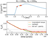 |
Fig. 5 Resonant capture of two planets (with 10 and 20 MEarth) at a planet trap located at 1 au obtained by hydrodynamical simulations. Orange, green, and red refer to the simulations with inconsistent, corrected, and full self-gravitating torques, respectively. Upper panel: final surface density and planet positions. Lower panel: time evolution of the period ratio (outer to inner planet) of the two planets. |
4 Under what condition can an inconsistent torque be troublesome
Because the migration rate of a planet depends directly on its mass and the disc surface density, we investigate in this section under what conditions ignoring the torque (resp. self-gravity) correction can be risky. Although the migration rate depends inversely on the disc aspect ratio, we do not study this parameter because for small aspect ratios, even moderate planetary masses can open a partial gap and enter into a different migration regime which is not within the scope of this study. A parameter study is needed to find out for what values of disc surface densities and planetary masses the final resonance configuration depends strongly on the torque correction. However, performing such a parameter study using hydrodynamical simulation would be numerically expensive. To circumvent this issue, we use N-body simulations which are much faster. However, we first need to know how much the results of N-body simulations agree with hydrodynamical simulations for correct and inconsistent torque.
4.1 N-body versus hydrodynamical simulations
Among the models in Sect. 2.2, the disc with 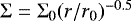 and constant aspect ratio shows the least difference between the migrating and non-migrating torques. Therefore, this model can be considered as the most conservative. If we see considerable differences in the final configurations, the case for other disc models would be even worse. Henceforth, we consider this model with Σ0 =2 × 10⁻⁴, corresponding to 1777 [g cm−2] for a solar-mass star and the length unit of 1 au, and h = 0.05. We place two planets with masses Mi = Mo = 10 M⊕ just out of 2:1 resonance and allow the system to evolve. The set-up for the hydrodynamical simulations is otherwise identical to Sect. 2.1.
The N-body simulations were carried out via the REBOUND code4 (Rein & Liu 2012) with the IAS15 integrator (Rein & Spiegel 2015), and identical planet initialisation as our hydrodynamical simulations. Migration of the planets is modelled using the torque formulae in P11 along with the correction factors for the eccentricity of the planet as in Cresswell & Nelson (2008) for Lindblad and Fendyke & Nelson (2014) for co-rotation torque. We followed the approach of Papaloizou (2011) to convert the torques to the planet acceleration. Because we also want to simulate models with inconsistent torque, following Baruteau & Masset (2008), we fitted a function to the data in Sect. 2.2 that gives us the ratio of the inconsistent torques Γmig to the non-migrating torques Γfix. This function reads
 (2)
(2)
where Q is the Toomre parameter at the location of the planet5. Therefore, for modelling the inconsistent torque in the N-body simulations, we apply this relation on the total torque from P11.
For the disc and the planetary masses in this work, we expect that the planets keep their initial period ratio without diverging or converging. When two inwardly migrating planets converge, the outer planet has a larger migration rate than the inner. In other words, ȧo > ȧi, where a is the semi-major axis of the planet. The migration rate of a non-eccentric planet is related to the torque as
 (3)
(3)
where the torque Γ is determined by (a) the disc surface density and temperature slopes − α and − β, which are constant in our models; and (b) Γ0 ∝ q2a−α+1−2f (see Eq. (1)), which varies as the planet migrate. Therefore, the latter determines if the migration of our planets diverges or converges. Applying the condition of viscous equilibrium gives Γ0 ∝ q2a−2α+3∕2, and substituting Γ0 in Eq. (3) gives
 (4)
(4)
The convergence condition then is written as
 (5)
(5)
For equal mass planets, this condition is satisfied only if α > 0.5. Therefore, for our set-up, both migration timescales are equal and, on paper, we expect they neither converge nor diverge. However, the condition in a hydrodynamical simulation would be different owing to the planet-spiral (Baruteau & Papaloizou 2013) or planet–planet interactions.
Figure 6 shows the orbital period ratio of our planets for four hydrodynamical and three N-body simulations, all of which are initialised identically. Three hydrodynamical simulations in which we used either the correct torque or ran with full self-gravity agree well and do not show a considerable divergence or convergence during the running time. In contrast, the hydrodynamical simulation with the inconsistent torque diverges into 2:1 resonance. This is the result that is also produced by the N-body simulation where we used Eq. (2) to mimic the inconsistent torques. In contrast to the correct hydrodynamical simulations, the N-body simulation with the correct torque shows convergence. This behaviour happens when we apply the eccentricity correction on the Lindblad torques. A slight eccentricity of the outer planet increases the torque such that they converge by time. Although the N-body gives convergent migration compared to the hydrodynamical simulation, it is slower than that with the inconsistent torque and we can still use the N-body simulations for the parameter study, keeping in mind that the results underestimate the difference between the models with inconsistent and correct torque. If we see a notable difference, it would be even larger when using hydrodynamical simulations.
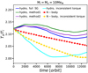 |
Fig. 6 Orbital period ratio of two equal mass planets in a disc with Σ ∝ r−0.5 and h = 0.05 using an N-body and a hydrodynamical code. The inconsistent torques in the N-body simulation has been computed based on the data in Sect. 2.2; see Eq. (2). |
4.2 Parameter study
Inspired by the Kepler data in Fig. 1, we focused on planets with masses between [1– 20] M⊕ and an outer-to-inner planet mass ratios between [0.8–2]. Surface density is varied as Σ0 ∈ [1–4] × 10−4, from half to twice of the MMSN’s value. We initialised the system as in Sect. 4.1 and allowed it to evolve for 10 000 yr using the N-body code. The results are summarised in Fig. 7. The left panels, which represent the results of the simulations with correct torques, show that all models with mass ratios below 1.1 do not converge, regardless of the surface density values. The migration only converges when the outer planet becomes more massive than the inner planet. On the contrary, the models with inconsistent torques can produce more packed systems. This can be understood by comparing the location of the marked contours, which show some commensurabilities. For example, equal mass planets reach the 2:1 resonance for higher surface densities, while the correct torque simulations do not predict reaching to 2:1 resonance. Considering the N-body results favour a smaller difference between the two sets, we can conclude that applying the torque correction in hydrodynamical simulations would produce wider configurations.
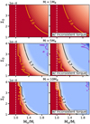 |
Fig. 7 Orbital period ratio of the outer to inner planet for models with correct torque (left column) and those with inconsistent torque (right column) as a function of planet mass ratio and surface density. Commensurabilities are indicated by coloured lines: 2:1 by yellow, 5:3 by black, and 3:2 by purple. Visibly, using inconsistent torque can produce more packed configurations. |
5 Summary
Migration of planets is the result of gravitational interaction between the planets and their natal disc. A planet plays the role of a perturber in a disc and creates spiral arms as the consequence of its interaction with the gas at Lindblad resonances. Location of these resonances is a function of relative angular velocity of the gas to the planet, namely Ω(r) − Ω(rp). In order to calculate the planetary migration correctly, the computation of these two velocities should be consistent, meaning that the disc gravity should be either included or excluded in calculating the force acting on both, the gas and planet. However, this is often ignored in hydrodynamical simulations when the disc mass is low, and the disc force only acts on the planet. We showed in this work that because of this inconsistent calculation, a slightly larger torque can make more packed planetary systems and even fake resonant configurations. We examined two suggested methods in the literature for correcting the torque:
The first method used only the surface density perturbation to calculate the force from disc on the planet while ignoring the disc self-gravity (Benítez-Llambay et al. 2016; Baruteau & Masset 2008). In this method, the disc gravity, except from the perturbed gas, is excluded from calculations.
The second method includes the axisymmetric part of the disc self-gravity in the gas momentum equation (Baruteau & Masset 2008). In this way, the disc gravity is included in calculation of both planet and gas. A convenient numerical procedure is given in Kley (1996).
We showed that both of these methods give identical results as the models with full self-gravity. Considering that they take similar computational time, one of these corrections must be applied in hydrodynamical modelling of planetary systems, otherwise, the results would not be very reliable. In this case, the inclusion of axisymmetric disc self-gravity is physically more realistic andcan be generalised to full self-gravity if required.
We examined this issue for low-mass planets in the mass range of Kepler planets through customised N-body simulations. For this we used the most conservative disc set-up with a density slope for which the differences between consistent and inconsistent forces were minimal, hence we expect an even stronger effect for other situations. Since base of the calculations and the physics is the same for higher mass planets, we expect that this issue affects the migration of higher mass planets as well, but may be less pronounced owing to the gap opening.
We would like to emphasise that the calculation of popular torque formulae, which are widely used in N-body simulations, are consistent because in those studies the planet is enforced to move Keplerian while the gas self-gravity is ignored. Such a condition, as we explained before, is consistent. There is also another method of calculation in the literature that the planet is forced to migrate with a given migration rate and then the torque on the planet is measured (Duffell et al. 2014; Meru et al. 2019). We find that this method is also consistent since the velocity of the planet is not calculated directly from the gas but is set actually by hand. Our warning refers mostly to the models in which the migration of the planet is calculated directly through its gravitational interaction by the disc.
Finally, we would like to point out that only full hydrodynamical simulations including self-gravity corrections give reliable results because additional effects caused by gravitational interaction with the spiral arms produced by the planets play a role. These are difficult to capture using N-body simulations.
Acknowledgements
We acknowledge the support of the DFG priority program SPP 1992 “Exploring the Diversity of Extrasolar Planets under grant KL 650/27”. The authors also acknowledge support by the state of Baden-Württemberg through bwHPC. We would like to thank A. Crida for the stimulating discussion and the anonymous referee for her/his comments which helped improving the study.
References
- Baruteau, C., & Masset, F. 2008, ApJ, 678, 483 [NASA ADS] [CrossRef] [Google Scholar]
- Baruteau, C., & Papaloizou, J. C. B. 2013, ApJ, 778, 7 [NASA ADS] [CrossRef] [Google Scholar]
- Benítez-Llambay, P., Ramos, X. S., Beaugé, C., & Masset, F. S. 2016, ApJ, 826, 13 [NASA ADS] [CrossRef] [Google Scholar]
- Bitsch, B., Johansen, A., Lambrechts, M., & Morbidelli, A. 2015, A&A, 575, A28 [NASA ADS] [CrossRef] [EDP Sciences] [Google Scholar]
- Brasser, R., Matsumura, S., Muto, T., & Ida, S. 2018, ApJ, 864, L8 [NASA ADS] [CrossRef] [Google Scholar]
- Cresswell, P., & Nelson, R. P. 2008, A&A, 482, 677 [NASA ADS] [CrossRef] [EDP Sciences] [Google Scholar]
- Cui, Z., Papaloizou, J. C. B., & Szuszkiewicz, E. 2019, ApJ, 872, 72 [NASA ADS] [CrossRef] [Google Scholar]
- Dittkrist, K. M., Mordasini, C., Klahr, H., Alibert, Y., & Henning, T. 2014, A&A, 567, A121 [NASA ADS] [CrossRef] [EDP Sciences] [Google Scholar]
- Duffell, P. C., Haiman, Z., MacFadyen, A. I., D’Orazio, D. J., & Farris, B. D. 2014, ApJ, 792, L10 [NASA ADS] [CrossRef] [Google Scholar]
- Fabrycky, D. C., Lissauer, J. J., Ragozzine, D., et al. 2014, ApJ, 790, 146 [NASA ADS] [CrossRef] [Google Scholar]
- Fendyke, S. M., & Nelson, R. P. 2014, MNRAS, 437, 96 [NASA ADS] [CrossRef] [Google Scholar]
- Kley, W. 1996, MNRAS, 282, 234 [NASA ADS] [CrossRef] [Google Scholar]
- Kley, W., & Nelson, R. P. 2012, ARA&A, 50, 211 [NASA ADS] [CrossRef] [Google Scholar]
- Kley, W., Peitz, J., & Bryden, G. 2004, A&A, 414, 735 [NASA ADS] [CrossRef] [EDP Sciences] [Google Scholar]
- Lee, M. H., & Peale, S. J. 2002, ApJ, 567, 596 [NASA ADS] [CrossRef] [Google Scholar]
- Luger, R., Sestovic, M., Kruse, E., et al. 2017, Nat. Astron., 1, 0129 [Google Scholar]
- Malhotra, R. 1993, Nature, 365, 819 [CrossRef] [Google Scholar]
- Masset, F. S., Morbidelli, A., Crida, A., & Ferreira, J. 2006, ApJ, 642, 478 [NASA ADS] [CrossRef] [Google Scholar]
- Mayor, M., Udry, S., Lovis, C., et al. 2009, A&A, 493, 639 [NASA ADS] [CrossRef] [EDP Sciences] [Google Scholar]
- Meru, F., Rosotti, G. P., Booth, R. A., Nazari, P., & Clarke, C. J. 2019, MNRAS, 482, 3678 [NASA ADS] [CrossRef] [Google Scholar]
- Millholland, S., Laughlin, G., Teske, J., et al. 2018, AJ, 155, 106 [NASA ADS] [CrossRef] [Google Scholar]
- Mills, S. M., Fabrycky, D. C., Migaszewski, C., et al. 2016, Nature, 533, 509 [NASA ADS] [CrossRef] [Google Scholar]
- Paardekooper,S. J. 2014, MNRAS, 444, 2031 [NASA ADS] [CrossRef] [Google Scholar]
- Paardekooper,S. J., & Papaloizou, J. C. B. 2008, A&A, 485, 877 [NASA ADS] [CrossRef] [EDP Sciences] [Google Scholar]
- Paardekooper,S. J., Baruteau, C., Crida, A., & Kley, W. 2010, MNRAS, 401, 1950 [NASA ADS] [CrossRef] [Google Scholar]
- Paardekooper,S. J., Baruteau, C., & Kley, W. 2011, MNRAS, 410, 293 [NASA ADS] [CrossRef] [Google Scholar]
- Paardekooper,S.-J., Rein, H., & Kley, W. 2013, MNRAS, 434, 3018 [NASA ADS] [CrossRef] [Google Scholar]
- Papaloizou, J. C. B. 2011, Celest. Mech. Dyn. Astron., 111, 83 [NASA ADS] [CrossRef] [Google Scholar]
- Papaloizou, J. C. B., & Szuszkiewicz, E. 2005, MNRAS, 363, 153 [NASA ADS] [CrossRef] [MathSciNet] [Google Scholar]
- Pierens, A., & Huré, J. M. 2005, A&A, 433, L37 [NASA ADS] [CrossRef] [EDP Sciences] [Google Scholar]
- Podlewska-Gaca, E., & Szuszkiewicz, E. 2011, MNRAS, 417, 2253 [NASA ADS] [CrossRef] [Google Scholar]
- Rein, H., & Liu, S. F. 2012, A&A, 537, A128 [NASA ADS] [CrossRef] [EDP Sciences] [Google Scholar]
- Rein, H., & Spiegel, D. S. 2015, MNRAS, 446, 1424 [NASA ADS] [CrossRef] [Google Scholar]
- Snellgrove, M. D., Papaloizou, J. C. B., & Nelson, R. P. 2001, A&A, 374, 1092 [NASA ADS] [CrossRef] [EDP Sciences] [Google Scholar]
- Wolfgang, A., Rogers, L. A., & Ford, E. B. 2016, ApJ, 825, 19 [NASA ADS] [CrossRef] [Google Scholar]
We note that since we only use the scaled torque in this paper, the words torque and scaled torque might be used interchangeably.
Available at http://github.com/hannorein/rebound
Note that the fitting in Baruteau & Masset (2008) has been done over Qh. In this study, since we do not vary the value of h at the location of the planet, it has been enclosed in the coefficient.
All Figures
|
Fig. 1 Mass and orbital period ratios for two adjacent planets of Kepler multi-planetary systems. For the planets with unmeasured masses, the mass-radius relation |
| In the text | |
|
Fig. 2 Scaled torque on a migrating (stars/dashed lines) and non-migrating (bullets/solid lines) planet as a function of surface density, Σ0 and planet mass M. The dotted lines indicate the partially saturated (P11) torques. These show the importance of disc self-gravity correction even for moderate surface density values. We continued the simulations with a non-zero vortensity gradient long enough to have the co-rotation torque established. |
| In the text | |
|
Fig. 3 Time evolution of the torque acting on a 10 Earth-mass planet in a disc with vanishing vortensity gradient for migrating and non-migrating planets. Both of the correcting methods fix the migrating torque perfectly and return it to the non-migrating value which is identical to the full self-gravitating torque (the purple line). The horizontal line denoted with P11 shows the theoretical Lindblad torque. |
| In the text | |
|
Fig. 4 Semi-major axis a and eccentricity e evolution of a planet with e0 = 0 and 0.1 for the correct, inconsistent, and full self-gravity torques. The results of both methods excellently overlap with the full self-gravity model. |
| In the text | |
|
Fig. 5 Resonant capture of two planets (with 10 and 20 MEarth) at a planet trap located at 1 au obtained by hydrodynamical simulations. Orange, green, and red refer to the simulations with inconsistent, corrected, and full self-gravitating torques, respectively. Upper panel: final surface density and planet positions. Lower panel: time evolution of the period ratio (outer to inner planet) of the two planets. |
| In the text | |
|
Fig. 6 Orbital period ratio of two equal mass planets in a disc with Σ ∝ r−0.5 and h = 0.05 using an N-body and a hydrodynamical code. The inconsistent torques in the N-body simulation has been computed based on the data in Sect. 2.2; see Eq. (2). |
| In the text | |
|
Fig. 7 Orbital period ratio of the outer to inner planet for models with correct torque (left column) and those with inconsistent torque (right column) as a function of planet mass ratio and surface density. Commensurabilities are indicated by coloured lines: 2:1 by yellow, 5:3 by black, and 3:2 by purple. Visibly, using inconsistent torque can produce more packed configurations. |
| In the text | |
Current usage metrics show cumulative count of Article Views (full-text article views including HTML views, PDF and ePub downloads, according to the available data) and Abstracts Views on Vision4Press platform.
Data correspond to usage on the plateform after 2015. The current usage metrics is available 48-96 hours after online publication and is updated daily on week days.
Initial download of the metrics may take a while.