| Issue |
A&A
Volume 634, February 2020
|
|
|---|---|---|
| Article Number | A60 | |
| Number of page(s) | 15 | |
| Section | Planets and planetary systems | |
| DOI | https://doi.org/10.1051/0004-6361/201937224 | |
| Published online | 07 February 2020 | |
Orbit classification in exoplanetary systems
1
Department of Physics, School of Science, Aristotle University of Thessaloniki,
541 24
Thessaloniki,
Greece
e-mail: This email address is being protected from spambots. You need JavaScript enabled to view it.
2
Department of Astronomy, Eötvös University,
Pázmány Péter sétány 1/A,
1117
Budapest,
Hungary
e-mail: This email address is being protected from spambots. You need JavaScript enabled to view it.
3
Nonlinear Analysis and Applied Mathematics (NAAM)-Research Group, Department of Mathematics, Faculty of Science, King Abdulaziz University,
PO Box 80203,
Jeddah
21589,
Saudi Arabia
e-mail: This email address is being protected from spambots. You need JavaScript enabled to view it.
Received:
30
November
2019
Accepted:
12
January
2020
Abstract
The circular version of the restricted three-body problem, along with the method of grid classification are used to determine the character of the trajectories of a test particle, which move in a binary exoplanetary system. The binary system can be either a parent star-exoplanet or an exoplanet–exoplanet or exomoon, while the test particle is considered to be an asteroid or comet, a space probe, or even a small exomoon in the case where the primary body is a star. By using modern two-dimensional color maps, we succeeded in classifying the starting conditions and distinguishing between bounded, escaping, and collision type of motion for the test particle. Furthermore, in the case of bounded regular motion, we further classify the starting conditions by considering their geometry (revolving around one or both main bodies) and orientation (prograde or retrograde, with respect to a rotating coordinate system of the primaries). For the initial setup of the test particle we consider two starting conditions: the launch from pericenter or apocenter. The final states are qualitatively visualized through two-dimensional basin diagrams. This approach allowed us to systematically investigate and extract dynamical information on the dependency of the test particle final state as a function of the particle’s initial semi-major axis and eccentricity for a given primary and secondary mass ratio. Finally, we applied the restricted three-body model on several exoplanetary systems with observed mass-ratios and studied the dynamical behavior of a test-mass.
Key words: methods: numerical / celestial mechanics
© ESO 2020
1 Introduction
There is no doubt that nowadays the topic of exoplanets is one of the most active and interesting fields in Astronomy. According to NASA Exoplanet Archive1, there are more than 4100 confirmed exoplanets in 3067 exosolar systems, of which 671 have more than one exoplanet. Therefore, these new findings strongly suggest that our Solar System should not be considered as a typical planetary system, but more as an exception. Consequently, the intervals regarding the typical numerical values of the orbital eccentricity, the semi-major axis, as well as the mass ratio of the planetary systems should be revised.
It is observed for many exoplanets that the corresponding masses are very similar to the masses of the planets of our Solar System. The main difference is that some exoplanets follow high eccentric orbits, while they circulate relatively close to their parent stars. The majority of the exoplanets move on planar circular orbits, with an orbital period of 8–12 days, while they have a Jovian mass value. On the other hand, only a small minority of exoplanets follow trajectories with high eccentricity and/or inclination (e.g., HD 43197b, HD 45350b, HD 80606b, HD 96167b, GJ 317c, etc.). Interestingly, in the case where multiple exoplanets exist in an exosolar system, they appear to be locked in mean-motion resonances (MMRs). In particular, a significant fraction of them move in 2:1 resonance (e.g., HD 73456, HD 82943, HD 128311), while the other types of resonances are also possible that is, 3:1 (e.g., HD 60532), 3:2 (e.g., HD 45364), 4:1 (e.g., HD 108874), 4:3, and 5:2 (see e.g., Antoniadou 2016; Campanella 2011; Campanella et al. 2013; Correia et al. 2010; Couetdic et al. 2010; Laskar & Correia 2004; Goździewski et al. 2006; Lovis et al. 2011; Rein et al. 2010).
The circular version of the restricted three-body problem is very useful, in its simplicity, for describing the motion in exoplanetary systems. For the case where the distance between the two bodies is large enough, that is outside the Hill’s sphere of influence we have the one-dimensional models (1D), which were developed to describe the averaged dynamics in the coplanar case (see e.g., Érdi 1977; Robutel & Pousse 2013). Obviously, in the scenario that involves eccentric and/or inclined motion, the orbital dynamics in phase space is much more complicated due to the higher number of degrees of freedom. For example, in the eccentric case, additional coorbital configurations emerge (see e.g., Mikkola et al. 2006; Namouni 1999; Pousse et al. 2017; Sidorenko et al. 2014), while in the inclined case we have new retrograde coorbital configurations (Morais & Namouni 2013). The coorbital model has been applied in many studies to search for Trojan exoplanets (see e.g., Érdi & Sándor 2005; Funk et al. 2012; Hippke & Angerhausen 2015; Laughlin & Chambers 2002; Leleu et al. 2017; Schwarz et al. 2012).
In recent years, several studies have been devoted to demystifying the dynamics of exoplanetary systems by using various dynamical models and numerical techniques (see e.g., Antoniadou 2016; Antoniadou & Voyatzis 2014, 2016; Ferraz-Mello et al. 2006; Hadjidemetriou 2006; Henrard & Libert 2008; Lee 2004; Michtchenko et al. 2006; Voyatzis 2008). Most of these works attempt to either distinguish between order and chaos, or to present a new numerical technique to detect nonlinear dynamics or study specific resonant configurations considering families of periodic orbits. Conversely, in our work we apply the computational methods introduced and applied in Nagler (2004, 2005) in order to perform a thorough and systematic taxonomy of the staring conditions of the test particle. Following this technique allows us to gain insight into different types of phase-space basins (corresponding to bounded, escaping, and collision motion) on two-dimensional maps. For the starting conditions of the massless particle, the approach used in Érdi et al. (2012) is adopted, thus considering only pericentric and apocentric launching.
The article is organized according to the following layout: Sect. 2 contains the mathematical formulation of the dynamical system, followed by Sect. 3, where we describe the computational methodology, used for the taxonomy of the trajectories. The main outcomes of our analysis are analyzed in Sect. 4 and our paper ends with the main conclusions given in Sect. 5.
2 Mathematical formulation of the dynamical system
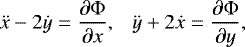
In our analysis, we shall use the model of the restricted three-body problem, according to which a (massless) test particle moves under the gravitational influence of two bodies with considerably larger masses. These two bodies B1 and B2 (with masses m1 and m2), known as the primary and secondary respectively, move on a planar and circular trajectory around their common center of gravity. It should be noted, that the plane of motion of B1 and B2 coincides with that of the massless particle m. Then, the on-plane motion of the test particle is governed, according to the equations of motion formulated in a co-rotating reference frame (see e.g., Murray & Dermott 1999)
 (1)
(1)
where
 (2)
(2)
is the negative effective potential, and where x1 = −μ and x2 = 1 − μ are the positions of two main bodies on the x-axis. In addition, m1 = 1 − μ and m2 = μ, where μ = m2∕(m1 + m2) ≤ 1∕2 is the mass parameter.
For monitoring the motion of the test particle we use Cartesian coordinates (x, y), with a frame of reference which rotates along with the primaries B1 and B2, while its origin coincides with the center of mass of the two main bodies (see Fig. 1). Moreover, the constant of gravity G, the distance between B1 and B2 (R), as well as the sum of the masses are equal to unity (G = R = m1 + m2 = 1). Therefore, in a fixed system of coordinates, the bodies B1 and B2 perform one full revolution in 2π time units.
The dynamical system’s corresponding Hamiltonian reads
 (3)
(3)
where C0 denotes the Jacobi constant which is related to the orbital energy as C0 = −2E0.
3 Description of the computational methods
In order to determine the character of the motion of the massless particle, we integrate large sets of 1024 × 1024 starting conditions in several types of two-dimensional maps. In all cases, the test particle is launched from the x-axis, either from the pericenter or from the apocenter of its initial assumed elliptic orbit. Moreover, the velocity is perpendicular to the x-axis in the direction of rotation of the primaries, that is, the direction of the rotation of the rotating system. Specifically, in the case of pericentric launching we have
 (4)
(4)
where in the case of the apocentric launching we have
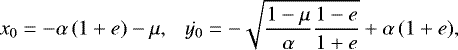 (5)
(5)
while in both cases we take  , thus following the approach used in Érdi et al. (2012).
The parameters e and α correspond to the eccentricity and semi-major axis of the test particle’s initial eccentric orbit, respectively. However, later on, the trajectory of the massless particle can be altered to some other type.
For the final state, regarding the type of motion of the test particle, we have three main categories: (i) trajectories that remain bounded and circulate around one or both main bodies, (ii) trajectories that lead to a collision with either the primary or the secondary, and (iii) trajectories that escape from the gravitational attraction of the binary system.
For the case of bounded trajectories, the motion of the test particle can be further classified as: (i) non-escaping regular, (ii) trapped sticky, and (ii) trapped chaotic, by using one of the available chaos indicators. In our study, we choose to apply the Smaller Alignment Index (SALI; Skokos 2001).
In the case of regular bounded motion, the test particle can circulate around one or both main bodies B1 and B2, while its orientation can be clockwise (retrograde) or counterclockwise (prograde or direct). The distinction between prograde and retrograde motion can be computationally achieved by simply obtaining the initial value of the angular momentum Lz0. At this point, we should clarify that the well-known equation Lz = xẏ − yẋ is valid only for trajectories that circulate around both or between the two main bodies, that is when the reference point regarding the direction of movement is the origin O. However, when the massless particle moves around one of the bodies B1 or B2, the equation of the angular momentum should be modified as  and
and  , respectively. In other words, the reference point, regarding the orientation of the movement, should be transferred from the origin O to the respective centers of the bodies B1 and B2.
In order to determine whether an ordered orbit circulates around one or both main bodies during the numerical integration, we computed the minimum (xmin) and the maximum (xmax) values of the coordinate x. Then, following the approach used in Nagler (2004, 2005), the regular trajectories can be further classified in the following eight sub-classes:
- 1.
Type 1a: if xmin < x1, xmax < x2 and Lz0 < 0 then the trajectory circulates around the primary B1, in a retrograde direction.
- 2.
Type 1b:if xmin < x1, xmax < x2 and Lz0 > 0 then the trajectory circulates around the primary B1, in a prograde direction.
- 3.
Type 2a: if xmin > x1, xmax > x2 and Lz0 < 0 then the trajectory circulates around the secondary B2, in a retrograde direction.
- 4.
Type 2b:if xmin > x1, xmax > x2 and Lz0 > 0 then the trajectory circulates around the secondary B2, in a prograde direction.
- 5.
Type 3a: if xmin < x1, xmax > x2 and Lz0 < 0 then the trajectory circulates around both bodies B1 and B2, in a retrograde direction.
- 6.
Type 3b: if xmin < x1, xmax > x2 and Lz0 > 0 then the trajectory circulates around both bodies B1 and B2, in a prograde direction.
- 7.
Type 4a: if xmin > x1, xmax < x2 and Lz0 < 0 then the trajectory circulates between both bodies B1 and B2, in a retrograde direction.
- 8.
Type 4b: if xmin > x1, xmax < x2 and Lz0 > 0 then the trajectory circulates between both bodies B1 and B2, in a prograde direction.
The schematics in Fig. 2 visualize the eight main possible types of regular orbits. Needless to say that the above sub-classes apply not only to periodic trajectories but also to quasi-periodic ones. Also, it is necessary to mention, that all the above-mentioned types of motion refer to the rotating system, thus the retrograde types are retrograde in the rotating system, but prograde in a fixed system, because the launch is in the direction of rotation.
A trajectory is considered to escape when the test particle moves far away from the system of the two bodies and therefore their gravitational attraction becomes infinitesimal. The threshold value for escape is set to  . On the other hand, the massless particle leads to a collision with either the primary B1 or the secondary B2, when r < 10−5.
The equations of motion (Eq. (1)) were numerically integrated by using a variable time step Bulirsch-Stoer integrator, while the corresponding routine was written in FORTRAN 77 (Press et al. 1992). The total time of the numerical integration was set to 104 time units (104∕2π revolutions), so as to ensure that all trajectories have enough time to unveil their true character. Throughout the computations, the conservation of the Jacobi constant C was sufficient enough, taking into account that the corresponding error was of the order of 10−14. The average required computation time, per color map, was varying between 10 h and 5 days, using a Quad-Core i7 4.0 GHz CPU (without using an MPI code), with 32 GB of RAM. The latest version 12.0 of MathematicaⓇ (Wolfram 2003) was utilized for the graphics of the article.
 |
Fig. 1 Planar configuration of the two main bodies B1 and B2, along with the massless particle m, which is launched either from its pericenter P, with velocityυp, or from its apocenter A, with velocityυa. In both cases, the vector of the initial velocity is perpendicular to the horizontal x-axis. O is the mass center of the bodies B1 and B2. |
 |
Fig. 2 Schematics illustrating the eight possible configurations of the bounded regular orbits. |
4 Orbit taxonomy in binary systems
The systemcontains three free parameters, that is the mass parameter μ, as well as the semi-major axis α along with the eccentricity e of the initial eccentric orbit of the test particle.
4.1 The (α, e) survey
We begin with maps on the (α, e)-plane for given values of μ. After retrieving from NASA Exoplanet Archive the updated data regarding the confirmed exoplanets, we choose those binary systems of parent star-exoplanet, in which the two main bodies move in circular orbits (so as to be able to use the circular version of the restricted three-body problem).
In Figs. 3a and b we present the basin diagrams on the (α, e)-plane, when μ = 0.0001. This value of the mass parameter corresponds to cases in which the exoplanet has a significantly smaller mass than the corresponding parent star. According to the so far obtained data, the exoplanets CoRoT-24 c and HD 103197 b, along with their parent stars, fit this particular value of the mass parameter. The test mass then takes the role of an additional planet or an exomoon around either CoRoT-24c or HD103197b, respectively. Part a of Fig. 3 corresponds to trajectories starting from the pericenter, while part b of the same figure contains trajectories launched from the apocenter of the initial eccentric orbit of the massless particle. In these diagrams, the black dashed line indicates the position where the apocentric distance is  , while the white dashed line marks the position where
  , that is when the pericenter of the massless particle reaches the orbit of the secondary (exoplanet).
We observe, that in both cases (launching from the pericenter or apocenter), when da < 1 the motion of the test particle is bounded. Specifically, the massless particle mainly moves in bounded regular trajectories around the primary (parent star). Moreover, when it is launched from its pericenter the motion is performed always in a prograde orientation (Type 1b), while when it is launched from its apocenter retrograde motion around the primary (Type 1a), is also possible. It should be noted, that for relatively high values of the eccentricity (e > 0.9) the chaotic and sticky motion dominates (see the upper left corners of the diagrams). The da > 1 part of the diagrams is divided into two main regions, where dp > 1 and dp < 1. The dp > 1 area is covered by a unified basin, corresponding to simple loop trajectories that circulate around both the parent star and the exoplanet, while the dp < 1 area contains numerous islands of resonant orbits that also circulate around both main bodies of the system. All types of motion around B1 and B2 are retrograde (Type 3a), while there is no numerical indication of prograde motion around them (Type 3b). Inside the dp < 1 region one can identify some small islands of starting conditions, corresponding to Type 2a motion, that is retrograde motion around the exoplanet, while prograde motion around the secondary seems to be absent.
Around the line dp = 1 we see a mixture of starting conditions that correspond either to chaotic/sticky motion or to collision with the exoplanet. It is interesting to note that for such small values of the mass parameter, escaping trajectories, as well as trajectories leading to a collision with the parent star (primary), are extremely limited. Indeed, our computations suggest that both types of motion are possible, however, the corresponding starting conditions appear only as isolated points, scattered in the dp < 1 area, without forming basins of escape or collision.
It should be noted, that in all studied cases, we encountered a small portion of sticky orbits. However, the corresponding starting conditions appear only as lonely points (not forming regions) and they are always deeply embedded inside the chaotic yellow regions of the color-coded maps. Therefore they are not quite visible.
In Fig. 4 we provide the distribution of the values of the Jacobi constant, for the starting conditions of part a of Fig. 3. We see, that for relatively low values of the semi-major axis (α < 0.4) we measured the highest values of C, while the lowest values of the Jacobi constant correspond to starting conditions with e > 0.9. It is interesting to note how the values of C spike when dp = 1. This happens because when dp = α(1 − e) = 1 the second term in the effective potential Φ(x, y) becomes singular. Exactly along the curve dp = 1 the initial conditions lead to an immediate collision with the secondary and therefore the numerical integration is not possible for them. This curve acts, in a way, as an additional forbidden region. However, initial conditions outside this line (from both sides) can be numerically integrated and the respective values of the Jacobi constant are relatively high, since we are in the near vicinity of a “forbidden region”.
According to the data from NASA Exoplanet Archive, for the majority of the exoplanetary systems, that can be modeled by the restricted three-body problem, the value of the mass parameter is about μ =0.001. In Table 1 we provide the details of 33 exoplanetary systems with compatible values of μ. We note that in most of the cases presented in Table 1 the exoplanet is the sole exoplanet in the respective exosolar system.
In Figs. 5a and b we depict the basin diagrams on the (α, e)-plane, for μ =0.001. For the regions withda < 1 the orbital structure is quite similar to that we have seen earlier in Fig. 3. Moreover, we can nowclearly see the stability islands of the resonant periodic orbits, located in the dp < 1 region. Figure 6 shows ten characteristic resonant periodic orbits, with starting conditions from part a of Fig. 5. One can see, that initially, the trajectory circulates around the exoplanet (see part a), while with increasing value of the semi-major axis, the trajectory evolves around both bodies (star and exoplanet), while at the same time it becomes much more complicated (in other words its multiplicity increases). The positions of the ten periodic solutions on the (α, e) plane are shown in part a of Fig. 5, using black five-pointed stars.
When the trajectories are launched from the pericenter (see part a of Fig. 5) around the line dp = 1 we can see the stability islands corresponding to both retrograde (Type 2a) and prograde (Type 2b) motion around the exoplanet. The first type of stability islands is located just above the curve dp = 1, while the second type of stability islands can be seen just below the same curve. In addition, in part b of Fig. 5 we observe that the two regions dp < 1 and dp > 1 are somehow connected, through the continuation of stability islands, corresponding to Type 3a motion. When μ =0.001, the presence of escaping trajectories, in the dp < 1 region, is stronger, while also collision orbits to the primary are present, mainly for e > 0.8.
The next value of the mass parameter under consideration is μ =0.01, while characteristic examples of exoplanets, with compatible values of μ, are the NN Ser (AB) c and RR Cae b. Figs. 7a and b displays the basin structure on the (α, e)-plane, for μ = 0.01. The most prominent aspects of the orbital dynamics of the test particle are the following: (i) the stability islands of the resonant orbits in the dp < 1 area are reduced, especially in the case where the test particle is launched from its apocenter, (ii) the area of the stability islands, corresponding to Type 2a and 2b trajectories around the exoplanet (which exist around the curve dp = 1) increases, (iii) retrograde regular motion (Type 1a) around the primary is possible only in the case of a launch from the apocenter, (iv) regular motion (both prograde and retrograde) around the exoplanet is possible only when the masslessparticle is launched from its pericenter, and (v) basins composed of starting conditions leading to a collision with the exoplanet mainly exist when the test particle is launched from its pericenter, while in the case that it is launched from its apocenter the same type of collision trajectories form significantly smaller basins of collision.
From the catalog of the exoplanets, the highest possible value of the mass parameter is μ =0.1875 and it corresponds to the exoplanetary system 2M 2206-20. The respective character of motion of the test particle on the (α, e)-plane is given in Figs. 8a and b. Here, it is evident that the basin structure has many differences, with respect to the previously studied cases. In the case where the test particle is launched from its pericenter (see part a), first of all, one can observe the complete absence of trajectories (simple or of higher resonance) that revolve around both main bodies (Type 3a). In fact, the dp > 1 part of the (α, e)-plane is now covered by a complicated mixture of escaping and collision trajectories. In the dp < 1 part of the same plane, there is still one main stability island of retrograde trajectories around the exoplanet, but there is no evidence of prograde motion around the secondary. Furthermore, it should be noted that for this value of the mass parameter, it is the first time that starting conditions that lead to a collision with the primary (star) form substantial basins of collision.
In the case that the massless particle is launched from its apocenter (see part b of Fig. 8) retrograde regular motion around both bodies (Type 3a) dominates the (α, e)-plane. Specifically, the corresponding stability island crosses the curve dp = 1 and covers both regions with dp < 1 and dp > 1. Another interesting aspect is the fact that the retrograde motion around the primary (Type 1a) is extremely confined, while a small stability island is present in the da < 1 area and for relatively high values of the eccentricity (e > 0.8). Moreover, one can see, that in this case, the basin boundaries of the stability island of Type 3a motion are more smooth. In particular, in all previous cases we have seen that in the vicinity of the basin boundaries of the stability islands of Type 3a motion, there was a considerable amount of starting conditions corresponding to trapped chaotic motion. However, in this case, it is seen that the rate of chaotic motion is much lower.
Figures 9a and b shows the character of motion of the massless particle, for μ = 0.4. Of course, such high values of the mass parameter are not possible in a binary system of star-exoplanet, but they are possible in other types of exoplanetary systems, such as exoplanet-exoplanet or even exoplanet-exomoon (see e.g., Teachey & Kipping 2018). In such cases, the role of the test particle could be played by an asteroid/comet or a space probe. With respect to the previous case, the orbital content on the (α, e)-plane has several major differences. In the case of launching the test particle from its pericenter (see part a of Fig. 9) regular bounded motion around the exoplanet is no longer dynamically possible, while the area of the collision basin to secondary has been increased. Moreover, the area of the basin corresponding to regular prograde motion around the primary has been further confined. Part b of Fig. 9 shows the final states of the test particle when it has been launched from the apocenter. Now escaping motion is the dominant type of motion (especially in the dp > 1 region), while at the same time, the stability island which contains the starting conditions of simple retrograde trajectories around both bodies (Type 3a) has been almost completely transferred to the dp < 1 region of the (α, e)-plane.
The pericentric velocity of the test particle decreases when the value of α increases. Thus, for α < 1 the test particle is launched with larger velocity, than the circular velocity of the secondary. Therefore, in the rotatingsystem, the orbit of the test particle is direct (meaning the direction of rotation). However, for α >1 the test particle is launched with smaller velocity than the circular velocity of the secondary and thus the test particle moves slower than the primaries. Viewing thisfrom the rotating system, the test particle moves backward, in a retrograde direction. The above analysis explains why for α <1 we see a strong presence of Type 1b motion and also why for α > 1 the dominant type of regular motion is Type 3a. Moreover, to obtain Type 3b trajectories, the test particle must be started perpendicularly to the x-axis but in the opposite direction of the rotation of the primary.
 |
Fig. 3 Color diagrams showing the basins on the (α, e)-plane, for μ = 0.0001, when the test particle is launched from its (a) pericenter, and (b) apocenter. The black dashed line marks the position where the apocenter distance is α(1 + e) = 1, while the white dashed line indicates the position where the pericenter distance is α(1 − e) = 1. |
 |
Fig. 4 Distribution of the values of the Jacobi constant, for the starting conditions, shown in part a of Fig. 3. The red curve corresponds to dp = 1. |
Data of confirmed exoplanets: mass of the exoplanet mp (in Jupiter masses MJ), mass of the parent star ms (in solar masses M⊙), and the corresponding value of the mass parameter μ.
 |
Fig. 5 Color diagrams showing the basins on the (α, e)-plane, for μ = 0.001, when the test particle is launched from its (a) pericenter and (b) apocenter. The black dashed line marks the position where the apocenter distance is α(1 + e) = 1, while the white dashed line indicates the position where the pericenter distance is α(1 − e) = 1. The black five-pointed stars indicate the position of the periodic orbits of Fig. 6. |
 |
Fig. 6 Sample characteristic resonant periodic orbits, when μ = 0.001, with starting conditions from part a of Fig. 5. The red dots pinpoint the locations of the two bodies (star and exoplanet). |
 |
Fig. 7 Color diagrams showing the basins on the (α, e)-plane, for μ = 0.01, when the test particle is launched from its (a) pericenter and (b) from its apocenter. The black dashed line marks the position where the apocenter distance is α(1 + e) = 1, while the white dashed line indicates the position where the pericenter distance is α(1 − e) = 1. |
 |
Fig. 8 Color diagrams showing the basins on the (α, e)-plane, for μ = 0.1875, when the test particle is launched from its (a) pericenter and (b) apocenter. The black dashed line marks the position where the apocenter distance is α(1 + e) = 1, while the white dashed line indicates the position where the pericenter distance is α(1 − e) = 1. |
 |
Fig. 9 Color diagrams showing the basins on the (α, e)-plane, for μ = 0.4, when the test particle is launched from its (a) pericenter and (b) apocenter. The black dashed line marks the position where the apocenter distance is α(1 + e) = 1, while the white dashed line indicates the position where the pericenter distance is α(1 − e) = 1. |
4.2 The (α, μ) survey
So far, we studied the character of motion with starting conditions on the (α, e)-plane, for specific values of the mass parameter μ. Now, we will provide results on the (α, μ)-plane, for specific values of the eccentricity e. Figures 10a–f shows the orbital structure of the (α, μ)-plane when the test particle is launched from its pericenter. In this type of 2D color map, we can clearly distinguish how the mass parameter influences the motion of the test particle. One can observe the following phenomena: (i) retrograde motion around both main bodies (Type 3a) exists only for μ <0.1 and also when e < 0.6, (ii) prograde motion around the primary is almost always possible, for relatively low values of the semi-major axis (α < 0.5). However, for extremely high values of the eccentricity (e.g., when e = 0.95) the regular motion turns to chaotic, (iii) prograde and retrograde motion around the exoplanet is possible mainly for μ < 0.2, while the corresponding stability islands are situated around the line dp = 1, as it can be seen on parts c and d of Fig. 10, (iv) around both sides of the line dp = 1 we see the presence of a basin composed of starting conditions leading to a collision with the exoplanet. With increasing value of the eccentricity the size of this basin grows, while at the same time its location moves to higher values of the semi-major axis, and (v) the remaining area of the (α, μ)-plane is covered by a mixture of starting conditions that form basins of escape and collision with highly complicated shapes.
In Figs. 11a–f we present the basin diagrams on the (α, μ)-plane when the test particle is launched from its apocenter. In this case, we see that the changes in the orbital structure are milder, with respect to what we have seen in the previous case when the test particle is launched from its pericenter. As the value of the eccentricity increases, the most important change concerns the stability island of the Type 3a trajectories. Specifically, the stability island moves on higher values of μ, with an increasing value of e. Moreover, the same stability island divides the (α, μ)-plane into two regions: (i) the region above the island, which is completely dominated by escaping trajectories and (ii) the region below the stability islands, which contains a rich mixture of starting conditions, corresponding to both escaping and collision trajectories.
One should expect that the dynamics on the (α, μ)-plane would be the same when e = 0. However, looking at parts a of Figs. 10 and 11 it is evident that this is not true. Indeed, for e = 0 there is no pericenter and apocenter, but according to the Eqs. (4) and (5), the test particle is launched from two different initial positions on the x-axis with respect to the primaries, hence the observed differences in its orbital nature.
 |
Fig. 10 Color diagrams showing the basins on the (α, μ)-plane, when the test particle is launched from its pericenter, for (a): e = 0, (b): e = 0.2, (c): e = 0.4, (d): e = 0.6, (e): e = 0.8, (f): e = 0.95. The black dashed line marks the position where the apocenter distance is α(1 + e) = 1, while the white dashed line indicates the position where the pericenter distance is α(1 − e) = 1. |
4.3 The (μ,e) survey
The last type of map under consideration lies on the (μ, e)-plane. In Figs. 12a–i we present the nature of the motion of the test particle when it is launched from its pericenter, for α ≤1. In part a, where α =0.2, it is seen, that almost all the map is covered by starting conditions that correspond to prograde orbits around the primary. Only at extremely high values of the eccentricity (e > 0.9) trapped chaotic motion appears, along with collision trajectories. As the value of the semi-major axis increases (see parts b and c) the portion of the prograde Type 1b trajectories is reduced, while at the same time collision and escape type of motion emerge, from the right-hand side of the diagrams. When α =0.5 (part d) and α =0.6 (part e) the structure of the (μ, e)-plane is very complicated, with a fractal-like geometry (see e.g., Aguirre et al. 2001, 2009). More specifically, the unified stability island of Type 1b motion splits into several smaller bounded basins, while the escape and collision basins form spiral structures. For α ≥0.7 Type 1b motion is hardly visible and it is present only for low values of the mass parameter. Moreover, a basin, corresponding to collision trajectories to the secondary, establishes (at the lower right part of the diagrams) and its size grows with an increasing value of α. For α ≥0.9 at the upper left corner of the (μ, e)-plane we see the presence of new stability islands corresponding to retrograde motion around the secondary (Type 2a), while for higher values of the eccentricity the type of the trajectories changes to Type 3a, thus revolving around both main bodies.
The orbital properties of the massless particle, when it is launched from its apocenter, are given in Figs. 13a–i. For relatively low values of the semi-major axis (see parts a–c) the structure of the (μ, e)-plane is fairly close to what we have seen earlier in Fig. 12. The only major difference is the fact that now retrograde trajectories around the primary (Type 1a) are also possible, for high values of the eccentricity. Again, the most strange and complicated basin structures of collision trajectories occur when 0.5 ≤ α ≤ 0.7. For higher values of the semi-major axis Type 1b motion disappears, while the strength of the collision basins weakens. In addition, at the right-hand side of the diagrams, we see the appearance of new stability islands, formed of starting conditions corresponding to retrograde trajectories around both main bodies (Type 3a). Also, it should be noted that when the semi-major axis of the initial eccentric orbit of the test particle tends to 1, Type 1a motion is also possible, for relatively low and high values of μ and e, respectively.
In Figs. 14a–d we display additional color maps on the (μ, e)-plane, for values of the semi-major axis larger than 1, when the test particle is launched from its pericenter. We see that: (i) a basin, corresponding to trajectories leading to a collision with the secondary, exists around the region, where the pericenter distance is equal to 1. The area of this collision basin is reduced, while its relative position moves to higher values of e, with increasing value of the semi-major axis, (ii) at the lower-left corner of the (μ, e)-plane a stability island emerges, corresponding to trajectories moving around both main bodies, in a retrograde orientation. The area of this bounded basin increases, as we proceed to higher values of α, and (iii) when α > 1 both types of ordered motion around the secondary (that is, Types 2a and 2b) are possible, with respective basins situated around the line dp = 1.
In the same vein, Figs. 15a–d shows the color maps on the (μ, e)-plane, for α > 1, when the test particle is launched from its apocenter. In this case, the orbital structure of the basin diagram is less interesting, with respect to those of Fig. 14. It is seen, that stability island, corresponding to Type 3a motion, covers a large portion of the (μ, e)-plane, while its area seems to reduced, with increasing value of the semi-major axis. At the boundaries of this stability island, we have the presence of trapped chaotic motion, which is an expected phenomenon. The region below the stability islands of the Type 3a motion is completely smooth and it is dominated by a unified basin of escape. On the other hand, the region above the same stability island is covered by a noisy mixture of escaping and collision (to both main bodies) starting conditions.
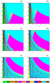 |
Fig. 11 Color diagrams showing the basins on the (α, μ)-plane, when the test particle is launched from its apocenter, for (a): e = 0, (b): e = 0.2, (c): e = 0.4, (d): e = 0.6, (e): e = 0.8, (f): e = 0.95. The black dashed line marks the position where the apocenter distance is α(1 + e) = 1, while the white dashed line indicates the position where the pericenter distance is α(1 − e) = 1. |
 |
Fig. 12 Color diagrams showing the basins on the (μ, e)-plane, when the test particle is launched from its pericenter, for (a): α = 0.2, (b): α = 0.3, (c): α = 0.4, (d): α = 0.5, (e): α = 0.6, (f): α = 0.7, (g): α = 0.8, (h): α = 0.9, (i): α = 1.0. The black dashed line marks the position where the apocenter distance is α(1 + e) = 1. |
 |
Fig. 13 Color diagrams showing the basins on the (μ, e)-plane, when the test particle is launched from its apocenter, for (a): α = 0.2, (b): α = 0.3, (c): α = 0.4, (d): α = 0.5, (e): α = 0.6, (f): α = 0.7, (g): α = 0.8, (h): α = 0.9, (i): α = 1.0. The black dashed line marks the position where the apocenter distance is α(1 + e) = 1. |
 |
Fig. 14 Color diagrams showing the basins on the (μ, e)-plane, when the test particle is launched from its pericenter, for (a): α = 2, (b): α = 3, (c): α = 4, (d): α = 5. The while the white dashed line indicates the position where the pericenter distance is α(1 − e) = 1. |
 |
Fig. 15 Color diagrams showing the basins on the (μ, e)-plane, when the test particle is launched from its apocenter, for (a): α = 2, (b): α = 3, (c): α = 4, (d): α = 5. The white dashed line indicates the position where the pericenter distance is α(1 − e) = 1. |
5 Conclusions
In this article, we combined the theory of the restricted three-body problem along with the numerical technique of grid classification, in order to predict the nature of the trajectories of a test particle moving in a binary exoplanetary system. Specifically, the binary system could be composed of a parent star along with an exoplanet, two exoplanets, or an exoplanet with an exomoon, while the third body (test particle) can be an asteroid/comet, a space probe, or even a small exomoon in the case where the primary is a star. Using the grid classification method, we managed to obtain the character of the motion of the massless particle and classify the corresponding starting conditions in three classes: (i) bounded, (ii) escaping and (iii) collision. In the case of regular bounded motion, additional criteria were used for deriving their geometry (revolving around one or both main bodies) and orientation (prograde or retrograde). For the test particle, we considered two scenarios, regarding its initial position, that is launched either from its pericenter or apocenter. The basin diagrams on the several types of color-coded 2D maps helped us to visualize the final states of the test particle.
Specifically, our analysis suggests that the influence of the mass parameter μ, along with the semi-major axis α and the eccentricity e of the initialeccentric trajectory of the test particle is as follows:
-
Retrograde regular motion around the primary (Type 1a) exists for α < 1 and onlywhen the test particle is launched from its apocenter.
-
Prograde regular motion around the primary (Type 1b) exists for α < 1 for both pericentric and apocentric launching of the test particle.
-
Bounded regular motion around the secondary (Types 2a and 2b) exists only when the massless particle starts from its pericenter. Moreover, Type 2a is present for dp < 1 and Type 2b for dp > 1.
-
Simple retrograde trajectories around both bodies (Type 3a) were found and are present for dp > 1, for both pericentric and apocentric launching.
-
Resonant retrograde trajectories around both bodies (Type 3a) exist for μ < 0.1, α > 1, dp < 1, while they are possible only when the test particle is launched from its pericenter.
-
Collision trajectories to secondary are mainly present around dp = 1. Furthermore, the area of the respective type of basin grows, with an increasing value of μ, while it reduces as the value of the semi-major axis α increases.
-
Escaping motion seems to completely dominate for relatively high values of the mass parameter (μ > 0.3) and the semi-major axis (α > 3), in the case of apocentric launching.
-
For relatively high values of the eccentricity (e > 0.9) the regular types of motion 1a and 1b turn to chaotic.
-
Our computations suggest, that prograde motion around both main bodies (Type 3b), along with motion (prograde and retrograde) between them (Types 4a and 4b) is not possible, at least for the used type of initial conditions of the test particle.
-
For 0.4 < α < 0.6 the orbital properties of the test particle are very complicated, thus leading to highly interesting basin diagrams with a fractal-like geometry.
Additionally, it should be stated, that in exoplanetary systems that contain only one exoplanet (see Table 1) further smaller exoplanets could exist. The positions of these hidden exoplanets should be the stable regions of the systems, as they have been presented in the basin color-coded diagrams.
In closing, we would like to emphasize that the present orbit classification in exoplanetary systems is novel since there are no previous studies containing such a systematic and detailed analysis of the final states of the trajectories of the test particle. On this basis, we claim that our contribution contains new and interesting information which advances our existing knowledge regarding the orbital dynamics around exoplanets.
Acknowledgements
This project was funded by the Deanship of Scientific Research (DSR) at King Abdulaziz University, Jeddah, Saudi Arabia, under grant number (KEP-42-130-38). The authors, therefore, acknowledge with thanks DSR for technical and financial support. The first author (E.E.Z.) thanks Dr. Christof Jung for illuminating discussions, during the investigation. The authorswould also like to express their warmest thanks to the anonymous referee for the careful reading of the manuscript as well as for all the apt suggestions and comments which allowed us to improve both the quality and the clarity of the paper.
References
- Aguirre, J., Vallejo, J. C., & Sanjuán, M. A. F. 2001, Phys. Rev. E, 64, 066208 [NASA ADS] [CrossRef] [Google Scholar]
- Aguirre, J., Viana, R. L., & Sanjuán, M. A. F. 2009, Rev. Mod. Phys., 81, 333 [NASA ADS] [CrossRef] [Google Scholar]
- Antoniadou, K. I. 2016, Eur. Phys. J. Spec. Top., 225, 1001 [NASA ADS] [CrossRef] [Google Scholar]
- Antoniadou, K. I., & Voyatzis, G. 2014, Astrophys. Space Sci., 349, 657 [NASA ADS] [CrossRef] [Google Scholar]
- Antoniadou, K. I., & Voyatzis, G. 2016, MNRAS, 461, 3822 [NASA ADS] [CrossRef] [Google Scholar]
- Campanella, G. 2011, MNRAS, 418, 1028 [NASA ADS] [CrossRef] [Google Scholar]
- Campanella, G., Nelson, R. P., & Agnor, C. B. 2013, MNRAS, 433, 3190 [NASA ADS] [CrossRef] [Google Scholar]
- Correia, A. C. M., Couetdic, J., Laskar, J., et al. 2010, A&A 511, A21 [NASA ADS] [CrossRef] [EDP Sciences] [Google Scholar]
- Couetdic, J., Laskar, J., Correia, A. C. M., Mayor, M., & Udry, S. 2010, A&A, 519, A10 [NASA ADS] [CrossRef] [EDP Sciences] [Google Scholar]
- Érdi, B. 1977, Celest. Mech., 15, 367383 [Google Scholar]
- Érdi, B., & Sándor, Zs. 2005 Celest. Mech. Dyn. Astron., 92, 113 [NASA ADS] [CrossRef] [Google Scholar]
- Érdi, B., Rajnai, R., Sándor, Z., & Forgács-Dajka, E. 2012, Celest. Mech. Dyn. Astron., 113, 95 [NASA ADS] [CrossRef] [Google Scholar]
- Ferraz-Mello, S., Michtchenko, T. A., & Beaugé, C. 2006, Chaotic Worlds: from Order to Disorder in Gravitational N-Body Dynamical Systems, eds. B. A. Steves, A. J. Maciejewski, & M. Hendry (Berlin: Springer), 255 [Google Scholar]
- Funk, B., Schwarz, R., Süli, A., & Érdi, B. 2012, MNRAS, 423, 3074 [NASA ADS] [CrossRef] [Google Scholar]
- Goździewski, K., Konacki, M., & Maciejewski, A. J. 2006, ApJ, 645, 688 [NASA ADS] [CrossRef] [Google Scholar]
- Hadjidemetriou, J. D. 2006, Celest. Mech. Dyn. Astron., 95, 225 [NASA ADS] [CrossRef] [Google Scholar]
- Henrard, J., & Libert, A.-S. 2008, Celest. Mech. Dyn. Astron., 102, 177 [NASA ADS] [CrossRef] [Google Scholar]
- Hippke, M., & Angerhausen, D. 2015, ApJ, 811, 5 [NASA ADS] [CrossRef] [Google Scholar]
- Laskar, L., & Correia, A. C. M. 2009, A&A, 496, L5 [NASA ADS] [CrossRef] [EDP Sciences] [Google Scholar]
- Laughlin, G., & Chambers, J. E. 2002, AJ, 124, 592 [NASA ADS] [CrossRef] [Google Scholar]
- Lee, M. H. 2004, ApJ, 611, 517 [NASA ADS] [CrossRef] [Google Scholar]
- Leleu, A., Robutel, P., Correia, A. C. M., & Lillo-Box, J. 2017, A&A, 599, A4 [Google Scholar]
- Lovis, C., Ségransan, D., Mayor, M., et al. 2011, A&A, 528, A112 [NASA ADS] [CrossRef] [EDP Sciences] [Google Scholar]
- Michtchenko, T. A., Beaugé, C., & Ferraz-Mello, S. 2006, Celest. Mech. Dyn. Astron., 94, 411 [NASA ADS] [CrossRef] [MathSciNet] [Google Scholar]
- Mikkola, S., Innanen, K., Wiegert, P., Connors, M., & Brasser, R. 2006, MNRAS, 369, 15 [NASA ADS] [CrossRef] [Google Scholar]
- Morais, M. H. M., & Namouni, F. 2013, Celest. Mech. Dyn. Astron., 117, 405 [NASA ADS] [CrossRef] [Google Scholar]
- Murray, C., & Dermott, S. 1999, Solar System Dynamics (Cambridge: Cambridge Univesristy Press) [Google Scholar]
- Nagler, J. 2004, Phys. Rev. E, 69, 066218 [NASA ADS] [CrossRef] [EDP Sciences] [Google Scholar]
- Nagler, J. 2005, Phys. Rev. E, 71, 026227 [NASA ADS] [CrossRef] [Google Scholar]
- Namouni, F. 1999, Icarus, 137, 293 [NASA ADS] [CrossRef] [Google Scholar]
- Pousse, A., Robutel, P., & Vienne, A. 2017, Celest. Mech. Dyn. Astron., 128, 383 [NASA ADS] [CrossRef] [Google Scholar]
- Press, H. P., Teukolsky, S. A, Vetterling, W. T., & Flannery, B. P. 1992, Numerical Recipes in FORTRAN, 2nd edn., (Cambridge: Cambridge Univ. Press), 77 [Google Scholar]
- Rein, H., Papaloizou, J. C. B., & Kley, W. 2010, A&A, 510, A4 [NASA ADS] [CrossRef] [EDP Sciences] [Google Scholar]
- Robutel, P., & Pousse, A. 2013, Celest. Mech. Dyn. Astron., 117, 17 [NASA ADS] [CrossRef] [Google Scholar]
- Schwarz, R., Bazso, A., Érdi, B., & Funk, B. 2012, MNRAS, 427, 397 [NASA ADS] [CrossRef] [Google Scholar]
- Sidorenko, V., Artemiev, A., Neishtadt, A., & Zelenyi, L. 2014, Celest. Mech. Dyn. Astron., 120, 131 [NASA ADS] [CrossRef] [Google Scholar]
- Skokos, C. 2001, J. Phys. A Math. Gen, 34, 10029 [NASA ADS] [CrossRef] [MathSciNet] [Google Scholar]
- Teachey, A., & Kipping, D. M. 2018, Sci. Adv., 4, 1784 [NASA ADS] [CrossRef] [Google Scholar]
- Voyatzis, G. 2008, ApJ, 675, 802 [NASA ADS] [CrossRef] [Google Scholar]
- Wolfram, S. 2003, The Mathematica Book Champaign: Wolfram Media [Google Scholar]
All Tables
Data of confirmed exoplanets: mass of the exoplanet mp (in Jupiter masses MJ), mass of the parent star ms (in solar masses M⊙), and the corresponding value of the mass parameter μ.
All Figures
|
Fig. 1 Planar configuration of the two main bodies B1 and B2, along with the massless particle m, which is launched either from its pericenter P, with velocityυp, or from its apocenter A, with velocityυa. In both cases, the vector of the initial velocity is perpendicular to the horizontal x-axis. O is the mass center of the bodies B1 and B2. |
| In the text | |
|
Fig. 2 Schematics illustrating the eight possible configurations of the bounded regular orbits. |
| In the text | |
|
Fig. 3 Color diagrams showing the basins on the (α, e)-plane, for μ = 0.0001, when the test particle is launched from its (a) pericenter, and (b) apocenter. The black dashed line marks the position where the apocenter distance is α(1 + e) = 1, while the white dashed line indicates the position where the pericenter distance is α(1 − e) = 1. |
| In the text | |
|
Fig. 4 Distribution of the values of the Jacobi constant, for the starting conditions, shown in part a of Fig. 3. The red curve corresponds to dp = 1. |
| In the text | |
|
Fig. 5 Color diagrams showing the basins on the (α, e)-plane, for μ = 0.001, when the test particle is launched from its (a) pericenter and (b) apocenter. The black dashed line marks the position where the apocenter distance is α(1 + e) = 1, while the white dashed line indicates the position where the pericenter distance is α(1 − e) = 1. The black five-pointed stars indicate the position of the periodic orbits of Fig. 6. |
| In the text | |
|
Fig. 6 Sample characteristic resonant periodic orbits, when μ = 0.001, with starting conditions from part a of Fig. 5. The red dots pinpoint the locations of the two bodies (star and exoplanet). |
| In the text | |
|
Fig. 7 Color diagrams showing the basins on the (α, e)-plane, for μ = 0.01, when the test particle is launched from its (a) pericenter and (b) from its apocenter. The black dashed line marks the position where the apocenter distance is α(1 + e) = 1, while the white dashed line indicates the position where the pericenter distance is α(1 − e) = 1. |
| In the text | |
|
Fig. 8 Color diagrams showing the basins on the (α, e)-plane, for μ = 0.1875, when the test particle is launched from its (a) pericenter and (b) apocenter. The black dashed line marks the position where the apocenter distance is α(1 + e) = 1, while the white dashed line indicates the position where the pericenter distance is α(1 − e) = 1. |
| In the text | |
|
Fig. 9 Color diagrams showing the basins on the (α, e)-plane, for μ = 0.4, when the test particle is launched from its (a) pericenter and (b) apocenter. The black dashed line marks the position where the apocenter distance is α(1 + e) = 1, while the white dashed line indicates the position where the pericenter distance is α(1 − e) = 1. |
| In the text | |
|
Fig. 10 Color diagrams showing the basins on the (α, μ)-plane, when the test particle is launched from its pericenter, for (a): e = 0, (b): e = 0.2, (c): e = 0.4, (d): e = 0.6, (e): e = 0.8, (f): e = 0.95. The black dashed line marks the position where the apocenter distance is α(1 + e) = 1, while the white dashed line indicates the position where the pericenter distance is α(1 − e) = 1. |
| In the text | |
|
Fig. 11 Color diagrams showing the basins on the (α, μ)-plane, when the test particle is launched from its apocenter, for (a): e = 0, (b): e = 0.2, (c): e = 0.4, (d): e = 0.6, (e): e = 0.8, (f): e = 0.95. The black dashed line marks the position where the apocenter distance is α(1 + e) = 1, while the white dashed line indicates the position where the pericenter distance is α(1 − e) = 1. |
| In the text | |
|
Fig. 12 Color diagrams showing the basins on the (μ, e)-plane, when the test particle is launched from its pericenter, for (a): α = 0.2, (b): α = 0.3, (c): α = 0.4, (d): α = 0.5, (e): α = 0.6, (f): α = 0.7, (g): α = 0.8, (h): α = 0.9, (i): α = 1.0. The black dashed line marks the position where the apocenter distance is α(1 + e) = 1. |
| In the text | |
|
Fig. 13 Color diagrams showing the basins on the (μ, e)-plane, when the test particle is launched from its apocenter, for (a): α = 0.2, (b): α = 0.3, (c): α = 0.4, (d): α = 0.5, (e): α = 0.6, (f): α = 0.7, (g): α = 0.8, (h): α = 0.9, (i): α = 1.0. The black dashed line marks the position where the apocenter distance is α(1 + e) = 1. |
| In the text | |
|
Fig. 14 Color diagrams showing the basins on the (μ, e)-plane, when the test particle is launched from its pericenter, for (a): α = 2, (b): α = 3, (c): α = 4, (d): α = 5. The while the white dashed line indicates the position where the pericenter distance is α(1 − e) = 1. |
| In the text | |
|
Fig. 15 Color diagrams showing the basins on the (μ, e)-plane, when the test particle is launched from its apocenter, for (a): α = 2, (b): α = 3, (c): α = 4, (d): α = 5. The white dashed line indicates the position where the pericenter distance is α(1 − e) = 1. |
| In the text | |
Current usage metrics show cumulative count of Article Views (full-text article views including HTML views, PDF and ePub downloads, according to the available data) and Abstracts Views on Vision4Press platform.
Data correspond to usage on the plateform after 2015. The current usage metrics is available 48-96 hours after online publication and is updated daily on week days.
Initial download of the metrics may take a while.