| Issue |
A&A
Volume 634, February 2020
|
|
|---|---|---|
| Article Number | A70 | |
| Number of page(s) | 21 | |
| Section | Astronomical instrumentation | |
| DOI | https://doi.org/10.1051/0004-6361/201936379 | |
| Published online | 11 February 2020 | |
Tips and tricks in linear imaging polarimetry of extended sources with FORS2 at the VLT⋆
1
CENTRA-Centro de Astrofísica e Gravitação and Departamento de Física, Instituto Superior Técnico, Universidade de Lisboa, Avenida Rovisco Pais, 1049-001 Lisboa, Portugal
e-mail: This email address is being protected from spambots. You need JavaScript enabled to view it.
2
ESO – European Southern Observatory, Karl-Schwarzschild-Str. 2, 85748 Garching b. München, Germany
3
European Southern Observatory, Alonso de Córdova 3107, Casilla 19, Santiago, Chile
4
Physics Division, Lawrence Berkeley National Laboratory, 1 Cyclotron Road, Berkeley, CA 94720, USA
5
Department of Physics, University of Warwick, Gibbet Hill Road, Coventry CV4 7AL, UK
6
Department of Physics and Astronomy, University of Leicester, University Road, Leicester LE1 7RH, UK
Received:
24
July
2019
Accepted:
18
December
2019
Abstract
Context. Polarimetry is a very powerful tool for uncovering various properties of astronomical objects that otherwise remain hidden in standard imaging or spectroscopic observations. While common observations only measure the intensity of light, polarimetric measurements allow us to distinguish and measure the two perpendicular components of the electric field associated with the incoming light. By using polarimetry it is possible to unveil asymmetries in supernova explosions, properties of intervening dust, characteristics of atmosphere of planets, among others. However, the reliable measurement of the low polarization signal from astronomical sources requires a good control of spurious instrumental polarization induced by the various components of the optical system and the detector.
Aims. We perform a detailed multi-wavelength calibration study of the FORS2 instrument at the VLT operating in imaging polarimetric mode to characterize the spatial instrumental polarization that may affect the study of extended sources.
Methods. We used imaging polarimetry of high signal-to-noise ratio blank field BVRI observations during the full moon, when the polarization is expected to be constant across the field of view and deviations originate from the instrument, and a crowded star cluster in broad-band RI and narrow-band Hα filters, where the individual polarization values of each star across the field can be measured.
Results. We find an instrumental polarization pattern that increases radially outwards from the optical axis of the instrument reaching up to 1.4% at the edges, depending on the filter. Our results are closely approximated by an elliptical paraboloid down to less than ∼0.05% accuracy, and ∼0.02% when using non-analytic fits. We present 2D maps to correct for this spurious instrumental polarization. We also give several tips and tricks for analyzing polarimetric measurements of extended sources.
Conclusions. FORS2 is a powerful instrument that allows the linear polarimetry of extended sources to be mapped. We present and discuss a methodology that can be used to measure the polarization of such sources, and to correct for the spatial polarization induced in the optical system. This methodology could be applied to polarimetric measurements using other dual-beam polarimeters.
Key words: instrumentation: polarimeters / techniques: polarimetric
Based on observations made with FORS2 at the VLT, ESO under programs 60.A-9800(C) and 0101.D-0142(A).
© ESO 2020
1. Introduction
“Our scientific work in physics consists in asking questions about nature in the language that we possess and trying to get an answer from experiment by the means that are at our disposal.” Heisenberg (1958).
The polarization of light can carry relevant information about the emission and transmission processes occurring in astronomical objects, their surroundings, and the material in the line of sight. Polarization is found in the light from nearby stars to stellar clusters, up to high-redshift galaxies, and can be produced through emission mechanisms like synchrotron emission or indirectly through absorption or scattering in the interstellar medium (see Hough 2006 for a review). From asymmetries in supernova explosions (e.g., Reilly et al. 2017) to large-scale magnetic fields in galaxies (e.g., Momose et al. 2001), polarimetry provides an extremely powerful tool for unveiling their physical properties, otherwise hidden in common photometric or spectroscopic observations.
Despite the importance of polarimetric observations, carrying out polarization measurements can be a challenging task. The measurement of the low degree of polarization of most astronomical sources (on the order of few percent or even less than a percent) requires high signal-to-noise ratios (see below). Moreover, spurious instrumental polarization might also induce artificial polarization signals. Today most large telescopes use the dual-beam configuration for polarimetric observations (e.g., Scarrott et al. 1983), which consists of a Wollaston prism to split the incoming light into two beams of perpendicular polarizations, a turnable retarder plate placed before the Wollaston prism to rotate the polarization plane, and a mask in the focal plane to prevent the two polarization beams from overlapping (see Fig. 1).
 |
Fig. 1. Schematic representation of a dual-beam polarimeter: an initial light ray with two polarization states (shown in blue and red) passes through a half-wave plate (HWP) and a Wollaston prism (WP) that splits it into two light beams with perpendicular polarization states. The optical axis in each of the two crystals of the WP is also shown. |
The present work is devoted to the study of the instrumental linear polarization induced by the dual-beam polarimeter of the FOcal Reducer and low dispersion Spectrograph (FORS2)1 at the European Southern Observatory (ESO) Very Large Telescope (VLT). This study builds upon the work of Patat & Romaniello (2006, hereafter PR06), which characterizes the instrumental polarization of the now decommissioned twin FORS1 instrument2 (Appenzeller et al. 1998). Although FORS2 has been widely used in polarimetric studies of point sources such as stars, supernovae, quasars, and gamma-ray bursts, an increasing number of extended source observations demands a full characterization of the spatial instrumental polarization. We thus provide here the methodology used to analyze linear polarimetry of extended sources and to correct for the spurious instrumental pattern of the FORS2 dual-beam polarimeter.
This paper is divided as follows. In Sect. 2 we present some basic concepts of polarization measurements with a dual-beam polarimeter. In Sect. 3 we present the data and the methods used for the instrumental characterization of the FORS2 polarimetric imaging mode across the field. In Sect. 4 we present our results for the moonlit sky observations and in Sect. 5 the results for the stellar cluster observations. We examine possible changes of the instrumental linear polarization in Sect. 6. We summarize our findings in Sect. 7.
2. Measurement of the polarization
The estimation of the degree of polarization and the polarization angle of a partial polarized light beam can be achieved using the methodology presented in PR06, which is based on the estimation of the four Stokes parameters I, Q, U, V, where I is the intensity of the source, Q and U describe the linear polarization, and V describes the circular polarization. Here we consider that the incident light is partially linearly polarized, and so V = 03. It is possible to show that the Stokes parameters are related to the average intensities of the electric field components along two perpendicularly defined axes (see, e.g., McMaster 1954; Chandrasekhar 1960; Born & Wolf 1984).
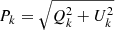
Following the notation of PR06, the polarization degree P and the polarization angle χ are related to the Stokes parameters by
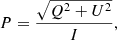 (1)
(1)
 (2)
(2)
Hereafter, we use Q ≡ Q/I and U ≡ U/I.
The polarization optics of dual-beam polarimeters, such as FORS2, allow us to measure simultaneously the intensities of two perpendicular components of the incident light beam, split by a Wollaston prism (WP, see Fig. 1). This measurement can be made at different position angles θi of the rotatable half-wave plate (HWP) that is placed before the WP. These two intensities are called ordinary fO, i and extraordinary fE, i beams (o and e beams)4, and the total intensity I of the source is related to fO, i and fE, i by I = fO, i + fE, i.
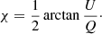
As discussed in PR06, the same field is observed at a minimum of four HWP positions chosen at constant intervals of Δθ = π/8 to minimize the errors. In this case the normalized Stokes parameters can be obtained from
 (3)
(3)
where each Fi, defined as the normalized flux difference at the position angle θi, is given by
 (4)
(4)
It is worth mentioning that by adopting normalized flux differences, atmospheric variations are canceled out. Thus, Fi can be written as
 (5)
(5)
Finally, the absolute uncertainty on the polarization degree, σP, and the uncertainty on the polarization angle, σχ, can be estimated following the procedure of PR06, namely
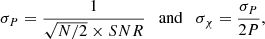 (6)
(6)
where SNR is the signal-to-noise ratio of the intensity, I = fO + fE. In Appendix B we present an alternative way to estimate the error on the polarization degree and angle based on a Fourier analysis.
A correct estimation of the polarization of a given light source requires the control of any spurious instrumental polarization. The goal is to understand the possible origins of the instrumental polarization and to develop a methodology to correct for it. In the next chapters we describe the different steps needed for the reduction and analysis of polarimetric data in FORS2.
3. FORS2 instrumental characterization
The FORS2 is a multi-mode optical instrument mounted on the Cassegrain focus of the UT1 telescope at ESO VLT. It works in the wavelength range 330 − 1100 nm. In imaging polarimetry (IPOL) mode, the linear or linear–circular polarizations of the incident light can be measured by employing a half-wavelength or quarter-wavelength plate, respectively. With the standard resolution (SR) collimator, 2 × 2 binning, the plate scale corresponds to 0.25″ pixel−1 and to a field of view (FoV) of 6.8′ × 6.8′ imaged onto two identical CCD detectors (CHIP1 and CHIP2). In this section we describe the data used to characterize the instrumental polarization across the FoV of FORS2. A particular emphasis is given to the different steps in the analysis of imaging linear polarimetry of extended sources.
3.1. Data
We acquired observatory technical time to characterize the instrumental polarization across the field of FORS2. The data were obtained during bright time (100% lunar illumination at ∼18° from the Moon) on 12 March 2017 (between 1:00 and 2:00 UT). The moonlit sky is expected to be highly polarized with a roughly constant value across the FoV. We targeted a blank field that is used for sky flats, α(J2000) = 10h04m26 98 and δ(J2000) = −02
 19′00.26″, ensuring that we obtained a high signal (i.e. > 30 000 counts per pixel). We observed the field with eight HWP position angles (θi = 0°, 22.5°, 45°, 67.5°, 90°, 112.5°, 135°, and 157.5°) observed in four filters, bHIGH, vHIGH, RSPECIAL, IBESS (corresponding to ESO filter numbers 113, 114, 76, and 77), hereafter BVRI, with exposure times per HWP angle position of 200, 120, 100, and 135 seconds, respectively.
Additionally, we used an independent way to measure the spatial instrumental polarization with the help of individual mostly unpolarized stars across the field. For this, we also acquired data for the cluster M 30 on a moonless night, at α(J2000) = 21h40m22 12 and δ(J2000) = −23°10′47.5″, with four HWP angles (θi = 0°, 22.5°, 45°, and 67.5°) in three different filters, HAlpha, RSPECIAL, and IBESS (corresponding to filter numbers 83, 76, and 77), hereafter HαRI under the program 0101.D-0142(A) (PI: Wiersema). The cluster was observed with different small offsets (from three to five) in the y-direction to maximize the number of stars. Both datasets were taken with the red sensitive MIT CCD and with a 2 × 2 binning.
Finally, to test the stability of our results, we also used archival IPOL data of unpolarized and polarized standard star fields: BD-12-5133, HDE-316232, Hiltner-652, Vela1, WD-0752-676, WD-1344+106, WD-1544-377, WD-1620-391, WD-2149+021, and WD-2359-434.
3.2. Reduction steps
In Fig. 2, we summarize the sequence of steps needed for the reduction of imaging polarimetric data of extended sources. Every raw image taken at each HWP angle is bias subtracted and corrected for cosmic rays (van Dokkum 2001). We then separate the o and e beams in each CCD using the strip mask (see Sect. 3.3) and combine the two chips (see Sect. 3.4). We then match the o- and e-beam positions with the method described in Sect. 3.5. We provide a way to apply a polarimetric “flat correction” in Sect. 3.6. The Stokes parameters need then to be corrected for the instrumental polarization values (Sect. 4.1) in order to obtain the polarization degree and angle (Sect. 4.2). The final steps include the chromatic correction of the zero angle of the HWP, which induces a non-negligible rotation in the polarization angle (see FORS2 manual and Bagnulo et al. 2009), as well as the correction for the known polarization bias (Serkowski 1958; Wardle & Kronberg 1974), which tends to overestimate low values of P with poor S/N. We use here the correction proposed by Plaszczynski et al. (2014). We have made all of our software publicly available5.
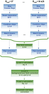 |
Fig. 2. Flow chart of the different steps required for the reduction of imaging polarimetric data of extended sources with FORS2. Blue boxes indicate steps applied to every θHWP, while green boxes require all HWP angles. |
3.3. Strip mask
In imaging polarimetry mode a strip mask is placed at the focal plane. This configuration avoids the superposition in the CCD of the two orthogonal polarized beams exiting from the birefrigent quartz WP. The strip mask is the odd numbered multi-object spectroscopy (MOS) mask of 22″ wide slits (see Fig. 3). In principle, a full coverage of an extended source thus requires a minimum of two images displaced by 22″, although three images are optimal as light gets lost at the mask edges due to diffraction effects. For observations of single point sources, the target is usually placed in the optical axis (located at the bottom of CHIP1) and requires neither strip mask nor offset exposures.
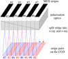 |
Fig. 3. Schematic representation of the strip mask placed on the focal plane before the polarization optics and the resulting ordinary and extraordinary beam pairs on the CCD. Taken from the FORS2 manual. |
The two polarization states of light split by the WP appear separated along the y-direction of the CCD in about 90 pixels. We thus measure the strip y positions for every single raw image of our moonlit and cluster observations by finding large abrupt changes in the light intensity gradient. We find no differences in the strip position for different HWP angles of a given filter. However, by summing all HWP images for a given filter, we do find variations in strip positions with wavelengths of up to ∼3 pixels. We confirm this for several other fields of standard stars. This is expected as the refractive indices of the quartz are wavelength dependent, affecting the positioning of the strips on the CCD6. We list the final strip positions for all BVRIHα filters in Table 1. Although variations of these positions are expected as the mask and/or instrument are removed and re-inserted, we only find ≲2 − 3 pixel deviations in other standard star fields. For more precise positions on a case-by-case basis, we recommend the gradient change approach that we follow here and that we released with our pipeline.
Strip y positions in pixels for the two chips in all BVRIHα filters.
3.4. Combining chips
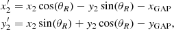
Since the FORS2 data consists of mosaics of two images from two CCDs or chips, we need to combine them to study extended sources. We briefly highlight here the procedure. First of all it is important to note that in addition to the CCD gap in y of yGAP = 480 μm (32 pix), there is also a shift in x of xGAP = 30 μm (2 pix) and also a slight angle (θR = 0.083°) between the two chips. This requires a rotation and a translation, which we perform on the second chip, CHIP2.
If x2 and y27 are the coordinates in CHIP2 in μm, using a pixel size of 15 μm, the simultaneous rotation and translation consist of
 (7)
(7)
where  and
and  are the new positions of CHIP2. The flux at those new positions are found via cubic 2D interpolation. We checked that the interpolation conserves the input signal well within the estimated flux uncertainties. After the combination of the two chips, the new reference point (x = 0, y = 0) lies at the bottom left pixel of the combined image. The typical position of the optical axis where a point source is usually observed lies at x0 = 1226 pix and y0 = 1025 pix of the combined image.
3.5. Matching the beams
After obtaining the combined images of the o and e beams, it is necessary to accurately match the coordinates of the ordinary and extraordinary beams corresponding to the same sky positions. This is required in order to measure the corresponding polarization in each position. In principle the position in x should be the same, while the shift in the y position is expected to be on the order of the width of each strip (i.e. around 90 pixels). Given that the refractive index of the WP changes with wavelength, we might expect this shift in y to change with filter as well.
In the case of point sources, the source can be used directly to find the shift between the o and e beams. To determine this for extended sources, we take advantage of the field stars by matching the brightest stars found in each of the two beam images of all of our M 30 cluster and Vela images. We use DAOFIND (Stetson 1987) for PYTHON and take the closest match in x and y positions for each star, ensuring that they do not exceed Δx < 10 pix and Δy < 150 pix to avoid incorrect matches. We show an example in Fig. 4 where we can see that, as expected, Δx < 1 pixel. Instead, the difference in Δy ∼ 90 pixels is not constant across the CCD, but increases by up to ∼3 − 7 pixels depending on the filter and as one moves towards the top of the combined image. Although the angular separation between the beams (arising from the difference in refractive indices) is constant, its corresponding spatial projection in the vertical plane of the CCD varies. We find that this difference is very closely approximated by a quadratic form,
![Mathematical equation: $$ \begin{aligned} \Delta y [\mathrm{pix} ]= (y_{\rm O}-y_{\rm E}) = a+b\,(y_{\rm O}-450)^2, \end{aligned} $$](/articles/aa/full_html/2020/02/aa36379-19/aa36379-19-eq13.gif) (8)
(8)
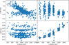 |
Fig. 4. Difference in o- and e-beam position, xdiff = xO − xE (top) and ydiff = yO − yE (bottom), for matched stars of ordinary and extraordinary beams as a function of o beam xO (left) and yO (right) location in the combined image. The results correspond to 583 stars of a M 30 I-band image at θHWP = 22.5°. The best quadratic fit for ydiff vs y is shown in orange. |
where a and b are free parameters in the fit and yO and yE are the pixel positions of the ordinary and extraordinary beams, respectively. This behavior is not symmetric about the center of the FoV, but increases from bottom to top forming a single quadratic form. We do not see any variation in the parameters with respect to the HWP angle, but we find an evident shift with filter coming from the wavelength dependence of the refractive indices of the WP. The final parameters for each filter are given in Table 2. We find these to be very robust (Δy < 1 pix) across different analyzed fields and epochs. Finally, we also note that there is a slight trend of Δy and Δx with x position, perhaps due to geometrical effects in the optics, but this is always below 0.5 pixel, which is within the error on the pixel position and much less than the typical PSF of the image and can thus be ignored. All of our e-beam image positions are matched to the corresponding o-beam positions through the relation given in Eq. (8), so that later fluxes in each beam can be compared and polarization analysis carried out.
Quadratic parameters to match y positions of ordinary and extraordinary beams for filters BVRIHα.
3.6. Polarization flat
In dual-beam polarimetry, the flat-fielding correction is a challenging task. Since the beam is split after optical components like the focal mask, the collimator, and the HWP, flats need to be taken with these elements in the light path. However, sources like internal flat screens and twilight sky may introduce polarization that is difficult to eliminate. In principle, this polarizing effect can be mitigated by obtaining dome screen flats with a continuously rotating HWP, so that the rotation is faster than the exposure time (see, e.g., Wiersema et al. 2018). As this is not possible for FORS2, we constructed depolarized flats by summing all HWP angles for the combined and matched o and e beams,
 (9)
(9)
where i corresponds to the index the HWP position angle.
In the ideal case, the fO and fE flats should be equal under uniform illumination of the field. We thus use here our blank field observations during the full moon, which for a given filter have essentially constant illumination. In Fig. 5 we show the polarization flat-field, defined as the ratio of the summed angles in o to e beam defined above: flat = fO/fE. Differences in the corresponding o and the e beams might indicate deviations of the WP from uniformity. Thus, this flat can be used to correct the beam intensities before calculating the flux differences (Eq. (4)) and the Q and U Stokes parameters (Eq. (3)).
 |
Fig. 5. Binned (30 × 30 pixel) polarization flat: sum of ordinary beam in 8 HWP angles divided by the sum of extraordinary beam in 8 HWP angles for a moonlit blank sky field in V band (left) and R band (right). |
We see that the flat-field may induce a 2% correction at the edge of the field. However, when we apply this flat correction before measuring the polarization, we find no significant difference in the maps of polarization degree and angle (see next section) due, in part, to the redundancy of multiple N = 8 HWP angles. However, by doing a careful Fourier analysis in Appendix B, we find that the flat correction reduces the errors in the polarization degree arising from secondary harmonics down to ≲0.4%. In addition to this small effect, flat-fielding can also help to clip bad pixels from a background measurement. Because it is taken at the same instrument position, such a flat is also useful to correct for fringing; this effect is generally small for FORS2, but it could become more important at longer wavelengths, for example, in filter z or with different detectors like the blue-sensitive E2V CCD, which is known to present more fringing. We therefore advise to perform the flat correction when dealing with extended sources.
4. FORS2 instrumental polarization with moonlit sky
The optical components of the telescope system and of the detector may induce instrumental polarization, as already highlighted for FORS1 (PR06). Disentangling the contribution of each component of the optical system for the total spurious instrumental polarization is a difficult task to simulate. In this section, we report on experimental tests and observations that can bring out the characteristics of the spurious instrumental polarization in the FoV of FORS2.
4.1. Background polarization
One way to estimate large-scale instrumental polarization is by measuring the moonlit sky polarization during full moon. The small FoV of the FORS2 ensures a roughly constant polarization of the moonlight along the image. The moonlit sky polarization depends on the separation of the observed target to the Moon and on the observing date and time. Observations of small fields (Wolstencroft & Bandermann 1973) and simulations of single Rayleigh scattering predict less than 0.05% polarization variance in sky polarization within the FoV of the instrument. For this reason larger deviations from a constant polarization in the FoV are expected to be independent of the Moon and generated by the spurious instrumental polarization.
Throughout this section, we study the field polarization. We analyze it pixel by pixel and also in binned boxes of 30 × 30 pixels in fO, i, fE, i images to increase the S/N by measuring the 2σ clipped mean intensity of each box. We always find that the results obtained pixel by pixel are consistent with the binned values, also for different box sizes and clipping.
To estimate the instrumental polarization, we follow the methodology described in Sect. 3: all 16 images (2 chips in 8 HWP angles) of a given filter are first separated into o and e beams, chip-combined, and flat-field corrected; then we use the eight HWP angles to measure Q and U Stokes parameters with Eq. (3). In Fig. 6 we show the Q–U plane in R band. Clearly there is an overall shift of all points with respect to zero that is best represented by the median background value of all points, at QR ≃ 0.8% and UR ≃ −2.9%, which is very close to the value at the center of the FoV. This corresponds (from Eq. (1)) to a polarization of PR = 3.0%.
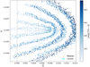 |
Fig. 6. Q–U plane for moonlit sky polarization in R band. Each point corresponds to a box of 30 × 30 pixels and the y position with respect to the center is colored in different shades of blue. The median value of Q and U is shown as an orange cross, while the value at the optical axis (x0 = 1226, y0 = 1025 pix) of the instrument is shown in cyan. Dashed lines indicate Q = 0. Typical errors on Q and U are on the order of 10−5 (see Table B.1). |
We note that using a simple Rayleigh scattering model of the Moon located at ∼17° from our blank target field (see Appendix A) predicts a background value of PB = 3.5%. All background values for our BVRI images are shown in Table 3. We analyze fields with different background polarizations in Sect. 6.
Background QB, UB, PB, and χB values of moonlit sky observations for BVRI filters.
To analyze the spatial characteristics of the instrumental polarization we must therefore correct for these background values before calculating the polarization degree and angle along the FoV using Eq. (1). In principle this background polarization corresponds to the central value (i.e., at the telescope optical axis), but in fields with sources in the center the correction with the median is more appropriate. We thus do a vectorial correction of the observed polarization,
 (10)
(10)
where QB and UB are the background median values.
Alternatively, by substituting this into Eq. (1), the measured polarization parameters (P, χ) corrected for the background values (PB, χB) are given by
![Mathematical equation: $$ \begin{aligned} P_{\mathrm{corr} }&=\sqrt{P^2+P_B^2-2PP_B\cos {(\chi -\chi _B)}} \\ \chi _{\mathrm{corr} }&=\arctan {\left[\frac{P\sin {\chi }-P_B\sin {\chi _B}}{P\cos {\chi }-P_B\cos {\chi _B}}\right]}\cdot \nonumber \end{aligned} $$](/articles/aa/full_html/2020/02/aa36379-19/aa36379-19-eq16.gif) (11)
(11)
However, even before correcting for the background polarization, we can already see in the uncorrected Q–U plane of Fig. 6 that there is a net increase in the Q and U parameters as we move away from the optical axis. We note the y-strip map structure that produces the empty spaces in the Q–U plane. We show the Q and U maps after correcting for the background values in Fig. 7 for the B band. The Q and U patterns are both closely approximated by a hyperbolic paraboloid (a “saddle”) of the form
![Mathematical equation: $$ \begin{aligned} Q(x,y),U(x,y) =&\frac{[y^{\prime }(x,y)]^2}{b^2} - \frac{[x^{\prime }(x,y)]^2}{a^2} \\ \nonumber =&\frac{[(x-x_0)\sin \theta +(y-y_0)\cos \theta ]^2}{b^2} \\ \nonumber&-\frac{[(x-x_0)\cos \theta -(y-y_0)\sin \theta ]^2}{a^2}\cdot \nonumber \end{aligned} $$](/articles/aa/full_html/2020/02/aa36379-19/aa36379-19-eq17.gif) (12)
(12)
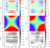 |
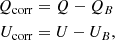
Fig. 7. Top: binned Q (left) and U (right) maps in B band after correction for the background value. Middle: hyperbolic paraboloid fit using Eq. (12) and parameters in Table 4. Bottom: residual of observed map minus the fit. |
The paraboloid is described by the free a and b parameters (different for Q and U), whereas x0 and y0 represent the central position where Q, U = 0, and θ determines the rotation of the paraboloid in the xy plane, so that  . Such a 2D fit and residual map are also shown in Fig. 7. All residuals are below 0.06% for Q and U. We present the resulting fit parameters for BVRI in Table 4. The analytic maps can be used to correct the spatial instrumental polarization.
Although practical and convenient, analytic functions may not capture all small-scale variations and might lead to artificial features that are not really present. We therefore also perform non-analytic fits in Sect. 4.3 finding residuals that are one to two orders of magnitudes lower.
4.2. Polarization map
After correcting for the background polarization, we map the polarization and polarization angle along the FoV. We do this pixel by pixel and in 30 × 30 pixel bins. The results for this field instrumental polarization are shown in Figs. 8 and 9.
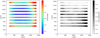 |
Fig. 8. Map of polarization degree (left) and error (right) for V band calculated pixel by pixel for the moonlit sky with eight HWP angles, after correction for the background value. |
 |
Fig. 9. Map of polarization angle (left) and error (right) for V band calculated pixel by pixel for the moonlit sky with eight HWP angles, after correction for the background value. |
The radial pattern is quite clear in the polarization map increasing from nearly zero in the central telescope optical axis up to ∼1.4% at the boundary depending on the filter. This can also be seen in Fig. 10 where we show the radial profile together with some polynomial fits. We find that the behavior is accurately represented by a cubic polynomial,
 (13)
(13)
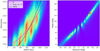 |
Fig. 10. Two-dimensional histogram of polarization vs radius (left) and polarization angle vs arctan(y/x) (right) for all pixels in the moonlit sky in I band for FORS2. Shown are the radial fits of a cubic polynomial with and without forcing P(r = 0) = 0 (pink dashed and solid lines, respectively). The radial fit for FORS1 from PR06 is also shown (black line). |
with m1, 2, 3 parameters for each filter given in Table 5 and with the radius,  , given in pixels. We note that these parameters are in good agreement with FORS1 (PR06), as expected if this large-scale pattern in the spurious polarization stems from the curved collimator lenses which are identical in FORS2. The distribution of polarization angle as a function of polar angle in the right Fig. 10 further emphasizes that the pattern is strongly radial.

Although the radial 1D fit helps understand the behavior of the instrumental polarization as we move towards the extremities of the FoV, a better approximation should take the azimuthal variation into account as well. This can be done directly with the corrected Q and U Stokes parameters calculated in the previous section or, alternatively, we can perform a 2D fit to the polarization degree with a paraboloidal function, which has the freedom of having the axes rotated, as follows:
![Mathematical equation: $$ \begin{aligned} P(x,y) =&\frac{[x^{\prime }(x,y)]^2}{a_P^2} + \frac{[y^{\prime }(x,y)]^2}{b_P^2} \\ \nonumber =&\frac{[(x-x_{0,P})\cos \theta _P-(y-y_{0,P})\sin \theta _P]^2}{a_P^2}\\ \nonumber&+ \frac{[(x-x_{0,P})\sin \theta _P+(y-y_{0,P})\cos \theta _P]^2}{b_P^2}\cdot \nonumber \end{aligned} $$](/articles/aa/full_html/2020/02/aa36379-19/aa36379-19-eq22.gif) (14)
(14)
The paraboloid is described by the free aP and bP parameters, whereas x0, P and y0, P represent the coordinates of the central P = 0 position (with respect to the telescope optical axis) and θP determines the rotation of the paraboloid in the xy plane. These fits and residuals are shown in Fig. 11 for filters V and I, while all final parameters are presented in Table 6. We can see that the rotated paraboloid can remove most of the polarization pattern with residuals below P ∼ 0.05%, which is within the estimated error (see Appendix B). The most asymmetrical pattern is found for B and V bands in agreement with the results of PR06 for FORS1. These asymmetries can be seen directly in the polarization map obtained from the corrected Q and U or via non-analytic fits, as shown in next subsection. The origin of this asymmetrical polarization is unknown.
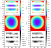 |
Fig. 11. Binned polarization map (top), rotated paraboloidal fit of Eq. (14) (middle), and residual between the two (bottom) for filters V (left) and I (right) of moonlit sky. |
4.3. Non-analytic map: INLA model
We use here a non-analytic fitting procedure to obtain maps of the Stokes parameters, Q and U, the polarization degree, P, and angle, χ, of the FORS2 instrument optics in BVRI obtained from the same moonlit blank fields investigated in the previous sections. In principle this allows a reconstruction that is less subject to forced features from the assumed analytic function. We use a method based on Gaussian Markov random fields to model the underlying continuous spatial field with hyper-parameters fitted with a Bayesian inference algorithm known as the integrated nested Laplace approximation (INLA, Rue et al. 2017). The method offers the additional advantage of full posterior distributions to properly model uncertainties. INLA has been successfully applied in many different areas including extended sources in astronomy (González-Gaitán et al. 2019).
Although at first the INLA reconstructions of Q and U look quite similar to the analytic hyperbolic paraboloid, the residuals in B band are at least one order of magnitude smaller and show no clear patterns, as opposed to the analytic fits. The advantage of the INLA fits becomes more evident in the polarization fits shown in Fig. 12, where the asymmetric behavior is clearly visible in the reconstruction, and it is confirmed in the rather flat residual map. We present the median and deviation of all residual maps in Table 7. We also release all final INLA reconstructions8.
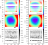 |
Fig. 12. Binned polarization map (top), INLA fit (middle), and residual between the two (bottom) for filters V (left) and I (right) of moonlit sky. |
Median and median absolute deviation of the residual maps for the INLA fits of Q, U, P, and χ.
We present in this section analytic and non-analytic spatial corrections for the spurious instrumental linear polarization of broad-band filters. In the following sections we validate these results with other datasets.
5. FORS2 Instrumental polarization with a star cluster
In this section, we use independent observations of the stellar cluster M 30 to test the maps of instrumental polarization found in the previous section. M 30 observations were performed with several ditherings in broad-band filters RI and in the narrow Hα filter. Containing hundreds of stars across the field, we can validate the spatial instrumental pattern by performing stellar photometry in the images taken in each HWP angle and then applying the same formalism presented in Sect. 2 to measure the polarization of each individual star. This independent method offers some benefits: we can test whether the spurious instrumental polarization persists in a field with mostly unpolarized sources and no strong background polarization; it also permits us to study the effects of ghosting, vignetting, point spread function (PSF) variations across the field and between o and e beams (see, e.g., Clemens et al. 2012). The disadvantages, in addition to the difficulties of performing crowded stellar photometry, is the possible presence of varying interstellar dust polarization across the field, and foreground and background stars with polarization degrees that differ from the M 30 member stars.
5.1. Field polarimetry
As a first simple step, we use the same methodology as for the moonlit sky (Sect. 4), now applied to the M 30 cluster: we bin each image in boxes of 30 × 30 pixels and calculate Q, U, P, and χ. It is important to note that in this first step we do not perform any stellar photometry. Even though the S/N at each pixel is not as high as for the bright moonlit sky, Fig. 13 shows a similar radial instrumental pattern in R band (after correction for the median background Q and U). This pattern is confirmed for all pointings of R and I. If we apply the spatial correction for the Q and U maps that we obtained from the hyperbolic paraboloid fits (see Table 4), we find a roughly flat map, except for the center where the crowded nucleus of the stellar cluster leaves a residual polarization. This demonstrates the validity of our instrumental correction.
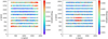 |
Fig. 13. Polarization map for a field with M 30 in R for binned (30 × 30 pix) boxes (left) and after spatial field correction in Q and U using Eq. (12) (right). The residual central polarization from the cluster center can be seen. |
5.2. Stellar polarimetry
Now we turn to the more difficult task of doing photometry for crowded fields of each o- and e-beam image of all the HWP angles at different offsets. Due to the high density of the sources, the aperture photometry for stellar clusters is generally inaccurate and PSF modeling is required. For this we use a general PSF template across the field built from a set of bright stars. To avoid systematic biases, we use the same PSF for all HWP angle exposures of a given offset and filter. The sources are found by selecting significant brightness peaks above the background, which are then fitted to the PSF model and subtracted. The process is repeated to find any leftover sources. All steps are included in the packages PHOTUTILS9 in PYTHON or STARFINDER in IDL (Diolaiti et al. 2000). When doing photometry it should be kept in mind that the background subtraction may eliminate some of the polarization pattern. Our tests with and without subtraction are consistent throughout.
To match the star catalogs of different HWP angles, we look for the closest star within 1 pixel in x and y positions. We then calculate the Q and U Stokes parameters from Eq. (3) and the polarization from Eq. (1) for each star. We show in the left Fig. 14 the resulting star polarization degree for M 30 in R band. This figure includes three different pointings with the center slightly offset and a total of more than 13 000 star positions. Because of the multiple pointings of the same field, many stars are repeated, yet at various locations in the field. The scatter in the polarization of stars is very large; we therefore bin the individual star Q, U values into boxes of 20 × 20 pixel boxes, rejecting 2σ outliers, and calculate the polarization within each box, as shown in the middle plot. We can see here a radial pattern similar to Fig. 13, which we correct with the hyperbolic paraboloid function and parameters found with the moonlit observations, thus removing some of the spurious edge polarization and obtaining a flatter pattern (right plot). This is also consistent with the moonlit sky approach, and argues for an instrumental field polarization that is valid for both polarized and unpolarized incoming light.
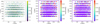 |
Fig. 14. Individual stellar polarization map for M 30 of three combined pointings in R (left) and binned in 20 × 20 boxes (middle) and after spatial field correction in Q and U using Eq. (12) (right). The binned maps have a characteristic polarization error of ∼0.4%. |
We emphasize however that the correction is not optimal with a large scatter in the distribution of degrees of star polarization. This may come from the large photometric uncertainties obtained from PSF photometry in very dense clusters. Doing aperture photometry instead, or restricting the analysis to only a fraction of stars with high S/N, does not reduce the scatter. This is noted by Clemens et al. (2012), who ultimately perform precision photometry by first removing stars from around a target star using PSF stellar fits, then doing aperture photometry on the target star, and iterating this procedure for new target stars. This approach is beyond the scope of this paper.
5.3. The case of the narrow Hα filter
At first sight it might be expected that the behavior of the spatial instrumental pattern extends to other wavelengths not explored with the bright sky observations, so that a simple interpolation of the paraboloid parameters to the effective wavelengths of other filters should suffice. However, the narrow-band interference filters are in the converging beam and not the collimator, as is the case for the broad-band filters. If the primary spurious pattern is due to the curved lenses in the collimator, the question arises of whether this affects the instrumental pattern. We try here to explore this with our observations of M 30 in the Hα filter at four HWP angles and three different pointings. By doing a similar analysis to that used for R and I, we first find that in a binned analysis (see Fig. 15) there is no apparent radial pattern. However, this is within the inferred error which is on the order of ∼10% in polarization. Although quite low, this S/N is only roughly a factor of 2 lower than for the broad-band filters where the pattern is clearly seen. This is confirmed for all three M 30 pointings and for an additional standard star field10, although all with low S/N.
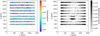 |
Fig. 15. Binned Hα polarization map for M 30 at a single pointing (left) and error (right). |
Using stellar PSF photometry, our results look similar to the broad-band filters (see Fig. 16): the polarization degree seems to increase towards the outer parts of the CCD in agreement with the instrumental pattern found at other wavelengths of broad-band filters. However, the degree of polarization is lower compared to the broad bands (up to ∼0.9% versus 1.4%), and when correcting for the instrumental pattern found previously, we do not obtain lower residuals in the polarization map. Although the S/N is low, even after binning individual Q, U star values, the scatter is large suggesting again that a more robust photometry technique should be applied or that a higher S/N is needed.
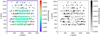 |
Fig. 16. Hα star polarization degree map for M 30 in three pointings binned in 20 × 20 boxes (left) and respective error (right). |
6. Stability of the instrumental polarization
In this section we briefly discuss some biases that may affect the stability of the instrumental polarization pattern found in the previous sections.
First, there is a known effect of cross-talk in FORS2 in which linear polarization creates a non-negligible circular polarization (Bagnulo et al. 2009). On-axis, the induced circular polarization is quite low for unpolarized sources (≪0.01%), and increases for highly polarized objects (∼0.5% for 10% polarization). Since the spatial linear instrumental polarization increases with off-axis distance, it is expected that this cross-talk might increase as well. These authors (see their Table 1) find an increase in the circular polarization cross-talk by a factor of roughly ∼1.2 to the edge of the detector. This corresponds surprisingly well with the radial increase in linear polarization that we find in this work, which could thus partly explain their findings. Although we neglect the study of circular polarization here, the question arises whether the instrumental pattern changes, for instance, with varying background linear polarization. Although the study of unpolarized cluster stars in a moonless night (see previous section) suggests that the spatial instrumental pattern is global, more observations with different background polarizations are advisable.
Furthermore, there may be some concerns about telescope flexure. It is known that there is image motion due to instrument flexure under gravity below 0.25 pixel over a one-hour exposure with the SR collimator for zenith distances less then 60° (see the FORS2 manual). Although this is rather small, the effects on the spurious linear polarization pattern are still unknown.
Finally, a natural concern is that our corrections may evolve with time. For instance, as coatings age or are changed, as mirrors get re-coated, or as the instrument is unmounted and mounted again, there may be variations in the induced instrumental pattern. Wiersema et al. (2018) find for example a time-dependent effect on the calibration of the instrument EFOSC2 due to oxidation, dust, and perhaps other factors, settling on the tertiary mirror of the NTT.
To gauge some of these concerns, since our moonlit sky observations were taken only at one pointing, we investigate here the instrumental polarization for other targets with different Moon separations and therefore varying background polarization degrees and angles. We study several fields observed with FORS2-IPOL in BVRI available from the ESO archive. The data were obtained at different dates and times and thus at varying background linear polarizations, telescope elevations, among others. Most of these data come from standard star fields observed in linear polarimetry mode and have much lower signal-to-noise ratios compared to our moonlit sky observations. In Fig. 17, we show binned Q, U, and P for four different fields at different epochs. Albeit with lower S/N, we can recognize the pattern found previously. When we correct with the analytic paraboloid functions, we obtain residual maps on the order of ∼10−4, lower than the typical intrinsic error of ∼10−2.
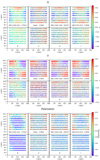 |
Fig. 17. Binned Q (top two rows), U (middle two rows), and P maps (bottom two rows) after correction for median Q0, U0 values (top) and after correction of instrumental field polarization from paraboloid fits of Sect. 4 (bottom) for standard star fields of (a) WD-2149+021 at Modified Julian Date (MJD) of 57919 in B band, (b) Vela1 at MJD = 57845 in V band, (c) WD-1344+106 at MJD = 58278 in R band, and (d) WD-0752-676 at MJD = 57846 in I band. |
Furthermore, if we perform individual paraboloid fits for each of the cases we retrieve from the archive, we obtain quite consistent fit parameters (see Fig. 18) and find no evidence of variation with observation date nor altitude and/or azimuth of the target. The data we investigate spans observations from 2011 until 2018 suggesting that there is not a significant time evolution of the instrumental linear polarization. This is confirmed by the similar pattern found already by PR06 for FORS1 (see Sect. 4). We also do not find changes with background sky polarization (which is always corrected for prior to the fit), but there is some scatter and only few observations with high polarization. We also see that when the intensity has S/N ≲ 10, the obtained parameters drift off from the median values for all Q, U, and P parameters. This finding suggests a minimum signal-to-noise cutoff for reliable spatial linear polarization studies. For low polarization degrees (i.e. P ≲ 0.03) this S/N corresponds to P/σP ≲ 0.5, a value much lower than the typical 3σ limit to consider real linear polarization detections (e.g., Manjavacas et al. 2017). Finally, it is important to mention that although the fit parameters are mostly consistent, a few outliers exist, even though they have decent S/N and low background polarization. The origin of this discrepancy is unknown.
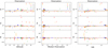 |
Fig. 18. Paraboloid fit parameters aP (top), bP (middle), and θP (bottom) of Eq. (14) for the polarization degree of multiple FORS2 fields as a function of target altitude (left), median background polarization degree (middle) and intensity S/N (right). Different filters are color-coded, and filled circles represent our moonlit sky observations. Dashed horizontal lines are the median of the parameters per filter. |
The changes in the spatial instrumental linear polarization therefore need to be studied further with high signal-to-noise observations, ideally with moonlit sky observations (as in Sect. 4) at different telescope elevation angles and Moon separations (i.e. at different background sky polarizations). This would better clarify the stability of the instrumental polarization pattern under different observing conditions. By adding circular polarization measurements, it will be possible to address the question of possible cross-talk in a more systematic way.
7. Summary
We presented a detailed study of the spatial instrumental polarization of FORS2 at VLT in imaging polarimetry mode for broad-band filters BVRI. We also explored it for the narrow-band filter Hα. By studying moonlit sky blank fields and the stellar cluster M 30, we find a radial instrumental pattern that is in good agreement with previous results for the decommissioned twin instrument FORS1 (Patat & Romaniello 2006) in the broad-band filters. The radial behavior is expected from the effect of the curved lenses of the collimator. The origin of some minor asymmetrical features, particularly in the B band, remains unknown. We provide analytic equations to correct the Q and U Stokes parameters and the polarization in each band down to a ∼0.05% level. We also release non-analytic INLA maps that enable a better correction of asymmetrical components down to ∼0.02%. All reduction and analysis software, maps, and results of this analysis are released.
We also presented important tips and tricks to be taken into account in the reduction and analysis of polarimetric measurements of extended sources. We find for instance a variation in the mask strip positions in the CCD as a function of wavelength, and more importantly an increasing shift between o- and e-beam positions throughout the field that is well represented by a quadratic form. These effects come from the geometry of the Wollaston prism and the wavelength dependence of its refractive indices. We also present a way to correct for flat-fielding in polarimetric observations by summing the images in all HWP angle positions of a given band.
The spatial polarization correction is vital in polarimetric studies of extended sources such as galaxies, clusters, nebulae. We have provided here the pathway for accurate corrections to an accuracy much below the typical estimated error in FORS2 at VLT. Although our initial studies suggest that the spatial instrumental linear polarization is stable, further studies of this kind at different observing conditions are encouraged to fully characterize its stability. Finally, the methodology presented in this study can be applied to polarimetric measurements using other dual-beam polarimeters.
FORS2 is largely identical to FORS1, particularly its geometry and optical components, except for some modifications like grisms of higher resolution and coatings.
Although see the effect of cross-talk in Sect. 6.
According to the FORS2 calibrations, when the HWP is at the zero position angle, the light from a point source is split into two beams in such a way that the component polarized along the meridian, called the ordinary beam (o beam), falls in the upper part of the xy plane of the CCD, whereas the beam with perpendicular polarization, called the extraordinary beam (e beam), reaches the CCD in the same column (x position) but a lower row (y position). The position angle of the HWP is measured relative to the meridian. The terms “fast” and “slow” are also used to distinguish between the two out-coming perpendicularly polarized beams affected by lower and higher refractive indices in the WP and the HWP.
Although the full analysis of the optical system is beyond the scope of the paper, in a simple treatment the refractive indices of fuse quartz (SiO2) change between 1.4663 at 440 nm in B band to 1.4539 at 768 nm in I band (Malitson 1965) which leads to an outgoing angle difference of less than a degree and a corresponding vertical shift of up to 10 pixels at the edge the field.
There is a pre- and over-scan region for both chips of FORS2 of 5 pixels in y, which we previously removed.
Vela1 at Modified Julian Date = 58281, see Sect. 6 for the analysis of standard star fields.
Acknowledgments
We thank the anonymous referee for the valuable comments that improved the paper. We thank José Lopes for some of the diagrams of this paper. The authors acknowledge B. Leibundgut, G. Rupprecht and T. Szeifert for important clarifications regarding the characteristics and calibrations of FORS2 in IPOL mode, V. Ivanov for important discussions regarding data reduction, and S. Moehler for carefully reading the manuscript. A. M. thanks her colleagues at the Department of Physics, Instituto Superior Técnico, namely P. Brogueira, I. Cabaço and C. Cruz for the very useful discussions about properties of crystals and G. Figueira for the tests with polarized light and a half wave plate. A. M. also thanks ESO for the hospitality and stimulating atmosphere and FCT – Fundação para a Ciência e Tecnologia for the financial support during her sabbatical leave at ESO. This work was supported by FCT under Project CRISP PTDC/FIS-AST-31546. The authors thankfully acknowledge the computer resources, technical expertise and assistance provided by CENTRA/IST. Computations were performed at the cluster “Baltasar-Sete-Sóis” and supported by the H2020 ERC Consolidator Grant “Matter and strong field gravity: New frontiers in Einstein’s theory” grant agreement no. MaGRaTh-646597.
References
- Appenzeller, I., Fricke, K., Fürtig, W., et al. 1998, The Messenger, 94, 1 [NASA ADS] [Google Scholar]
- Bagnulo, S., Landolfi, M., Landstreet, J. D., et al. 2009, PASP, 121, 993 [NASA ADS] [CrossRef] [Google Scholar]
- Berry, M. V., Dennis, M. R., & Lee, R. L. 2004, New J. Phys., 6, 162 [NASA ADS] [CrossRef] [Google Scholar]
- Born, M., & Wolf, E. 1984, Principles of Optics, 6th edn. (New York: Pergamon Press), 808 [Google Scholar]
- Chandrasekhar, S. 1960, Radiative Transfer (New York: Dover), 393 [Google Scholar]
- Clemens, D. P., Pavel, M. D., & Cashman, L. R. 2012, ApJS, 200, 21 [NASA ADS] [CrossRef] [Google Scholar]
- Diolaiti, E., Bendinelli, O., Bonaccini, D., et al. 2000, A&AS, 147, 335 [NASA ADS] [CrossRef] [EDP Sciences] [Google Scholar]
- Fendt, C., Beck, R., Lesch, H., & Neininger, N. 1996, A&A, 308, 713 [NASA ADS] [Google Scholar]
- Gál, J., Horváth, G., Barta, A., & Wehner, R. 2001, J. Geophys. Res., 106, 22647 [NASA ADS] [CrossRef] [Google Scholar]
- González-Gaitán, S., de Souza, R. S., Krone-Martins, A., et al. 2019, MNRAS, 482, 3880 [NASA ADS] [CrossRef] [Google Scholar]
- Harrington, D. M., Kuhn, J. R., & Hall, S. 2011, PASP, 123, 799 [NASA ADS] [CrossRef] [Google Scholar]
- Heisenberg, W. 1958, Physics and Philosophy: The Revolution in Modern Science, World Perspectives, 19, 1 [Google Scholar]
- Hough, J. 2006, Astron. Geophys., 47, 3.31 [CrossRef] [Google Scholar]
- Malitson, I. H. 1965, J. Opt. Soc. Am., 55, 1205 [NASA ADS] [CrossRef] [Google Scholar]
- Manjavacas, E., Miles-Páez, P. A., Zapatero-Osorio, M. R., et al. 2017, MNRAS, 468, 3024 [NASA ADS] [CrossRef] [Google Scholar]
- McMaster, W. H. 1954, Am. J. Phys., 22, 351 [NASA ADS] [CrossRef] [Google Scholar]
- Momose, M., Tamura, M., Kameya, O., et al. 2001, ApJ, 555, 855 [NASA ADS] [CrossRef] [Google Scholar]
- Patat, F., & Romaniello, M. 2006, PASP, 118, 146 [NASA ADS] [CrossRef] [Google Scholar]
- Plaszczynski, S., Montier, L., Levrier, F., & Tristram, M. 2014, MNRAS, 439, 4048 [NASA ADS] [CrossRef] [Google Scholar]
- Reilly, E., Maund, J. R., Baade, D., et al. 2017, MNRAS, 470, 1491 [NASA ADS] [CrossRef] [Google Scholar]
- Rue, H., Riebler, A., Sørbye, S. H., et al. 2017, Annu. Rev. Stat. Appl., 4, 395 [CrossRef] [Google Scholar]
- Scarrott, S. M., Warren-Smith, R. F., Pallister, W. S., Axon, D. J., & Bingham, R. G. 1983, MNRAS, 204, 1163 [NASA ADS] [CrossRef] [Google Scholar]
- Serkowski, K. 1958, Acta Astron., 8, 135 [NASA ADS] [Google Scholar]
- Stetson, P. B. 1987, PASP, 99, 191 [NASA ADS] [CrossRef] [Google Scholar]
- Strutt, H. J. 1871, The London, Edinburgh, and Dublin Philosophical Magazine and Journal of Science, 41, 107 [CrossRef] [Google Scholar]
- van Dokkum, P. G. 2001, PASP, 113, 1420 [NASA ADS] [CrossRef] [Google Scholar]
- Wardle, J. F. C., & Kronberg, P. P. 1974, ApJ, 194, 249 [NASA ADS] [CrossRef] [Google Scholar]
- Wiersema, K., Higgins, A. B., Covino, S., & Starling, R. L. C. 2018, PASA, 35, e012 [NASA ADS] [CrossRef] [Google Scholar]
- Wolstencroft, R. D., & Bandermann, L. W. 1973, MNRAS, 163, 229 [NASA ADS] [CrossRef] [Google Scholar]
Appendix A: Rayleigh sky scattering
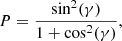
The method used in this work to calculate the instrumental polarization relies on the assumption that it is null in the optical axis and that we can therefore correct it, and that the night sky polarization is constant within the field of FORS2. To study this further, we use here a simple model of single Rayleigh scattering from the Moon (e.g., Strutt 1871; Harrington et al. 2011), simply described as
 (A.1)
(A.1)
where γ is the angle between the Moon and the target pointed by the telescope.
Although our observations were taken during a full Moon, throughout all of the exposures in all filters the angle from the Moon changed between 17.69° and 18.31°, which corresponds to a raw single Rayleigh scattering polarization of ∼3.51 − 4.69%. This is somewhat higher than the values we measure and quote in Sect. 4.1. We assume that this comes from our simplistic mono-chromatic model that does not take into account multiple scattering and proper atmospheric models. We show one of our simulations in Fig. A.1. It is important to see that in this model, the polarization degree from Moon scattering does not change more than 0.06% throughout the field of FORS2, a value that is below the expected polarization we can measure (see Appendix B). Even if the real pattern is more complicated when going beyond simple Rayleigh scattering (e.g., Gál et al. 2001; Berry et al. 2004), we do not expect the polarization to change substantially within the small angular scales of the FoV. Findings of constant sky polarization in small fields have been observed by others (Wolstencroft & Bandermann 1973).
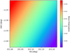 |
Fig. A.1. Simulated monochromatic single Rayleigh scattering model of the Moon at the location and time of our blank target observation with the FoV of FORS2. The polarization degree here is (3.51 ± 0.05)%. |
Appendix B: Fourier analysis
The Fourier decomposition allows for the identification of different sources of error, including instrumental components. The relation between the normalized flux differences and the Stokes parameters defined in Eq. (4) allows for such error analysis based on the Fourier transform. In the case of observations using N = 4, 8, 12, and 16 position angles of the HWP with a constant interval of π/8, the normalized flux differences, Fi in Eq. (4), can be rewritten as
 (B.1)
(B.1)
where Q0, Qk, and Uk are the Fourier coefficients.
From the Fourier coefficients, we can obtain the polarization of each harmonic (i.e. the polarization spectrum):
 (B.2)
(B.2)
Comparing the above formulae with Eqs. (3) and (4), it is possible to understand that the linear polarization signal is given by the k = N/4 harmonic, whereas the other components are related to different effects like instrumental imperfections and noise (Fendt et al. 1996).
The different components of the Fourier transform for our moonlit sky observations are presented in Figs. B.1 for B and B.2 for I. We have corrected all Qk and Uk components for the median value of the map. We can clearly see at k = 2 the same pattern for Q and U seen in Fig. 7, indicating as expected that this component carries the signal. All other harmonics have a much lower contribution. The k = 0 component, whose deviations from zero normally indicate anomalies with the WP, is reminiscent of the flat of Sect. 3.6. If we apply a flat correction prior to the Fourier analysis, the observed Q0 pattern almost disappears entirely going below Q0 < 0.003%. This demonstrates that although the final polarization degree is not significantly affected by a secondary flat correction, its minor contribution is clearly seen in the Fourier analysis. The k = 1 and k = 3 harmonics are quite different depending on wavelength: for B we find a contribution that rises up to 0.2% at the edges of the field, whereas in I no clear pattern is seen and the signal is below 0.05%. We attribute this partly to the pleochroic effect of the HWP that depends on wavelength. We also show the Pk maps in Fig. B.3.
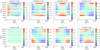 |
Fig. B.1. Binned (30 × 30 pixel) Fourier Qk and Uk coefficients for a moonlit blank sky field in B band. The color scale in each plot is different. All values have been corrected for median background Qk, B, Uk, B values. |
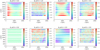 |
Fig. B.2. Binned (30 × 30 pixel) Fourier Qk and Uk coefficients for a moonlit blank sky field in I band. The color scale in each plot is different. All values have been corrected for median background Qk, B, Uk, B values. |
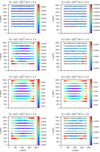 |
Fig. B.3. Binned (30 × 30 pixel) Fourier power spectra |
From the secondary harmonics (k ≠ N/4), we can also infer the error contribution:
 (B.3)
(B.3)
In Fig. B.4 we can see that the error budget on the polarization degree is less than 0.2% in B and less than 0.05% in I. The median value and median absolute deviation of the error maps are shown in Table B.1. Thus, the estimate based on the S/N (Eq. (6)), for example in Fig. 8, is larger and is a conservative upper limit. We also confirm that the error is clearly larger than any of the residuals of the various models to correct the instrumental polarization (Table 6).
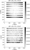 |
Fig. B.4. Binned (30 × 30 pixel) sum of the Fourier harmonics except k = 2, thus representing a characteristic error, ΔP, for a moonlit blank sky field in B band (top) and I band (bottom). This is after flat correction and median background Qk, B, Uk, B correction. |
Median and median absolute deviation (MAD) of the error maps obtained from the Fourier coefficients.
All Tables
Quadratic parameters to match y positions of ordinary and extraordinary beams for filters BVRIHα.
Background QB, UB, PB, and χB values of moonlit sky observations for BVRI filters.
Median and median absolute deviation of the residual maps for the INLA fits of Q, U, P, and χ.
Median and median absolute deviation (MAD) of the error maps obtained from the Fourier coefficients.
All Figures
|
Fig. 1. Schematic representation of a dual-beam polarimeter: an initial light ray with two polarization states (shown in blue and red) passes through a half-wave plate (HWP) and a Wollaston prism (WP) that splits it into two light beams with perpendicular polarization states. The optical axis in each of the two crystals of the WP is also shown. |
| In the text | |
|
Fig. 2. Flow chart of the different steps required for the reduction of imaging polarimetric data of extended sources with FORS2. Blue boxes indicate steps applied to every θHWP, while green boxes require all HWP angles. |
| In the text | |
|
Fig. 3. Schematic representation of the strip mask placed on the focal plane before the polarization optics and the resulting ordinary and extraordinary beam pairs on the CCD. Taken from the FORS2 manual. |
| In the text | |
|
Fig. 4. Difference in o- and e-beam position, xdiff = xO − xE (top) and ydiff = yO − yE (bottom), for matched stars of ordinary and extraordinary beams as a function of o beam xO (left) and yO (right) location in the combined image. The results correspond to 583 stars of a M 30 I-band image at θHWP = 22.5°. The best quadratic fit for ydiff vs y is shown in orange. |
| In the text | |
|
Fig. 5. Binned (30 × 30 pixel) polarization flat: sum of ordinary beam in 8 HWP angles divided by the sum of extraordinary beam in 8 HWP angles for a moonlit blank sky field in V band (left) and R band (right). |
| In the text | |
|
Fig. 6. Q–U plane for moonlit sky polarization in R band. Each point corresponds to a box of 30 × 30 pixels and the y position with respect to the center is colored in different shades of blue. The median value of Q and U is shown as an orange cross, while the value at the optical axis (x0 = 1226, y0 = 1025 pix) of the instrument is shown in cyan. Dashed lines indicate Q = 0. Typical errors on Q and U are on the order of 10−5 (see Table B.1). |
| In the text | |
|
Fig. 7. Top: binned Q (left) and U (right) maps in B band after correction for the background value. Middle: hyperbolic paraboloid fit using Eq. (12) and parameters in Table 4. Bottom: residual of observed map minus the fit. |
| In the text | |
|
Fig. 8. Map of polarization degree (left) and error (right) for V band calculated pixel by pixel for the moonlit sky with eight HWP angles, after correction for the background value. |
| In the text | |
|
Fig. 9. Map of polarization angle (left) and error (right) for V band calculated pixel by pixel for the moonlit sky with eight HWP angles, after correction for the background value. |
| In the text | |
|
Fig. 10. Two-dimensional histogram of polarization vs radius (left) and polarization angle vs arctan(y/x) (right) for all pixels in the moonlit sky in I band for FORS2. Shown are the radial fits of a cubic polynomial with and without forcing P(r = 0) = 0 (pink dashed and solid lines, respectively). The radial fit for FORS1 from PR06 is also shown (black line). |
| In the text | |
|
Fig. 11. Binned polarization map (top), rotated paraboloidal fit of Eq. (14) (middle), and residual between the two (bottom) for filters V (left) and I (right) of moonlit sky. |
| In the text | |
|
Fig. 12. Binned polarization map (top), INLA fit (middle), and residual between the two (bottom) for filters V (left) and I (right) of moonlit sky. |
| In the text | |
|
Fig. 13. Polarization map for a field with M 30 in R for binned (30 × 30 pix) boxes (left) and after spatial field correction in Q and U using Eq. (12) (right). The residual central polarization from the cluster center can be seen. |
| In the text | |
|
Fig. 14. Individual stellar polarization map for M 30 of three combined pointings in R (left) and binned in 20 × 20 boxes (middle) and after spatial field correction in Q and U using Eq. (12) (right). The binned maps have a characteristic polarization error of ∼0.4%. |
| In the text | |
|
Fig. 15. Binned Hα polarization map for M 30 at a single pointing (left) and error (right). |
| In the text | |
|
Fig. 16. Hα star polarization degree map for M 30 in three pointings binned in 20 × 20 boxes (left) and respective error (right). |
| In the text | |
|
Fig. 17. Binned Q (top two rows), U (middle two rows), and P maps (bottom two rows) after correction for median Q0, U0 values (top) and after correction of instrumental field polarization from paraboloid fits of Sect. 4 (bottom) for standard star fields of (a) WD-2149+021 at Modified Julian Date (MJD) of 57919 in B band, (b) Vela1 at MJD = 57845 in V band, (c) WD-1344+106 at MJD = 58278 in R band, and (d) WD-0752-676 at MJD = 57846 in I band. |
| In the text | |
|
Fig. 18. Paraboloid fit parameters aP (top), bP (middle), and θP (bottom) of Eq. (14) for the polarization degree of multiple FORS2 fields as a function of target altitude (left), median background polarization degree (middle) and intensity S/N (right). Different filters are color-coded, and filled circles represent our moonlit sky observations. Dashed horizontal lines are the median of the parameters per filter. |
| In the text | |
|
Fig. A.1. Simulated monochromatic single Rayleigh scattering model of the Moon at the location and time of our blank target observation with the FoV of FORS2. The polarization degree here is (3.51 ± 0.05)%. |
| In the text | |
|
Fig. B.1. Binned (30 × 30 pixel) Fourier Qk and Uk coefficients for a moonlit blank sky field in B band. The color scale in each plot is different. All values have been corrected for median background Qk, B, Uk, B values. |
| In the text | |
|
Fig. B.2. Binned (30 × 30 pixel) Fourier Qk and Uk coefficients for a moonlit blank sky field in I band. The color scale in each plot is different. All values have been corrected for median background Qk, B, Uk, B values. |
| In the text | |
|
Fig. B.3. Binned (30 × 30 pixel) Fourier power spectra |
| In the text | |
|
Fig. B.4. Binned (30 × 30 pixel) sum of the Fourier harmonics except k = 2, thus representing a characteristic error, ΔP, for a moonlit blank sky field in B band (top) and I band (bottom). This is after flat correction and median background Qk, B, Uk, B correction. |
| In the text | |
Current usage metrics show cumulative count of Article Views (full-text article views including HTML views, PDF and ePub downloads, according to the available data) and Abstracts Views on Vision4Press platform.
Data correspond to usage on the plateform after 2015. The current usage metrics is available 48-96 hours after online publication and is updated daily on week days.
Initial download of the metrics may take a while.