| Issue |
A&A
Volume 633, January 2020
|
|
|---|---|---|
| Article Number | A96 | |
| Number of page(s) | 6 | |
| Section | Numerical methods and codes | |
| DOI | https://doi.org/10.1051/0004-6361/201936731 | |
| Published online | 16 January 2020 | |
High-precision calculation of the light curve and its interpretation
Lomonosov Moscow State University, Sternberg Astronomical Institute, Moscow, Russia
e-mail: This email address is being protected from spambots. You need JavaScript enabled to view it.
Received:
18
September
2019
Accepted:
27
November
2019
Abstract
We present a highly precise calculation of the theoretical light curve and its derivatives for a binary star-planet system in an elliptical orbit. We also describe an analytical fitting by limb-darkening coefficients to reduce the number of parameters for nonlinear fitting. We demonstrate the practical importance of the precision computation of theoretical light curves through the example of the interpretation of the light curve of HD 209458 and the synthetic light curve. We also compare the results obtained using our algorithm to those provided by a lower-precision algorithm to demonstrate the benefits of computing with a higher precision. We discuss the capability of making more accurate conclusions concerning the agreement of the observed light curve with the adopted model.
Key words: methods: analytical / methods: data analysis / methods: numerical / methods: statistical / methods: observational / binaries: eclipsing
© ESO 2020
1. Introduction
In certain cases, solving a physical problem by interpreting a light curve requires taking into account such non-physical uncertainties as calculation errors. In practice, if the result is precise to within 17–18 decimal places, there is no need to take calculation errors into account. However, many algorithms that are currently employed, such as JKTEBOP (Southworth et al. 2004), are based on the popular EBOP algorithm, developed in the early 1980s Nelson & Davis (1972) and Popper & Etzel (1981). For more, see the relatively recent papers of Southworth et al. (2007), Southworth (2008), and Hellard et al. (2019). The algorithm provides the value of light curve with a precision of no better than six decimal places, with the integrals of the formulae for the stellar-disk brightness computed by direct summation over the integration-domain bins (concentric rings). In so doing, the computation error for the integrated values is inversely proportional to the number of elementary operations and, hence, the computation time and the accuracy of the result are substantially limited by the time that can be allocated for the calculations. Such precision was appropriate for computers and observational errors at the time when EBOP was developed. At the machine level, those computers operated with a single precision, where a higher precision for the result could be provided only by modeling numbers of a higher precision, which would significantly slow down the calculation process. Today’s computers operate with 64-bit and 80-bit floating numbers (15 and 19 decimal places) at the machine level. However, despite the fact that the current implementation of JKTEBOP operates with double precision numbers, the precision of the result is still limited by the precision of the method of numerical integration used in the algorithm. A similar situation arises with the algorithm used in Hellard et al. (2019). In this algorithm, the problem is generalized to the non-spherical shape of stars, but integration is carried out using the Monte-Carlo method, which offers very low precision.
The errors of modern observations are of about one percent of the eclipse depth, which, in turn, is about one percent of the out-of-eclipse intensity. Thus, the standard deviation of the observed light intensity is about 10−4 of the out-of-eclipse intensity. On the one hand, such uncertainties are still significantly greater than the round-off error due to the fact that the calculations are made up to the fifth or sixth decimal place so the resulting error in O–C is 1–10% of the standard deviation of the observed light curve. That is why EBOP is still sufficient for many light-curve interpretation tasks. In particular, the five- to six-digit precision leaves the fitted parameters of the star-planet system within their uncertainties obtained with Monte-Carlo method with the combined effect of the digital and observational noise. For this reason, and also because JKTEBOP takes into account the effects of reflection and gravity darkening, this algorithm is largely useful for addressing many contemporary problems. However, in general, computational errors can be significant for statistical analysis of observational data even if they are one-to-two orders of magnitude smaller than the observational errors. First, the value of the χ2-statistic is sensitive to such errors. This sensitivity increases with the number of observations N, as is clear from the well-known χ2 cumulative distribution function:
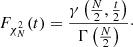
For the P-parametric model, if the quantile of the  statistic is qred, the corresponding significance level is
 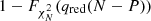 . For example, in the case of a five-parameter model, for 1000 observation points, the
  quantiles equal to 1.00, 1.03 and 1.10 correspond to the significance levels of ∼54%, ∼29%, and ∼2%, respectively. If the number of observation points is 3000, the quantile values 1.00, 1.03 and 1.10 correspond to the significance levels of ∼52%, ∼14%, and ∼0.01%, respectively.
Currently, we have developed an algorithm for calculating the light curve of a transiting star-planet, and its derivatives. It is based on a previously developed algorithm for calculating the intensity decrease due to eclipse and published in Abubekerov & Gostev (2013). The model we use in this algorithm is simplified in comparison with JKTEBOP by neglecting the reflection and gravity darkening effects. Integration is performed using Gaussian quadrature or by expressing the integrals in terms of elliptical integrals. Unlike integration over concentric rings, this approach allows us to obtain a result with a close-to-extended precision, that is, 19 place values. Although the precision of the ultimate result of the light curve calculation is a bit lower (about 18 place values), it is sufficient to exclude any noticeable influence of the non-physical contribution to the residual. We note that there are other algorithms for calculation of the light intensity, for example, Mandel & Agol (2002), Gimenez (2006), and Koch et al. (2010). The advantage of our algorithm over that of Abubekerov & Gostev (2013) is that it works not only for linear and quadratic, but also for square-root, cubic, and logarithmic limb-darkening laws. Furthermore, our algorithm allows the derivatives of the light curve to be calculated with a high precision. The derivative values are useful for implementing fitting methods. Moreover, we then implement analytical fitting under the assumption of linear dependence on limb darkening coefficients. This paper outlines the key points of the algorithm and provides a reference to its current C demo implementation, including an example of fitting. We also test the algorithm by applying it to a well-known observational data set – the transit light curve of the HD 209458 binary from Brown et al. (2001). We analyze how the introduction of the additional limb-darkening law decreases the residual and we compare our results with similar results obtained by Southworth et al. (2007) using JKTEBOP.
2. Calculations
2.1. Light curve calculation
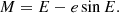
For a star moving in an elliptical orbit with eccentricity e the mean anomaly is related to eccentric anomaly by the Kepler-equation:
 (1)
(1)
Here
 (2)
(2)
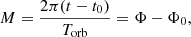
t and Φ is the observation time and phase; t0 and Φ0 are the time and the phase of the periastron passage, and Torb is the orbital period.
If 0 ≤ e < 1, Eq. (1) has unique solution for E, which depends on M and e. We write this solution as a function of two variables E = E(M, e) determined by the condition
 (3)
(3)
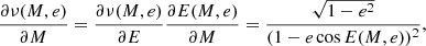
We differentiate Eq. (3) with respect to e and M to obtain the derivatives
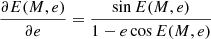 (4)
(4)
and
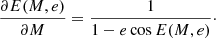 (5)
(5)
The true anomaly ν is related to an eccentric anomaly by the following well-known equation:
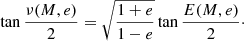 (6)
(6)
The distance between the component centers of the binary star-planet system in elliptical orbit is given by the following formula:
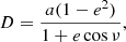 (7)
(7)
where a is the sum of the major axes of the component orbits. The size of the sky-plane projection of the segment between the component centers in the units of a is
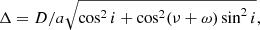 (8)
(8)
where ω is longitude of the periastron and i is the angle between orbital and sky planes (inclination).
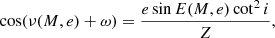
At the moment of an inferior conjunction, that is, at the time when radius-vector of the planet coincides with the perpendicular projection of the line of sight onto the orbital and the star is farther from the Earth than the planet, ν = 3π/2−ω. We note that when the star is farther from Earth than the planet (and hence can be occulted), sin(ν + ω) < 0.
We now express ν from formula Eq. (6) and substitute it into Eq. (7) to obtain

where
 (9)
(9)
To calculate the derivatives of the light curve with respect to M, ω, e, and i, it would be useful to have formulae for derivatives of Δ with respect to these parameters. For this, we first give the formulae
 (10)
(10)
![Mathematical equation: $$ \begin{aligned}&\frac{\partial \nu (M, e)}{\partial e} = \frac{\sqrt{1-e^2} \sin E(M, e)}{1 - e \cos E(M, e)} \left[ \frac{1}{\sqrt{1-e^2}} + \frac{1}{1 - e \cos E(M, e)} \right]. \end{aligned} $$](/articles/aa/full_html/2020/01/aa36731-19/aa36731-19-eq16.gif) (11)
(11)
Below we give the formulae for these derivatives assuming that Υ(M, e, ω, i)≠0, that is, by eliminating the set of quantities M, e, ω, i determined by the condition that i = π/2 and cos(ν(M, e)+ω) = 0. For this set Δ is not analytical. If at least one of the latter two equalities does not hold, using Eqs. (10) and (11) we obtain1:
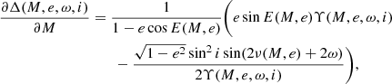 (12)
(12)
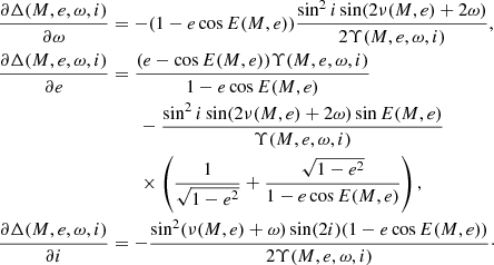
We note that with the smaller e, the weaker the dependence of Δ on ω and Φ0 (see Eq. (2)) at constant Φ0 − ω. At e = 0, Δ does not depend on ω and Φ0 at constant Φ0 − ω. This creates uncertainty in Φ0. At e = 0 the phase (or time) of periastron passage is completely uncertain, as well as ω. Φ0 set the shift of light curve along time and large (or full) uncertainty in Φ0 is not convenient. If we go to variable λ = Φ0 − ω, the dependence of Δ(Φ − λ − ω, e, ω, i) on ω weakens with decreasing e, at e = 0, Δ(λ − ω, 0, ω, i) does not depend on ω. This corresponds to a large uncertainty for the periastron position at small e and a full uncertainty for the periastron position at e = 0. At the same time, dependence on other variable λ persists at e = 0. In such variables, the position of the light curve along the time axis (phase) is not tied to the moment of the passage of the periastron. If we use variables λ and ω instead of Φ0 and ω, it may be necessary to calculate the derivative of Δ(M, e, ω, i), where M = Φ − λ − ω), with respect to ω. This derivative is given by the following formulae
In particular, 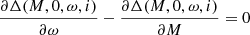 . At small, finite eccentricities of e, the above difference between the derivatives can be much smaller than each of these derivatives itself. Because of this, computing the above difference by direct subtraction introduces significant error due to the machine procedure of rounding off. The following formulae may be useful to obtain the result without such error:
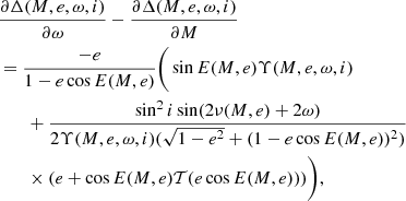 (13)
(13)
where

The formula Eq. (13) obtained by transformation2

After the brackets remove and terms that are 1 cancel in the numerator, all terms are small at small e.
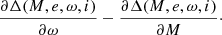
We then calculate the minimum value of Δ in eccentric orbit when the star is farther from Earth than the planet and can be occulted. In the case of i = π/2 and sin(ν + ω) < 0 the minimum value of Δ(M, e, ω, i) is zero and it is achieved at the time of inferior conjunction, i.e., at ω + ν = 3π/2. In general, this minimum is determined from the equation
We note that the left-hand part of the latter equation can be calculated even if Υ(M, e, ω, i) = 0 (then the result is 0). In view of Eq. (12), the latter equation can be written as
 (14)
(14)
where

In the case of i = π/2 the solution of Eq. (14) with respect to M corresponds to the time of inferior conjunction, ν(Mmin, e) = 3π/2−ω, and can be expressed analytically:
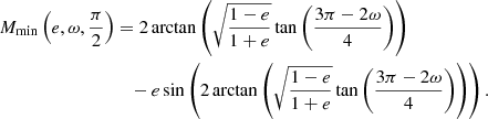 (15)
(15)
At arbitrary 0 < i < π, Mmin(e, ω, i) differs slightly from  and can be calculated by iteratively solving Eq. (14) starting from
  as an initial approximation. It is useful to calculate Mmin(e, ω, i) to set the initial phase to the minimum, that is, to align the calculated and observable minima.
2.2. Minimization by limb-darkening coefficients
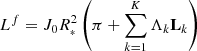
The intensity of the light of the binary system is
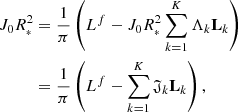
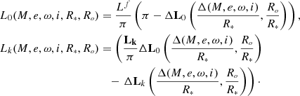
![Mathematical equation: $$ \begin{aligned} L(\Delta , \displaystyle {R}_{\scriptscriptstyle {*}}, \displaystyle {R}_{\scriptscriptstyle {o}}, \boldsymbol{\Lambda })&= J_0 \displaystyle {R}_{\scriptscriptstyle {*}}^2 \Bigg [ \pi - \Delta \mathbf L _{0} \left(\frac{\Delta }{\displaystyle {R}_{\scriptscriptstyle {*}}}, \frac{\displaystyle {R}_{\scriptscriptstyle {o}}}{\displaystyle {R}_{\scriptscriptstyle {*}}} \right) +\nonumber \\&\quad + \sum _{k=1}^K \Lambda _k \left(\mathbf L _{k} - \Delta \mathbf L _{k}\left(\frac{\Delta }{\displaystyle {R}_{\scriptscriptstyle {*}}}, \frac{\displaystyle {R}_{\scriptscriptstyle {o}}}{\displaystyle {R}_{\scriptscriptstyle {*}}} \right) \right) \Bigg ], \end{aligned} $$](/articles/aa/full_html/2020/01/aa36731-19/aa36731-19-eq30.gif) (16)
(16)
when sin(ν + ω) < 0, that is, if the star is farther from Earth than the planet and can be eclipsed. Otherwise 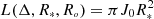 .
.
Here J0 is the brightness at the stellar center; K is the number of the adopted limb-darkening law; R∗ is the stellar radius divided by a and expressed in units of a; Ro is the radius of the planet divided by a; Λk are the limb darkening coefficients; ΔLk are the contributions to the flux decrease; and Lk are the contributions to the out-of-eclipse flux according to the limb-darkening laws used. The algorithm for the calculation of ΔLk, their derivatives, and the formula for Lk for the linear, quadratic, square-root, cubic, and logarithmic limb darkening laws can be found in Abubekerov & Gostev (2013).
In view of the above paper,  , ΔL0 = ΔL0. Depending on the set of limb-darkening coefficients used, Lk may take following values:
  for linear limb-darkening law;
  for quadratic limb darkening law;
  for square-root limb-darkening law;
  for cubic limb-darkening law; and
  for logarithmic limb-darkening law. Respectively, ΔLk may take ΔLl, ΔLq, ΔLQ, ΔLC, ΔLL. The current implementation of this algorithm is referred to as Occultation. Pack3; it contains a code for computing the contributions to the flux decrease according to linear, quadratic, and square-root limb-darkening laws.
We then show how the dependence of the flux on the limb-darkening coefficients can be reduced to some linear dependence. Let Lf be the known full out-of-eclipse intensity of the light of the binary (with appropriate normalization it can be set equal to unity).
Then
 (17)
(17)
or
 (18)
(18)
where
 (19)
(19)
We now express  with Eq. (17), and substitute into Eq. (19) to obtain 𝔍-on-Λ dependence:
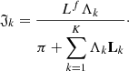
To obtain inverse dependence, we substitute the right part of Eq. (18) into Eq. (19):
 (20)
(20)
In such notation,
 (21)
(21)
where 𝔍 denotes the column (𝔍1…𝔍K)T,
Thus, according to Eq. (21), the flux is linearly dependent on some variable 𝔍, and 𝔍 depends uniquely on limb-darkening coefficients. We can fit the light curve analytically using coefficients 𝔍, and hence the limb-darkening coefficients.
Let the observational data be a set of N triples {Φj, lj, σj}, j = 1…N, where the first quantity is the phase of j-th observation:

where tj is the time of j-th observation; lj, is the intensity at tj, and σj, the uncertainty (standard deviation) of the intensity at tj.
Let t0 be the time of the periastron passage and  be the periastron phase at which the mean anomaly equals zero.
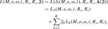
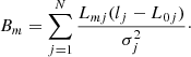
The interpretation problem then reduces the data and finds such Φ0, e, ω, i, R∗, Ro, and 𝔍 that the residual
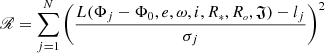 (22)
(22)
reaches its minimum. If lj have a normal distribution, ℛ is distributed as χ2 with N degrees of freedom. The minimum of ℛ is distributed as χ2 with N − P degrees of freedom if minimization performed by P linear parameters. For nonlinear minimization, this statement can be true only by an approximation; see Andrae (2010) for more. For the purposes of this paper, however, we neglect the nonlinearity at the minimum point and consider ℛ/(N − P) as  3.
3.
Given that L has a linear dependence on 𝔍, the values of 𝔍 yielding the minimum of the residual at fixed Φ0, e, ω, i, R∗, Ro can be found analytically. Let  , k = 0…K, j = 1…N. Then
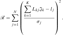 (23)
(23)
Minimizing Eq. (23) with respect to 𝔍 is the standard linear regression problem. The corresponding solution values are  , where
  is the inverse of matrix
  ,
,
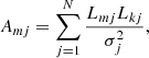
B is a column vector.
Substituting 𝔍fit instead of 𝔍 in Eq. (23) yields the expression for the residual, which is minimized with respect to limb-darkening coefficients and depends on geometric parameters exclusively. The fitted values of Λ can be found using Eq. (20).
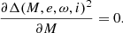
We also note that given that 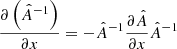 , we can easily calculate the derivative 𝔍fit with respect to each geometric parameter:
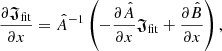
where x is a geometric parameter.
We emphasize that 𝔍fit depends on lj. If we calculate Eq. (22) with 𝔍 = 𝔍fit, ℛ is distributed as χ2 with N − K degrees of freedom.
Next, minimization with respect to geometric parameters can be performed with the any first-level optimization method (for instance, Levenberg–Marquard). We note that during interpretation, in Eq. (22), we can go to variables L(Φj − Φl − ω, e, ω, i, R∗, Ro, 𝔍), where Φl = Φ0 − ω to eliminate correlations between Φ0 and ω at small e. In this case, we use Eq. (13) to calculate the derivatives with respect ω.
3. Interpretation of the light curve HD 209458
Table 1 contain the results of the calculation of parameters with OccultationPack3.
Results of the fitting of the light curve of the binary HD 209458 using OccutationPack3.
Here we analyze the high-precision transit light curve of the exoplanet binary HD 209458 from Brown et al. (2001), which has been used repeatedly to infer reliable values of the geometric parameters of the binary system and the limb-darkening coefficients. This observational material is, therefore, well-suited for debugging and testing the operation of a software package. The observed light curve presented in Brown et al. (2001) was obtained with the Hubble Space Telescope (HST) in April–May 2000. The light curve consists of 556 individual brightness measurements with the rms uncertainties between 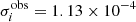 , and
, and 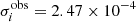 (in units of the out-of-eclipse intensity) in different parts of the light curve. The relative uncertainties (expressed as fractions of the eclipse depth) are between ∼7 × 10⁻³ and ∼1.5 × 10⁻².
In our analysis of the observational data, the fitted parameters were: the radius of the exoplanet rp, the radius of the star rs, the inclination i, the linear (Λl) and quadratic (Λq), and square-root (ΛQ) limb-darkening coefficients. We assumed the orbital period to be 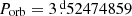 and the sum of the major semi-axes of the orbit to be equal to one. The time of the first minimum is 0.93675 d.
The fit was made according to Newton’s method. We can empirically estimate the accuracy of the result as 12 significant digits for the fitted values. This estimate is based on the differences of the last elements in the iterative sequence of the Newton method.
The uncertainties of the fitted parameters completely coincide with the errors obtained using JKTEBOP in Southworth et al. (2007). Moreover, the discrepancy between the values we obtained obtained and the values obtained in Southworth et al. (2007) are much less than their uncertainties. We note that the values obtained in Gimenez (2006) are not so close to those given above. While the fitted values agree with Southworth et al. (2007) within their uncertainties we have a noticeable difference in residuals  .
.
The analysis of the light curve of HD 209458 in terms of the linear limb-darkening law performed in Southworth et al. (2007) using JKTEBOP package yielded a minimum residual of  corresponding to the maximum significance level of α = 1%. An analysis performed using our algorithm in terms of the linear limb-darkening law yields a minimum residual of
  corresponding to the maximum significance level of α = 2.5%
Our analysis of the light curve of HD 209458 in terms of the quadratic limb-darkening law using OccultationPack yields a minimum residual of  , which corresponds to the maximum significance level of α = 30%. An analysis performed under the same conditions in Southworth et al. (2007) yields a substantially greater residual,
  , corresponding to the maximum significance level of α = 23%.
Our analysis of the light curve of HD 209458 in terms of the square-root limb-darkening law using OccultationPack yields a minimum residual of  , which corresponds to the maximum significance level of α = 31%. A similar analysis performed with JKTEBOP package Southworth et al. (2007) yields a substantially greater residual,
  , corresponding to the maximum significance level of α = 23%.
Thus, more precise computations which exclude the need to account for calculation errors allow us to make better conclusions about the statistically significant decrease in the residual resulting from adding a quadratic term to the limb-darkening law. Moreover, the elimination of non-physical contribution to the residual offers an opportunity of dealing with nonempty confidential set at a higher significance level (lower confidential level).
Additionally, we can conclude that the fit by both the square-root and quadratic limb-darkening coefficients does not result in any noticeable decrease in the residual compared to the case when only one of these limb-darkening laws is used (χ2 = 1.0402, α = 31%).
Also, we realized fit (including the time of the first minimum) in the number of fitted parameters. The fitted time is 0.9367383, 0.9367340, and 0.9367338 for linear, quadratic, and square-root laws, respectively. Significant changes in the value of the residual and other fitted parameters did not occur.
It is worth mentioning that minima of the light curves obtained with modern space telescopes may contain several thousand data points, resulting in even more significant effect of the non-physical contribution to the residual. We note that the analysis presented here does not imply an a priori truth of the limb-darkening model. The possibility of using such a model is considered a hypothesis, the reliability of which is evaluated statistically. In particular, the ability to work with a non-empty confidence set is evaluated here (maximum significance level). It is important to note that we cannot be absolutely sure of the correctness of the model used. In particular, spots and granulation can modify the shape of the transit via changing the limb darkening because they change the stellar intensity profile Csizmadia et al. (2013) and Chiavassa et al. (2017).
4. Numerical testing
For greater certainty in our conclusions we carried out three numerical tests. First of these was modeling the χ2 decrease through the introduction of a limb-darkening law that is more consistent with observations. We generated a synthetic light curve using the values of fitted parameters for HD 209458 and quadratic limb-darkening law. The synthetic observational values was L(tk, x)+ξk, where tk is a time of kth observation, x is a set of values of parameters, L(tk, x) is the corresponding light curve value, ξk is a normally distributed random number with standard deviation  that is k level of uncertainty for light curve HD 209458 from Brown et al. (2001). A quadratic limb-darkening model played a role of an “ideal model” for such synthetic observational data. We can say that
  for linear limb-darkening was about 0.1 greater than that of
  for quadratic limb darkening. It matches a
  decrease for the real light curve. The same effect also occurs if we proportionally reduce the standard deviation of ξk.
Second, we made artificial distortion in calculation of the light curve by adding 0.0015(1 − L(tk, x))ϵk to the values of the light curve, where ϵk = 1 if k is even and -1 if odd. We recall that the maximal light decrease 1 − L(tk, x) is about 0.015, so term (1 − L(tk, x))ϵk is distroted by the 5th to 6th decimal place in L(tk, x). Then the  (JKTEBOP result 1.056), R∗ = 0.113827, Ro = 0.013764, i = 86.67684, Λl = 0.294, and Λq = 0.345. Thus, calculating the light curve with artificial calculation error, we get result similar to the result of using the JKTEBOP, which leads to a significant increase for
  and no significant shift in fitted values.
Third, we checked whether the increased value of the residual is not attributable to the lack of a minimization procedure for JKTEBOP. We calculated χ2 using the fitted values from Southworth et al. (2007) for quadratic limb-darkening law. We did not find any significant increase in  (its value was 1.04036). Thus, we can conclude that the overestimated value of
  from Southworth et al. (2007) is not caused by the lack of a minimization procedure for JKTEBOP. Hence, errors in the light curve calculation may do not lead to a significant shift of fitted values but at the same time, they lead to a significant increase in
  .
.
We note that if we calculate  with fitted values from Gimenez (2006), we get
  , that is, in this case, there is a significant shift in the fitted parameters.
5. Discussions and conclusions
The above results clearly demonstrate that high-precision algorithms have to be used when computing the light curves to test the hypothesis of whether observational data agrees with theory. The algorithm that we developed is based on Gaussian quadratures and allows computations to be performed with current machine precision. Such precision for the light curve calculation allows for more reliable conclusions about the compatibility of the observed light curve with the adopted model.
In the Occultation.Pack3 algorithm, integration over overlapping disks is performed analytically using either elliptic integrals (there is an efficient algorithm for calculating them with required precision) or Gaussian quadratures after some analytical transformation of the integrand.
The prime advantage of the improved precision of the light curve calculation is that it allows us to make a better assessment of the compatibility of the observed light curve with the adopted model. Because of the elimination of the non-physical contribution to the residual we can draw more reliable conclusions about how significant the variation is for the χ2 in certain cases. For example, we can see how significant the variation of the minimal value is for the residual due to the addition of extra parameters to the fit, including the dependence of the minimal residual on the adopted limb-darkening laws.
We also note that the improvement in the precision of the light curve calculation may have a considerable effect on the minimum residual value even if it translates into no significant changes in the inferred parameter values. Under such circumstances, we can conclude that in practice, JKTEBOP allows for satisfactory results to be obtained in certain cases, such as the determination of the system parameter values within their uncertainties estimated via the Monte-Carlo method (assuming that the model is compatible with observational data). The residuals have to be calculated with higher precision if the interpretation involves no such assumption (in the case that the confidence set turns out to be empty or that statistically significant changes in the residual are in question).
In practice, the algorithm that we developed excludes any non-physical contribution to the residual due to computational errors and it allows us to make more reliable conclusions about the significance of the variation of the residuals in certain cases. For instance, we can get an understanding of how significant the variation of the minimum residual value is by adding extra parameters to the fit. In addition, the opportunity of working at a higher significance level is of value in itself.
Thus, the improvement in the precision of the light-curve computation, in particular, the resulting elimination the non-physical contribution to the discrepancy, allows for a more reliable investigation of the compatibility of the observed light curve with the adopted model.
Our algorithm will make it possible to better analyze the rich observational material supplied by space telescopes. The implementation of the algorithm is publicly available. Currently, we present the code for calculating Δ(M, e, ω, i) and its derivatives, Mmin(e, ω, i), and the dependence of normalized light on geometric parameters computed in terms of linear, quadratic, and square-root limb-darkening laws. The combined code and data files are distributed under the name of Occultation.Pack3.
We also present Demo.Pack which contains a code for calculating the light curve over the given time interval (specified in the parameter file) and the residual  minimized with respect to the limb-darkening coefficients at fixed geometric parameters, as well as the HD 209458 example described above. Occultation.Pack3 and Demo.Pack are available online4.
The following relationships may be useful here: sin 2x = 2 sin x cos x, cos x2 = (1 + cos 2x)/2, sin x2 = (1 − cos 2x)/2.
Here we use formulae  .
.
To avoid confusion between the concepts of value and distribution of the residual, also taking into account Andrae (2010), we denote the residual as ℛ, not χ2.
Acknowledgments
We thank Professor Anatoly Cherepashchuk for the helpful suggestions and useful comments that improved the presentation of the paper.
References
- Abubekerov, M. K., & Gostev, N. Yu. 2013, MNRAS, 432, 2216 [NASA ADS] [CrossRef] [Google Scholar]
- Abubekerov, M. K., & Gostev, N. Yu. 2016, MNRAS, 459, 2078 [NASA ADS] [CrossRef] [Google Scholar]
- Andrae, R. 2010, ArXiv e-prints [arXiv:1012.3754v1] [Google Scholar]
- Brown, T. M., Charbonneau, D., Gilliland, R. L., Noyes, R. W., & Burrows, A. 2001, ApJ, 552, 699 [NASA ADS] [CrossRef] [Google Scholar]
- Chiavassa, A., Caldas, A., Selsis, F., et al. 2017, A&A., 597, 94 [Google Scholar]
- Csizmadia, S., Pasternacki, T., Dreyer, C., et al. 2013, A&A, 549, 9 [Google Scholar]
- Gimenez, A. 2006, A&A, 450, 1237 [Google Scholar]
- Hellard, H., Csizmadia, S., Padovan, S., et al. 2019, ApJ, 878, 119 [NASA ADS] [CrossRef] [Google Scholar]
- Knutson, H. A., Charbonneau, D., Noyes, R. W., Brown, T. M., & Gilliland, R. L. 2007, ApJ, 655, 564 [NASA ADS] [CrossRef] [Google Scholar]
- Koch, D. G., Borucki, W. J., Rowe, J. F., et al. 2010, ApJ, 713, 131 [NASA ADS] [CrossRef] [Google Scholar]
- Mandel, K., & Agol, E. 2002, ApJ, 580, L171 [NASA ADS] [CrossRef] [Google Scholar]
- Nelson, B., & Davis, W. 1972, ApJ, 174, 617 [NASA ADS] [CrossRef] [Google Scholar]
- Popper, D. M., & Etzel, P. B. 1981, AJ, 86, 102 [NASA ADS] [CrossRef] [Google Scholar]
- Southworth, J. 2008, MNRAS, 386, 1644 [NASA ADS] [CrossRef] [Google Scholar]
- Southworth, J., Maxted, P. F. L., & Smalley, B. 2004, MNRAS, 351, 1277 [NASA ADS] [CrossRef] [Google Scholar]
- Southworth, J., Wheatley, P. J., & Sams, G. 2007, ApJ, 379, L11 [Google Scholar]
All Tables
Results of the fitting of the light curve of the binary HD 209458 using OccutationPack3.
Current usage metrics show cumulative count of Article Views (full-text article views including HTML views, PDF and ePub downloads, according to the available data) and Abstracts Views on Vision4Press platform.
Data correspond to usage on the plateform after 2015. The current usage metrics is available 48-96 hours after online publication and is updated daily on week days.
Initial download of the metrics may take a while.