© ESO 2019

1. Introduction

The minimum orbital intersection distance (MOID) at a given epoch between two objects orbiting a common primary is the distance between the closest points of their osculating orbits. The problem of computing the MOID is as old as Kepler’s laws. However, the need for a quick and accurate solution has increased as its role in several branches of Celestial Mechanics and Astrodynamics has become more and more prominent. Nowadays, the MOID is used primarily to provisionally discard objects from large space debris catalogs when collisions with a given target can be excluded (Hoots et al. 1984; Woodburn et al. 2009; Casanova et al. 2014), and to predict possible close encounters of asteroids and comets with the planets (mainly, Earth and Mars for the asteroids, and Jupiter for the comets) prior to the study of their dynamics (Milani et al. 1989, 2000; Harris & Bailey 1998; Wlodarczyk 2013). Regarding the space debris problem, according to Gorno (2019), “the ever-growing population of space debris (or space junk), especially in the LEO zone, is posing serious issues to the survival of man-made objects in space. Every mission planner has to take into account the possibility of the satellite colliding with relatively small pieces of debris, which, traveling at orbital speeds, could jeopardize the survival of the mission”. The Center for Space Standards and Innovation (CSSI) offers the Satellite Orbital Conjunction Reports Assessing Threatening Encounters in Space (SOCRATES) service (Kelso & Alfano 2006), intended to help satellite operators avoid undesired close approaches through advanced mission planning. According to Kelso & Alfano (2006), “hundreds of conjunctions within one kilometer occur every week, with little or no intervention, putting billions of dollars of space hardware at risk, along with their associated missions”. As for the close planetary encounters, the MOID between the asteroid and Earth turns out to be one of the most important parameters when assessing the impact risk (Sitarski 1968).

The calculation of the MOID involves two Keplerian orbits, represented by their classical orbital elements. The orbital elements change over time as a result of perturbations. In the case of the asteroids, for example, Sekhar et al. (2016) show that Einstein’s General Theory of Relativity predicts a significant orbital precession if the object has both a moderately low perihelion and a small semimajor axis, and observe that the effect “could play an important role in the calculations pertaining to MOID and close-encounter scenarios in the case of certain small solar system bodies (depending on their initial orbital elements)”. Due to the time evolution of the orbital elements, the MOID itself is a function of time. Thus, understanding the evolution of the MOID over long time frames is important for impact risk assessment. In the case of asteroids, such MOID monitoring makes it possible to better assess the risk of a possible impact with Earth. Recently, Monte Carlo methods have been implemented to calculate the impact probability of an asteroid with Earth (Rickman et al. 2014).

The orbit of an asteroid is known with an uncertainty that depends on the quality of the observations and that reflects in the uncertainty of the MOID. For its assessment, the covariance matrix must be propagated, with the inherent requirement to explicitly compute the derivatives of the MOID with respect to some variables. Bonanno (2000) uses an approximate analytical expression to obtain the required partial derivatives of the MOID. Alternatively, the differentiation can be carried out numerically, in which case, it is beneficial to employ fast, accurate, and safe algorithms to calculate the MOID without increasing the uncertainty brought by the observational data. In this respect, it is worth remembering that a singularity appears in the computation of the uncertainty of the MOID in the orbit-crossing case. This problem was studied and solved by Gronchi & Tommei (2007).

Using models currently accepted for the long-term dynamical evolution of the Solar System, the MOID computation makes it possible to determine the cometary impact rates on the Moon and on the terrestrial planets during the late heavy bombardment (Rickman et al. 2017). Fast MOID computation is in high consideration and demand also to facilitate the analysis of large catalogs of objects. Obviously, accuracy is also a key issue. Here, the latter is meant to encompass both precision (low random errors) and trueness (low systematic errors) (ISO Central Secretary 1994).

In summary, a fast and accurate MOID computation method is an asset in several common problems. Many methods for computing the MOID have been published in the literature over the past seven decades. The majority are approximate numerical methods (Sitarski 1968; Dybczinski et al. 1986). However, more recently, algebraic (Kholshevnikov & Vassiliev 1999; Gronchi 2005) and analytical (Bonanno 2000; Armellin et al. 2010) approaches have been established, and some hybrid methods have appeared (see, e.g., Derevyanka 2014).

The Space Dynamics Group (SDG) of the Technical University of Madrid developed a fast and accurate numerical method for the computation of the MOID. This method is called SDG-MOID (Hedo et al. 2018) and is based on two algorithms. Algorithm 1 determines the distance between a point and an ellipse in three-dimensional space by composing two orthogonal distances: the distance from the point to its orthogonal projection onto the plane of the ellipse and the distance from the ellipse to the projected point. The former is trivial to determine, whereas the latter (which, for the sake of brevity, will be referred to as the in-plane distance) can be obtained in closed form with elementary functions only under specific circumstances¹, the general scenario requiring application of an iterative method to the solution (as accurate as desired) of a transcendental equation. Algorithm 2 calculates the minimum distance between two confocal ellipses in the following way: one of the two ellipses is discretized in a finite set of points by means of a uniform partition of the interval [0, 2π], where its eccentric anomaly is defined – see Eqs. (3) and (4) below– and the corresponding distances to the other ellipse are computed by means of Algorithm 1: this yields a discrete function approximation of the distance. Then, the partition intervals containing the local minima of the distance are identified, the distance function in these intervals is minimized using the golden-section search, and the minimum minimorum is selected.

This work considers asymptotic expansions for the computation of the in-plane distance component in Algorithm 1 of the SDG-MOID method. These asymptotic procedures are tested to assess the gain in computing speed, the corresponding accuracy loss, and hence the benefits of their introduction: they are worth adopting if a positive balance between advantages and disadvantages is achieved. Our tests employed the NEODyS (Near Earth Object – Dynamics Site) catalog (NEODyS Consortium 2011) for MJD 58600 to compute the position uncertainty and the Earth MOID of NEOs (Near Earth Objects). Improvements of Algorithm 2 are also being undertaken: the aim is to preserve accuracy by decreasing the resolution of the discretization, and by limiting it to the vicinity of the minimum minimorum. However, these enhancements are under development and out of the scope of this contribution.

The paper is structured as follows. Section 2 features an illustration of the mathematical foundations of the two asymptotic expansions, here proposed as approximate procedures to compute the in-plane distance component. These methods constitute one-parameter families of procedures, the parameter being the number of terms retained in the expansions. Section 3 gives an assessment of the minimum MOID accuracy (trueness) needed in order not to deteriorate the total uncertainty of the starting orbital data. Section 4 presents the results of the accuracy and computing speed tests on the two families of asymptotic expansions and compares them with the performance of the exact in-plane distance determination carried out with SDG-MOID. The family exhibiting the best performance was tested for accuracy and computing speed on the Earth MOID of NEOs, and the results were compared with the SDG-MOID determinations. Section 5 features the benefits that the asymptotic expansions can bring when applied to the time monitoring of the MOID through the presentation of an application to the space debris problem. The paper closes (Sect. 6) with a summary and a discussion of the relevance of the results.

2. Mathematical foundations

This section summarizes the theory of asymptotic expansions in powers of a small parameter. It describes in detail the application of two such methods to the determination of the in-plane distance component.

2.1. Asymptotic expansions in powers of a small parameter

Given the function f : ℝ^n + 1 ↦ ℝ, and

$$\begin{array}{c}\hfill z=f(x;y_1,y_2,\dots ,y_n),\end{array}$$(1)

with x ∈ ℝ : x ≪ 1 the independent variable, z ∈ ℝ the dependent variable, and y_k ∈ ℝ (k = 1, 2, …, n) a set of parameters, the asymptotic expansion of z in powers of x is defined as:

$$\begin{array}{c}\hfill z\sim {\displaystyle \sum _{i=0}^N{c}_i(y_1,y_2,\dots ,y_n)x^i,}\end{array}$$(2)

where N is the order of the expansion, meaning, the highest power of x among the terms that appear in the expansion, and c_i ∼ O(1) (i = 0, 1, 2, …, N) are the functional coefficients. N is used to control the accuracy of the asymptotic expansion. The advantages of the truncation of the expanded function are a higher speed of the computation of the approximate function compared with the original function, and a more treatable mathematical expression for algebraic manipulation and computation. The main drawback consists of the introduction of truncation errors, meaning, the expansion only provides an approximation to true values. The smaller the value of x and the higher the value of N, the better the approximation of z obtained from the corresponding truncation. The procedure is useful if the improvement in computing speed compensates for the inherent loss of accuracy.

Several choices for the asymptotic expansion exist. In this paper, we consider the two most suitable options, meaning, an expansion in the critical eccentric anomaly, and an expansion in the minimum distance. They are described here below.

2.2. Expansion in the critical eccentric anomaly

Let 𝔢 be an ellipse in the standard Cartesian parametric representation relative to its symmetry axes:

$$\begin{array}{cc}\hfill x(u)& =acos(u),\hfill \end{array}$$(3)

$$\begin{array}{cc}\hfill y(u)& =\sqrt{1-e^2}asin(u),\hfill \end{array}$$(4)

where u is the eccentric anomaly, a is the semi-major axis, and e ≪ 1 is the eccentricity. Let P be a coplanar point with Cartesian coordinates (α, β) in the previous axes. Find the eccentric anomaly u_* that minimizes the distance d(P, E):E ∈ 𝔢, defined as

$$\begin{array}{c}\hfill d(u;a,e,\alpha ,\beta )=\sqrt{{(\alpha -x(u))}^2+{(\beta -y(u))}^2}.\end{array}$$(5)

This problem was addressed as part of the presentation of the SDG-MOID method (Hedo et al. 2018). The main conclusions of that study can be summarized as follows:

1. d(u) is 2π-periodic, and, therefore, it has an even number of extreme points. All global maxima and minima are always critical points.

2. The critical points u^* of Eq. (5) (equivalent to the critical points of its square) must satisfy the transcendental equation

   $$\begin{array}{cc}\hfill f(u;a,e,\alpha ,\beta )& =a\alpha sin\left(u\right)-\sqrt{1-e^2}a\beta cos\left(u\right)\hfill \\ \hfill & -e^2{a}^{2}sin\left(u\right)cos\left(u\right)=0.\hfill \end{array}$$(6)

   Equation (6) admits a minimum of two and a maximum of four solutions in the interval [0, 2π) (including, in the latter case, a possible double root resulting from the coincidence between one maximum and one minimum). Solving Eq. (6) is equivalent to solving a polynomial equation of degree four. The latter admits exact solutions, but, as pointed out in Hedo et al. (2018), the loss of precision due to the rounding errors may change their character, for example, from real to complex. Since the interest is in real solutions, this approach cannot be employed.

3. The minima must also satisfy the condition

   $$\begin{array}{c}\hfill f^{\prime }(u)>0.\end{array}$$(7)

   The geometric study showed that the absolute minimum (and the absolute maximum) always exists. Let ℳ = {u_i, i = 1, 2, …, m} be the set of eccentric anomalies corresponding to the minima (they satisfy Eqs. (6) and (7)). Then,

4. the eccentric anomaly u_* yielding the minimum distance in ℳ is

   $$\begin{array}{c}\hfill u_{\ast }=\{u_i\in \mathcal{M}:d(u_i)\le d(u_j),\forall j\ne i\}.\end{array}$$(8)

   The symbol ≤ takes into account the case in which multiple u_*s are associated with the same minimum distance.

The results can be summarized as follows:

• If e = 0 (circular orbit), the solution is simply u_* = arctan(β/α).

• If e >  0 and α = 0 or β = 0 (P on a symmetry axis of 𝔢), closed-form solutions for u_* always exist.

• If e >  0, α ≠ 0 and β ≠ 0, numerical techniques constitute the only method to solve the equation, with the additional requirement that u_* be in the same quadrant as P. In particular, iterative methods offer the best results (i.e., the fastest and the most accurate), and a suitable seed for such numerical approximations is u₀ = arctan(β/α).

Equation (6) defines an implicit function u_*(a, e, α, β); and, when e ≪ 1, a truncated series expansion in powers of e is convenient:

$$\begin{array}{c}\hfill u_{\ast }^{(N)}(a,e,\alpha ,\beta )={\displaystyle \sum _{i=0}^N{c}_i(a,\alpha ,\beta )e^i.}\end{array}$$(9)

The parameter N ∈ ℕ controls the finite number of terms in the truncated series, whereas the c_i(a, α, β) coefficients must be computed to approximate the critical eccentric anomaly.

Substituting u_* as given by Eq. (9) into Eq. (6) yields the expansion in powers of e. Since $f=\sum _{i=0}^N{f}_i{e}^i$ must satisfy Eq. (6), the c_i’s can be calculated by successive cancellation of the f_i’s in increasing order. This problem was solved for N up to 6 using the MAPLE 2017.3 math software. The result is:

$$\begin{array}{cc}& c_i=0\mathrm{if}i\mathrm{is}\mathrm{odd},\hfill \end{array}$$(10)

$$\begin{array}{cc}& c_0=arctan\left(\frac{\beta }{\alpha }\right)(\mathrm{case}e=0\mathrm{above}),\hfill \end{array}$$(11)

$$\begin{array}{cc}& c_2=\alpha \beta (\frac{a}{{({\alpha }^2+{\beta }^2)}^{3/2}}-\frac{1}{2({\alpha }^2+{\beta }^2)})\hfill \end{array}$$(12)

$$\begin{array}{cc}& c_4=-\frac{\alpha \beta (-8a^2{\alpha }^2+8a^2{\beta }^2+{\alpha }^4+4{\alpha }^2{\beta }^2+3{\beta }^4)}{8{({\alpha }^2+{\beta }^2)}^3}\hfill \\ \hfill & +\frac{a\alpha \beta ({\beta }^2-\frac{1}{2}{\alpha }^2)}{{({\alpha }^2+{\beta }^2)}^{5/2}},\hfill \end{array}$$(13)

$$\begin{array}{cc}& c_6=\frac{\alpha \beta }{{({\alpha }^2+{\beta }^2)}^4}[-\frac{{\alpha }^6}{16}-{\alpha }^4(\frac{a^2}{2}+\frac{13{\beta }^2}{48})\hfill \\ \hfill & +{\alpha }^2(4a^2{\beta }^2-\frac{25{\beta }^4}{48})-\frac{3}{2}{a}^2{\beta }^4-\frac{5{\beta }^6}{16}]\hfill \\ \hfill & +\frac{a\alpha \beta }{{({\alpha }^2+{\beta }^2)}^{9/2}}[-\frac{{\alpha }^6}{8}+{\alpha }^4(a^2-\frac{9{\beta }^2}{8})\hfill \\ \hfill & -\frac{23a^2{\alpha }^2{\beta }^2}{6}+a^2{\beta }^4+{\beta }^6].\hfill \end{array}$$(14)

After substituting Eqs. (10)–(14) into Eq. (9), the Euclidean distance function (Eq. (5)) with $u=u_{*}^{(N)}$ yields the following parametric family of procedures for the approximate computation of the minimum distance:

$$\begin{array}{c}\hfill d_{\ast }^{(N)}(a,e,\alpha ,\beta )=d(u_{\ast }^{(N)}(a,e,\alpha ,\beta );a,e,\alpha ,\beta ),\end{array}$$(15)

in which N = 0, 2, 4, 6 is the parameter. The selection of N is a trade-off between efficiency and accuracy: the lower its value, the more mathematically treatable the final expression contained in Eq. (5), but the lower the accuracy of the resulting distance approximation.

2.3. Minimum distance expansion

Following (Hedo et al. 2018), an alternative approach to the computation of the critical points of the distance function consists of solving the following system of two algebraic equations:

$$\begin{array}{cc}& {\displaystyle \frac{x^2}{a^2}}+{\displaystyle \frac{y^2}{a^2(1-e^2)}}=1,\hfill \end{array}$$(16)

$$\begin{array}{cc}& a^2{e}^{2}xy-\alpha a^{2}y+\beta a^2(1-e^2)x=0.\hfill \end{array}$$(17)

If e = 0, the solution corresponding to the minimum distance is trivial:

$$\begin{array}{cc}& x_0(a,\alpha ,\beta )=\frac{a\alpha }{\sqrt{{\alpha }^2+{\beta }^2}},\hfill \end{array}$$(18)

$$\begin{array}{cc}& y_0(a,\alpha ,\beta )=\frac{a\beta }{\sqrt{{\alpha }^2+{\beta }^2}}·\hfill \end{array}$$(19)

If 0 <  e ≪ 1, let us consider the following decomposition:

$$\begin{array}{cc}& x_{\ast }=x_0+\xi :\xi \sim O(e),\hfill \end{array}$$(20)

$$\begin{array}{cc}& y_{\ast }=y_0+\eta :\eta \sim O(e).\hfill \end{array}$$(21)

Substituting Eqs. (20) and (21) with Eqs. (18) and (19) into Eqs. (16) and (17) leads to a system of two equations to be solved with respect to ξ and η:

$$\begin{array}{cc}& \xi =\xi (a,e,\alpha ,\beta ),\hfill \end{array}$$(22)

$$\begin{array}{cc}& \eta =\eta (a,e,\alpha ,\beta ).\hfill \end{array}$$(23)

Hence, the square of the distance function (Eq. (5)) can be written as:

$$\begin{array}{c}\hfill d^2={(\alpha -x_0-\xi )}^2+{(\beta -y_0-\eta )}^2=d^2(a,e,\alpha ,\beta ).\end{array}$$(24)

A truncated series expansion in powers of e of this function² is

$$\begin{array}{c}\hfill d_{\ast }^{2(N)}(a,e,\alpha ,\beta )={\displaystyle \sum _{i=0}^N{d}_i(a,\alpha ,\beta )e^i,}\end{array}$$(25)

in which the d_i(a, α, β) coefficients need to be specified. In this contribution, the d_i(a, α, β)s were computed for N up to six using the MAPLE 2017.3 math software:

$$\begin{array}{cc}\hfill d_i& =0\mathrm{if}i\mathrm{is}\mathrm{odd},\hfill \end{array}$$(26)

$$\begin{array}{cc}\hfill d_0& ={(\sqrt{{\alpha }^2+{\beta }^2}-a)}^2,\hfill \end{array}$$(27)

$$\begin{array}{cc}\hfill d_2& =\frac{a{\beta }^2(\sqrt{{\alpha }^2+{\beta }^2}-a)}{{\alpha }^2+{\beta }^2},\hfill \end{array}$$(28)

$$\begin{array}{cc}\hfill d_4& =\frac{{a\beta }^2}{4{({\alpha }^2+{\beta }^2)}^{5/2}}(4a{\alpha }^2\sqrt{{\alpha }^2+{\beta }^2}\hfill \\ \hfill & -4a^2{\alpha }^2+{\alpha }^2{\beta }^2+{\beta }^4),\hfill \end{array}$$(29)

$$\begin{array}{cc}\hfill d_6& =\frac{a^2{\alpha }^2{\beta }^2[{\alpha }^2({\beta }^2-a^2)+a^2{\beta }^2+{\beta }^4]}{{({\alpha }^2+{\beta }^2)}^4}\hfill \\ \hfill & -\frac{3a{\beta }^2[-\frac{2}{3}{a}^2{\alpha }^4+{\alpha }^2(a^2{\beta }^2-\frac{{\beta }^4}{12})-\frac{{\beta }^6}{12}]}{2{({\alpha }^2+{\beta }^2)}^{7/2}}·\hfill \end{array}$$(30)

The distance approximation can then be computed by substituting the required number of terms up to N = 0, 2, 4, 6 in Eq. (25). Again, the lower the order N, the more mathematically treatable the final expression (Eq. (24)), and the lower the accuracy obtained for the distance.

3. Accuracy assessment

The original SDG-MOID method introduces negligible errors in the distance computation, meaning, it does not increase the uncertainty of the original orbital data. For an approximate MOID, like the one provided by the methods presented here, the accuracy should not be lower than the minimum uncertainty of the data, the best performance in terms of computing speed being achieved when the former is close to the latter.

The uncertainty of the state vector is usually expressed by its six-dimensional confidence ellipsoid. However, since only the position accuracy is relevant here, we limited our attention to the corresponding three-dimensional confidence (or uncertainty) ellipsoid. Its major axis is aligned very closely with the velocity vector (its direction is tangent to the trajectory), whereas the other two axes define the plane that is normal to the orbit.

The proposed methods were tested on the computation of the Earth MOIDs of Near Earth Objects. In this case, Earth is the primary object, and its orbital eccentricity constitutes the small parameter. Since the Earth’s position vector is known with the highest possible precision (Gronchi et al. 2006), the uncertainty of the MOID is entirely determined by the uncertainty of the orbit of the NEO, expressed by its covariance matrix (Milani et al. 1989).

The space objects of interest are tracked by dedicated observatories, and their data are systematically computed and recorded in catalogs. Each entry has an associated uncertainty (affecting both position and velocity) due to several factors, such as instrument precision, shortage of measurements, truncations, round-off errors (Gronchi et al. 2006). The orbit determination of NEOs is carried out through either radar tracking or optical observations. The former technique is characterized by low measurement errors, but it is applicable to a limited number of objects. The majority of NEOs are monitored by optical observations, which are affected by larger errors owing to the more limited visibility conditions. The NEOs whose orbits are determined by radio telescopes are associated with the smallest position uncertainties, at the level of 100 m, whereas optical determinations are affected by much larger (by at least two orders of magnitude) position uncertainties.

The minimum accuracy required by the approximate algorithm must be greater than the smallest uncertainty in the position vector. Therefore, the smallest error in length (maximum tolerance) is the size of the shortest semiaxis of the 1σ position’s confidence ellipsoids obtained for the subset of NEOs observed with radar tracking. These values were calculated from the covariance matrix data in equinoctial elements of the first 281 radar-tracked Near Earth Asteroids (NEAs)³ of the NEODyS catalogue using the algorithm illustrated in Appendix A. The results are the lengths of the three semiaxes of each 1σ position’s confidence ellipsoid. On the other hand, the geometric mean of the two smallest semiaxes is the radius of a circle whose area is equal to that of the section (ellipse) of the ellipsoid with the plane containing the two shortest axes. This holds because the minimum distance line is in this plane, but its exact orientation is a priori not known. It should be noted that the longest axis – corresponding to the maximum uncertainty due to instability in the sense of Lyapunov – is tangent to the orbit, whereas the MOID always corresponds to a line that is normal to both orbits.

Table 1 is a statistical summary of the data. The several rows contain the minimum, the average, and the maximum values of the sets formed by the three semiaxis lengths (i.e., shortest, intermediate, and longest) of the position’s confidence ellipsoids, and by the geometric mean of the shortest and intermediate semiaxes.

The minimum of the shortest is 6.711 × 10⁻¹⁰ au (∼100 m). Therefore, Δl = 6.711 × 10⁻¹⁰ au is the tolerance to be used to assess the level of trueness for the approximate computation of the Earth MOIDs of all the objects of the NEODyS database:

$$\begin{array}{c}\hfill \mathrm{\Delta }\mathrm{MOID}=|{\mathrm{MOID}}_{\mathrm{true}}-{\mathrm{MOID}}_{\mathrm{approx}.}|\le \mathrm{\Delta }l.\end{array}$$(31)

4. Tests

4.1. Approximate computation of the in-plane distance for low-eccentricity ellipses

The two families of procedures proposed here for the computation of the distance between a low-eccentricity ellipse and a coplanar point, meaning, $d(u_{*}^{(N)})$ (Eq. (15)) and $\sqrt{d_{\ast }^{2(N)}}$ (Eq. (25)), respectively, were coded and tested. Simulations were run on an Intel^® Core^™ I7-8750H at 2.2 GHz processor with 32 MiB of RAM. Accuracy and computing speed tests were executed on an ellipse with unit semimajor axis (a = 1) and eccentricity close to that of Earth’s orbit (e = 1.671022 × 10⁻²), and a set of 616 points evenly distributed in the first quadrant and belonging to a family of concentric circles with radii respectively larger, equal to and smaller than the semimajor axis of the ellipse. The center of the circles coincides with the center of the ellipse. The points form a grid with polar coordinates $(\rho ,\theta ):\rho =\{2^{i-5},i=0,1,\dots ,10\},\theta =\{\frac{j\pi }{110},j=0,1,\dots ,55\}$.

4.1.1. Numerical errors

Table 2 gives a summary of the basic statistical properties, meaning, the minimum, the average, and the maximum value, of the absolute error of the in-plane distances from the selected elliptical orbit to each of the 616 test points (see text). The in-plane distances were obtained with the two families of approximate algorithms at different expansion orders. We observe that the $d(u_{*}^{(N)})$ algorithm is far more accurate than $\sqrt{d_{\ast }^{2(N)}}$ at the same N. With only two terms, it introduces no appreciable error; the $\sqrt{d_{\ast }^{2(N)}}$ algorithm requires four terms to reach a comparable performance.

4.1.2. Execution speed

Table 3 features results and statistics regarding the execution times for the test cases described above. We observe that the two approximate methods are at least ten times faster than the exact distance determination, there are no appreciable differences in execution time between the two approximate algorithms (neither by family nor by number of terms), and the computing speed is inversely proportional to the expansion order.

4.2. Approximate computation of the MOID for low-eccentricity ellipses

The $d(u_{*}^{(N)})$ algorithms exhibit similar execution times but better accuracy than the $\sqrt{d_{\ast }^{2(N)}}$ methods. For this reason, the former one-parameter family, with the expansion order as the parameter, is the method of choice to replace the exact in-plane distance computation method in SDG-MOID. Tests were performed to assess accuracy and execution speed of this method relative to the exact SGD-MOID determination. The simulations consist of the computation of the Earth MOID of objects belonging to the NEODyS database.

4.2.1. Numerical errors for the approximate SDG-MOID

Table 4 reports the most significant statistical properties of the results of the accuracy tests, meaning, the minimum, the average, and the maximum absolute error of the MOID computed using the $d(u_{*}^{(N)})$ algorithm at different expansion orders. The high accuracy (trueness) obtained with N = 2 is the most remarkable outcome.

4.2.2. Execution speed for the approximate SDG-MOID

Table 5 shows the average execution times per distance computation resulting from several determinations – both exact and approximate – of Earth MOID of NEODyS objects, as well as some descriptive statistics and relevant ratios. On average, the $d(u_{*}^{(N)})$ algorithm with N = 2 is 40% faster than the exact SDG-MOID. This result constitutes a remarkable enhancement.

5. Application: time monitoring of the MOID

The first application of the algorithms described in this paper was within a numerical tool called DROMOID (Gorno 2019) that monitors the MOID of two LEO objects (e.g., a satellite and a space debris object) over time. DROMOID implements the DROMO orbital propagator (Urrutxua et al. 2016)⁴ and the SDG-MOID algorithm. The evolution of the two orbits over a selected time period and at a given sampling resolution was computed using DROMO. Then, the osculating classical orbital elements of the two objects were obtained at each sampling time and used to determine the evolution of the MOID. One of the advantages of the tool is that in input it accepts the space debris ephemerides of NASA’s Two-Line-Element (TLE) database, which are always accessible and are considered the most reliable public source of orbital data. The time performance of DROMOID depends on the time resolution. However, the 2-weeks propagation of 19 664 valid TLE ephemerides at a sampling resolution of 1 h takes only 9.5 h on an I5 processor. DROMOID can efficiently predict close encounters, as shown by the following example, for the detailed analysis of which the reader is referred to Gorno (2019). According to SOCRATES, the Space Technology EXperiments (STEX) satellite and a debris from the CBERS 1 satellite had a close approach with a minimum range of 0.638 km on June 21st 2019 at 18:57:58.129 UTC.

The two orbits were propagated with DROMOID over a period of seven days starting at noon on June 16 2019 (58 650.5 MJD) and using a sampling interval of one minute. The resulting MOID is smaller than three kilometers during the whole propagation period, and it oscillates very rapidly between zero and three kilometers, the amplitude of the variations getting smaller (below two kilometers) approximately between day two and day six, and the oscillations reaching the highest frequency between day five and day six (see Fig. 1). When the MOID is zero, the two orbits are crossing each other, but this does not necessarily correspond to a collision, because the latter requires time coincidence⁵. Hence, SDG-MOID can be reliably employed as part of the first processing stage of a more complex tool for the real-time monitoring of thousands of space debris in the determination of the risk of collision with a spacecraft.

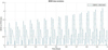Fig. 1. MOID between STEX and CBERS 1 between day five and day six after 12 p.m. on June 16 2019 (58650.5 MJD). Simulations made with DROMOID.

6. Conclusions

Two families of algorithms for the approximate computation of the distance from an ellipse to a coplanar point are proposed for the case of low-eccentricity ellipses: they consist of asymptotic expansions in terms of eccentricity, respectively, of the critical eccentric anomaly and the squared distance. The family based on the critical eccentric anomaly (Sect. 2.2, Eq. (15)) is more accurate (at the same expansion order). Since the speeds of execution are very similar for the two families, this method has been chosen for further tests involving the computation of the MOID. The algorithm was implemented in the SDG-MOID software and tested against the exact Earth MOID of NEOs. When N = 2, the absolute Earth MOID error is always smaller than 6.4 × 10⁻¹¹ au = 9.53 m, meaning, ten times smaller than the assumed tolerance. The speed improvement over the exact Earth MOID is 40%.

This remarkable result makes the method based on the critical eccentric anomaly the ideal choice for all the applications in which a fast and accurate MOID computation is required. For the processing of large catalogs of objects, for the long-term monitoring of the MOID between two objects in the presence of perturbations, for the assessment of the impact probability through Monte Carlo simulations, and for the propagation of the uncertainty of the observational data.

Acknowledgments

The work of J. M. Hedo, E. Fantino and J. Peláez has been funded by Khalifa University of Science and Technology’s internal grants FSU-2018-07 and CIRA-2018-85. Additionally, the authors acknowledge the support provided by the project entitled Dynamical Analysis of Complex Interplanetary Missions with reference ESP2017-87271-P, sponsored by Spanish Agencia Estatal de Investigación (AEI) of Ministerio de Economía, Industria y Competitividad (MINECO), and by European Fund of Regional Development (FEDER).

References

Appendix A: Estimation of the positional uncertainty

A.1. Keplerian and Equinoctial elements

Let $S_0=\{F;{\widehat{\mathit{i}}}_0,{\widehat{\mathit{j}}}_0,{\widehat{\mathit{k}}}_0\}$ be the Barycentric Celestial Reference Frame (BCRF). Let k be the index associated with an object orbiting the Sun, and a_k, e_k, Ω_k, i_k, ω_k, M_k its Keplerian orbital elements with respect to the BCRF (Table A.1). The size and shape of the orbit are defined by the semi-major axis a_k and the eccentricity e_k, respectively, whereas the elements of the set {Ω_k, i_k, ω_k} are the three Euler angles defining the orientation of the perifocal reference frame $S_k=\{F;{\widehat{\mathit{u}}}_k,{\widehat{\mathit{v}}}_k,{\widehat{\mathit{w}}}_k\}$ in the BCRF. M_k is the mean anomaly that serves to position the object on the orbit at the epoch (temporary data). The basis $\{{\widehat{\mathit{u}}}_k,{\widehat{\mathit{v}}}_k,{\widehat{\mathit{w}}}_k\}$ of the perifocal reference frame as well as the rotation matrix [Q_k0] (which is formed by the components of these unit vectors) are functions of the elements of the triple {Ω_k, i_k, ω_k}, and they can be easily computed.

Let ${\displaystyle {\mathbf{N}}_{k0}^a={\widehat{\mathit{k}}}_0\times {\widehat{\mathit{w}}}_k}$ be the vector to the ascending node of object k relative to the Fx₀y₀ plane in the BCRF. The angles in Table A.1 are defined as

$$\begin{array}{cc}& {\mathrm{\Omega }}_k=arctan2({\mathbf{N}}_{k0}^a·{\widehat{\mathit{j}}}_0,{\mathbf{N}}_{k0}^a·{\widehat{\mathit{i}}}_0),\hfill \end{array}$$(A.1)

$$\begin{array}{cc}& i_k=arccos({\widehat{\mathit{k}}}_0·{\widehat{\mathit{w}}}_k),\hfill \end{array}$$(A.2)

$$\begin{array}{cc}& {\omega }_k=arctan2({\mathbf{N}}_{k0}^a·{\widehat{\mathit{v}}}_k,{\mathbf{N}}_{k0}^a·{\widehat{\mathit{u}}}_k),\hfill \end{array}$$(A.3)

$$\begin{array}{cc}& M_k=\sqrt{\frac{\mu }{a_k^3}}(t_0-{\tau }_k),\hfill \end{array}$$(A.4)

where t₀ is the epoch, τ_k is the epoch of pericenter passage, μ is the gravitational parameter of the Sun, and arctan​2(y, x) is the angle measured in counterclockwise direction from $\widehat{\mathit{i}}$ to $x\widehat{\mathit{i}}+\mathit{y}\widehat{\mathit{j}}$ and defined in the interval [0, 2π].

When sin i_k = 0, Ω_k is undefined, because so is the nodal line. When e_k = 0, ω_k is undefined, because so is the pericenter. The singularities that arise in many applications, for example, orbit determination and orbit propagation, under these circumstances are well known (Broucke 1970). Given the high frequency of occurrences of low-inclination and/or low-eccentricity orbits in the Solar System, an alternative set of elements are often employed with respect to which the above equations and expressions are non-singular. It is the set of so-called equinoctial elements a_i (i = 1, 2, …, 6) (Arsenault et al. 1970) (see Table A.2). Every orbit can be associated with an equinoctial reference frame $S{\prime }_k=\{F;{\widehat{\mathit{f}}}_k,{\widehat{\mathit{g}}}_k,{\widehat{\mathit{w}}}_k\}$, where ${\widehat{\mathit{f}}}_k$ and ${\widehat{\mathit{g}}}_k$ define the orbital plane, and the angle between ${\widehat{\mathit{f}}}_k$ and ${\mathbf{N}}_{k0}^a$ is the longitude of ascending node. The first and the sixth equinoctial elements are the semimajor axis and the mean longitude, respectively. The second and the third are the components of the eccentricity vector (${\mathit{e}}_k=a_2{\widehat{\mathit{f}}}_k+a_3{\widehat{\mathit{g}}}_k$) in the equinoctial reference frame, whereas the fourth and the fifth are the components of the ascending node vector ($tan(\frac{i}{2}){\mathit{n}}_{k0}^a=a_4{\widehat{\mathit{f}}}_k+a_5{\widehat{\mathit{g}}}_k$).

A.2. Positional uncertainty from the equinoctial covariance matrix

In the following, we present the positional uncertainty estimation of an object given its set of equinoctial elements and the corresponding covariance matrix. The velocity uncertainty estimation must be computed as well, but it is not relevant for the MOID problem. Knowing the positional uncertainties of the two objects makes it possible to select the appropriate accuracy in their MOID computation. As a matter of fact, requiring a higher accuracy than that of the input data slows down the computations without any benefit.

Let r, ṙ be the position and velocity vectors of the center of mass of a given object (here the index k has been omitted for the sake of brevity) in a quasi-inertial frame of reference – for example, the BCRF for objects orbiting the Sun. The former vectors can be expressed as linear combinations of basis unit vectors $\{{\widehat{\mathit{u}}}_1,{\widehat{\mathit{u}}}_2,{\widehat{\mathit{u}}}_3\}$ of the reference frame

$$\begin{array}{c}\hfill \mathit{r}=x_i{\widehat{\mathit{u}}}_i;\dot{\mathit{r}}={\dot{x}}_i{\mathit{u}}_i(i=1,2,3).\end{array}$$(A.5)

Here, we adopt Einstein summation convention, and the dot symbol above a variable represents time differentiation. When the latter is applied to a vector, it is done in a quasi-inertial reference frame. The state vector R is defined as

$$\begin{array}{c}\hfill \mathit{R}={\left(x_1{x}_2{x}_3{\dot{x}}_1{\dot{x}}_2{\dot{x}}_3\right)}^T.\end{array}$$(A.6)

The position and velocity vectors can be written as functions of the equinoctial elements a_i (i = 1, 2, …, 6) (Danielson et al. 1995):

$$\begin{array}{c}\hfill \mathit{r}=\mathit{r}(a_j)\dot{\mathit{r}}=\dot{\mathit{r}}(a_j)(j=1,2,\dots ,6).\end{array}$$(A.7)

Introducing the vector a = (a₁a₂ … a₆)^T of equinoctial elements allows to express Eq. (A.7) as a vector-valued function of a vector variable:

$$\begin{array}{c}\hfill \mathit{R}=\mathit{R}(\mathit{a}).(A.7^{\prime })\end{array}$$

Differentiation yields

$$\begin{array}{c}\hfill \mathrm{\Delta }\mathit{R}=\mathbf{J}(\mathit{a})\mathrm{\Delta }\mathit{a},\end{array}$$(A.8)

where J ∈ 𝕄_6 × 6 is the Jacobian matrix of $\mathit{R}(\mathit{a}):J_{\mathit{ij}}=\frac{\partial R_i}{\partial a_j}$. Solving Eq. (A.8) with respect to Δa (which is possible if, and only if, J is regular) provides

$$\begin{array}{c}\hfill \mathrm{\Delta }\mathit{a}={\mathbf{J}}^{-1}(\mathit{a})\mathrm{\Delta }\mathit{R}.\end{array}$$(A.9)

Under the usual assumption that a ∼ 𝒩₆(μ_a, Σ_a), the probability density function f(a) of the equinoctial elements is (Wiesel 2003)

$$\begin{array}{c}\hfill f(\mathit{a})={(2\pi )}^{-3}{|{\mathrm{\Sigma }}_a|}^{-1/2}·exp(-\frac{1}{2}{(\mathit{a}-{\mu }_a)}^T{\mathrm{\Sigma }}_a^{-1}(\mathit{a}-{\mu }_a)).\end{array}$$(A.10)

In order for the integral of f (which gives the probability) to be convergent, ${({a}-{{\mu }}_a)}^T{\mathbf{\Sigma }}_a^{-1}({a}-{{\mu }}_a)$ must be non-negative. This requires ${\mathbf{\Sigma }}_a^{-1}$ (the precision or normal matrix) and its inverse Σ_a (the covariance matrix) to be positive definite. The precision matrix defines a quadratic form (Gronchi & Tommei 2007) used to calculate the sum of the squares of the residuals Δa = a − μ_a. This quantity can be employed as the objective function of an optimization problem. The locus of the points with identical probability is a six-dimensional ellipsoid centered in the nominal orbit (six-dimensional point). The ellipsoid corresponding to a significance level p is

$$\begin{array}{c}\hfill {\left(\frac{\kappa }{\sigma }\right)}^2=\mathrm{\Delta }{\mathit{a}}^T{\mathrm{\Sigma }}^{-1}(\mathit{a})\mathrm{\Delta }\mathit{a},\end{array}$$(A.11)

where σ is the standard deviation, κ is the radius of the probability interval (usually expressed in σ’s), and the non-dimensional parameter $\frac{\kappa }{\sigma }$ is the square root of the quantile p of a χ² distribution of 6 degrees of freedom, because Δa ∼ 𝒩₆(0, I) if it is properly rotated and scaled. 0 is the six-dimensional null vector, and I is the six-dimensional unit matrix. Introducing Eq. (A.9) into Eq. (A.11) yields

$$\begin{array}{c}\hfill {\left(\frac{\kappa }{\sigma }\right)}^2=\mathrm{\Delta }{\mathit{R}}^T\underset{{\mathrm{\Sigma }}_R^{-1}}{\underbrace{{({\mathbf{J}}^{-1})}^T{\mathrm{\Sigma }}_a^{-1}(\mathit{a}){\mathbf{J}}^{-1}(\mathit{a})}}\mathrm{\Delta }\mathit{R},\end{array}$$(A.12)

which shows that the matrix ${\mathbf{\Sigma }}_R^{-1}$ is a tensor of rank two. Besides, ${\mathbf{\Sigma }}_R^{-1}$ and Σ_R are regular, symmetric, and positive definite.

Since we are interested in positional errors only, we are going to limit our attention to the 3 × 3 principal sub-matrix of Σ_R involving exclusively positional covariances (Σ_r). In its principal axis ($\{O_i;x^{\prime }{}_i,y^{\prime }{}_i,z^{\prime }{}_i\}$), the corresponding matrix ${\mathbf{\Sigma }}_{r^{\prime }}^{-1}$ is diagonal, and the ellipsoid takes the canonical form

$$\begin{array}{cc}\hfill {\left(\frac{\kappa }{\sigma }\right)}^2& =\mathrm{\Delta }{\mathit{r}}^T{\mathrm{\Sigma }}_r^{-1}\mathrm{\Delta }\mathit{r}={\mathrm{\Delta }{\mathit{r}}^{\prime }}^T{\mathrm{\Sigma }}_{r^{\prime }}^{-1}\mathrm{\Delta }{\mathit{r}}^{\prime }={\displaystyle \sum _{i=1}^3}{\sigma }_{{x^{\prime }}_i}^{-2}{\mathrm{\Delta }{x^{\prime }}_i}^2\Rightarrow 1\hfill \\ \hfill & =\sum _{i=1}^3{\left(\frac{\mathrm{\Delta }{x^{\prime }}_i}{\left(\frac{\kappa }{\sigma }\right){\sigma }_{{x^{\prime }}_i}}\right)}^2.\hfill \end{array}$$(A.13)

in which ${\left(\frac{\kappa }{\sigma }\right)}^2$ is the quantile p of a χ² distribution of 3 degrees of freedom, and $l_i=\left(\frac{\kappa }{\sigma }\right){\sigma }_{{x\prime }_i}$ is the ith semi-axis length.

In conclusion, by solving the spectral problem for Σ_r, we obtain the eigenvalues of the covariance matrix, which are the critical variances:

$$\begin{array}{c}\hfill \mathrm{Spectrum}({\mathrm{\Sigma }}_r)=\{{\sigma }_{{x^{\prime }}_1}^2,{\sigma }_{{x^{\prime }}_3}^2,{\sigma }_{{x^{\prime }}_3}^2\}.\end{array}$$(A.14)

Then, by adopting a conservative approach, the minimum error ℰ_min associated with a positional uncertainty is

$$\begin{array}{c}\hfill {\mathcal{E}}_{\min }=\underset{i}{min}{l}_i=\left(\frac{\kappa }{\sigma }\right)\underset{i}{min}{\sigma }_{{x^{\prime }}_i}.\end{array}$$(A.15)

where $\frac{\kappa }{\sigma }$ is a function of p. It is usually set to 1, which implies that for a 3D ellipsoid p ≈ 0.2.

All Tables

All Figures

	Fig. 1. MOID between STEX and CBERS 1 between day five and day six after 12 p.m. on June 16 2019 (58650.5 MJD). Simulations made with DROMOID.
In the text

References

- Armellin, R., Lizia, P. D., Berz, M., & Makino, K. 2010, Celest. Mech. Dyn. Astron., 107, 377 [NASA ADS] [CrossRef] [Google Scholar]
- Arsenault, J. L., Ford, K. C., & Koskela, P. E. 1970, AIAA J., 8, 4 [NASA ADS] [CrossRef] [Google Scholar]
- Bonanno, C. 2000, A&A, 360, 411 [NASA ADS] [Google Scholar]
- Broucke, R. 1970, A&A, 6, 173 [NASA ADS] [Google Scholar]
- Casanova, D., Tardioli, C., & Lemaître, A. 2014, MNRAS, 442, 3235 [NASA ADS] [CrossRef] [Google Scholar]
- Danielson, D. A., Sagovac, C. P., Neta, B., & Early, L. W. 1995, Semianalytic Satellite Theory, Tech. rep., Naval Postgraduate School [CrossRef] [Google Scholar]
- Derevyanka, A. E. 2014, J. Samara State Tech. Univ., Ser. Phys. Math. Sci., 4, 144 [Google Scholar]
- Dybczinski, P. A., Jopek, T. J., & Serafin, R. A. 1986, Celest. Mech. Dyn. Astron., 345 [CrossRef] [Google Scholar]
- Gorno, M. 2019, Master’s Thesis, ETSI Aeronáutica y del Espacio, Universidad Politécnica de Madrid [Google Scholar]
- Gronchi, G. F. 2005, Celest. Mech. Dyn. Astron., 93, 295 [NASA ADS] [CrossRef] [Google Scholar]
- Gronchi, G. F., & Tommei, G. 2007, Discrete Contin. Dyn. Syst. Ser. B, 7, 755 [CrossRef] [Google Scholar]
- Gronchi, G. F., Tommei, G., & Milani, A. 2006, Proc. Int. Astron. Union, 2, 3 [CrossRef] [Google Scholar]
- Harris, N., & Bailey, M. 1998, MNRAS, 297, 1227 [NASA ADS] [CrossRef] [Google Scholar]
- Hedo, J. M., Ruíz, M., & Peláez, J. 2018, MNRAS, 479, 4108 [CrossRef] [Google Scholar]
- Hoots, F. R., Crawford, L. L., & Roehrich, R. L. 1984, Celest. Mech. Dyn. Astron., 33, 143 [CrossRef] [Google Scholar]
- ISO Central Secretary 1994, Accuracy (trueness and precision) of Measurement Methods and Results, Standard ISO 5725–1:1994(en) (Geneva, Switzerland: International Organization for Standardization) [Google Scholar]
- Kelso, T., & Alfano, S. 2006, in Modeling, Simulation, and Verification of Space-based Systems III, Int. Soc. Opt. Photon., 6221, 622101 [CrossRef] [Google Scholar]
- Kholshevnikov, K. V., & Vassiliev, N. N. 1999, Celest. Mech. Dyn. Astron., 75, 75 [NASA ADS] [CrossRef] [Google Scholar]
- Milani, A., Carpino, M., Hahn, G., & Nobili, A. 1989, Icarus, 78, 212 [NASA ADS] [CrossRef] [Google Scholar]
- Milani, A., Chesley, S. R., & Valsecchi, G. B. 2000, Planet. Space Sci., 48, 945 [NASA ADS] [CrossRef] [Google Scholar]
- NEODyS Consortium 2011, NEODyS-2 Near Earth Objects – Dynamic Site, https://newton.spacedys.com/neodys/, last accessed July 2019 [Google Scholar]
- Novaković, B. 2013, Asteroids (Berlin: Springer), 45 [CrossRef] [Google Scholar]
- Rickman, H., Wiśniowski, T., Wajer, P., Gabryszewski, R., & Valsecchi, G. 2014, A&A, 569, A47 [NASA ADS] [CrossRef] [EDP Sciences] [Google Scholar]
- Rickman, H., Wiśniowski, T., Gabryszewski, R., et al. 2017, A&A, 598, A67 [NASA ADS] [CrossRef] [EDP Sciences] [Google Scholar]
- Sekhar, A., Werner, S., Hoffmann, V., et al. 2016, AAS/Division for Planetary Sciences Meeting Abstracts, 48 [Google Scholar]
- Sitarski, G. 1968, Acta Astron., 18, 171 [NASA ADS] [Google Scholar]
- Urrutxua, H., Sanjurjo-Rivo, M., & Peláez, J. 2016, Celest. Mech. Dyn. Astron., 124, 1 [NASA ADS] [CrossRef] [Google Scholar]
- Wiesel, W. E. 2003, Modern Orbit Determination, (Beavercreek: Aphelion Press), 2652 [Google Scholar]
- Wlodarczyk, I. 2013, MNRAS, 434, 3055 [NASA ADS] [CrossRef] [Google Scholar]
- Woodburn, J., Coppola, V., & Stoner, F. 2009, Adv. Astronaut. Sci., 135, 1157 [Google Scholar]