| Issue |
A&A
Volume 633, January 2020
|
|
|---|---|---|
| Article Number | A46 | |
| Number of page(s) | 11 | |
| Section | Celestial mechanics and astrometry | |
| DOI | https://doi.org/10.1051/0004-6361/201935608 | |
| Published online | 09 January 2020 | |
Asteroid mass estimation with the robust adaptive Metropolis algorithm
1
Department of Physics, University of Helsinki, PO Box 64, 00014 Helsinki, Finland
e-mail: This email address is being protected from spambots. You need JavaScript enabled to view it.
2
Nordic Optical Telescope, Apartado 474, 38700 S/C de La Palma, Santa Cruz de Tenerife, Spain
3
Division of Space Technology, Luleå University of Technology, Kiruna Box 848, 98128, Sweden
Received:
3
April
2019
Accepted:
12
November
2019
Abstract
Context. The bulk density of an asteroid informs us about its interior structure and composition. To constrain the bulk density, one needs an estimated mass of the asteroid. The mass is estimated by analyzing an asteroid’s gravitational interaction with another object, such as another asteroid during a close encounter. An estimate for the mass has typically been obtained with linearized least-squares methods, despite the fact that this family of methods is not able to properly describe non-Gaussian parameter distributions. In addition, the uncertainties reported for asteroid masses in the literature are sometimes inconsistent with each other and are suspected to be unrealistically low.
Aims. We aim to present a Markov-chain Monte Carlo (MCMC) algorithm for the asteroid mass estimation problem based on asteroid-asteroid close encounters. We verify that our algorithm works correctly by applying it to synthetic data sets. We use astrometry available through the Minor Planet Center to estimate masses for a select few example cases and compare our results with results reported in the literature.
Methods. Our mass-estimation method is based on the robust adaptive Metropolis algorithm that has been implemented into the OpenOrb asteroid orbit computation software. Our method has the built-in capability to analyze multiple perturbing asteroids and test asteroids simultaneously.
Results. We find that our mass estimates for the synthetic data sets are fully consistent with the ground truth. The nominal masses for real example cases typically agree with the literature but tend to have greater uncertainties than what is reported in recent literature. Possible reasons for this include different astrometric data sets and weights, different test asteroids, different force models or different algorithms. For (16) Psyche, the target of NASA’s Psyche mission, our maximum likelihood mass is approximately 55% of what is reported in the literature. Such a low mass would imply that the bulk density is significantly lower than previously expected and thus disagrees with the theory of (16) Psyche being the metallic core of a protoplanet. We do, however, note that masses reported in recent literature remain within our 3-sigma limits.
Results. The new MCMC mass-estimation algorithm performs as expected, but a rigorous comparison with results from a least-squares algorithm with the exact same data set remains to be done. The matters of uncertainties in comparison with other algorithms and correlations of observations also warrant further investigation.
Key words: minor planets / asteroids: general / celestial mechanics / methods: numerical
© ESO 2020
1. Introduction
We describe, validate, and apply a novel Markov-chain Monte Carlo (MCMC) method for the estimation of asteroid masses based on close encounters between two or more asteroids. These new advances build on our previous work on the subject (Siltala & Granvik 2017), which showed that MCMC methods do not share the potential weaknesses of the other methods used for estimating asteroid masses such as misleading estimates for the random component of the total uncertainty budget.
An estimate for an asteroid’s mass is typically obtained by analyzing how it perturbs the orbits of other so-called test bodies that it has close encounters with. In practice, the test body is either another asteroid or a spacecraft. Asteroid mass estimation based on planetary ephemerides is another possibility. Finally, in the case of binary asteroids, mass estimation may also be carried out by examining the orbit of the secondary asteroid around the primary. A comprehensive review of these approaches is provided by Carry (2012).
Asteroid mass estimation based on close encounters between asteroids has traditionally been done with least-squares schemes. Applying the least-squares method implies that one has to make certain assumptions regarding the shape of the probability distributions of the model parameters to describe the model parameters’ uncertainties. This is problematic, as these assumptions, for example that the uncertainties can be described by Gaussian distributions, have not been validated. In addition, uncertainties of the mass are often underestimated in the literature (Carry 2012).
Recent work by other authors using the asteroid-asteroid close encounter approach has focused on including multiple asteroids (both massive perturbers and massless test asteroids) simultaneously in the computations (e.g., Baer & Chesley 2017 and Goffin 2014, the latter having simultaneously used an impressive total number of 349 737 asteroids) as opposed to the more traditional approach of computing separate masses for different test asteroids where possible, and taking the average of these as the final perturber mass.
Recent developments in the area also include work on correcting astrometric biases from star catalogues (Farnocchia et al. 2015a), thus improving the quality of astrometric observations. The recent second Gaia data release (Gaia Collaboration et al. 2018a) includes astrometry of unprecedented accuracy for a large number of Solar System objects (Gaia Collaboration et al. 2018b). In addition, the DR2 star catalogue allows the re-reduction of Earth-based data, again to minimize biases resulting from star catalogs, thus leading to potential improvements in older data. In particular, the use of Gaia data promises significant improvements in asteroid masses in the near future.
Finally, there are ongoing efforts to improve asteroid-shape models and thus volumes (Viikinkoski et al. 2018; Vernazza et al. 2018). When both the mass and the volume are known, the bulk density can be trivially calculated.
Our new mass estimation method, which is implemented using the OpenOrb asteroid-orbit-computation software (Granvik et al. 2009), features improvements in many areas in comparison to our previous work (Siltala & Granvik 2017). For data treatment we now use a proper observational weighting scheme (Baer & Chesley 2017) coupled with star catalog debiasing corrections (Farnocchia et al. 2015a) while on the algorithm level we have switched to a new MCMC algorithm based on the robust adaptive Metropolis (Vihola 2012) and the global adaptive scaling with adaptive Metropolis (Andrieu & Thoms 2008) algorithms in addition to an improved outlier detection algorithm and the option to use multiple test asteroids and perturbing asteroids simultaneously. Finally, we now have the option to account for gravitational perturbations by other asteroids (Baer & Chesley 2017), resulting in a more accurate force model.
In the following section, we first describe our method. We then validate our method with synthetic astrometry, and, finally, we compare our results for a few real cases with the results found in the literature, including our own previous results.
2. Theory and methods
2.1. Problem statement
The case of asteroid-asteroid perturbations leads to a multi-dimensional inverse problem where the aim is to solve the masses of the perturbing asteroids as well as six orbital elements at a specific epoch for both the perturbing asteroids and the test asteroids by fitting the model predictions to astrometric observations taken over a relatively long timespan. We parameterize the orbits with heliocentric Cartesian state vectors at a specific epoch, that is, S = (x, y, z, ẋ, ẏ, ż) where (x, y, z) is the asteroid’s position, and (ẋ, ẏ, ż) its velocity at epoch t0. In general, the total set of model parameters is thus P = (S1, S2, …, SNobj, M1, M2, …, MNper), where Mi is the mass of the ith perturber, Nobj is the number of asteroids included, and Nper is the number of perturbers considered. Hence, Nobj ≥ Nper.
We use the χ2 test statistic in matrix notation to represent the goodness of fit resulting from a set of model parameters P:
![Mathematical equation: $$ \begin{aligned} \chi ^2 = \sum _{i=1}^{N_\mathrm{obj} } \sum _{j=1}^{N_{\mathrm{obs} ,i}} \left[{\boldsymbol{\epsilon }}^T_{i,j}{\boldsymbol{\Sigma }}^{-1}_{i,j}{\boldsymbol{\epsilon }}_{i,j}\right], \end{aligned} $$](/articles/aa/full_html/2020/01/aa35608-19/aa35608-19-eq1.gif) (1)
(1)
where ϵi, j is a column vector consisting of O − C residuals:
 (2)
(2)
Nobs, i is the number of observations used for asteroid i,  and
and  are the observed right ascension (RA) and declination (Dec), respectively, of asteroid i at time tj, αi, j(P), and δi, j(P) are the predicted RA and Dec of asteroid i at time tj, and
  is the information matrix, that is, the inverse of the covariance matrix, of a given observation. To compute αi, j(P) and δi, j(P), we integrated the orbits of the asteroids through the observational timespan while taking the gravitational perturbations of both the perturbing asteroids and the planets into account. The closer the predicted positions are to the observations, the smaller the χ2 statistic. Smaller χ2 statistics thus correspond to a better agreement between observations and model prediction.
2.2. Markov-chain Monte Carlo
The general idea of an MCMC algorithm is to create a Markov chain to estimate the unknown posterior probability distributions of the parameters p(P) of a given model. A Markov chain is a construct consisting of a series of elements, in which each element is derived from the one preceding it. In a properly-constructed Markov chain, the posterior distributions of individual elements in the chain match the probability distributions of these elements. Thus, as the end result of MCMC, one gets the probability distributions of each parameter in the model. From these distributions, one can directly determine the maximum-likelihood values from the peaks of the distributions alongside the credible intervals. The main advantage of MCMC methods is the rigorous mapping from the observational uncertainty to the uncertainty in orbital elements and mass. As mentioned in the Introduction, it is common to assume a symmetric, Gaussian shape for the probability distributions, but as we showed in our previous paper (Siltala & Granvik 2017), the probability distribution of the mass is, in some cases, non-symmetric, and such a distribution cannot be correctly described if assuming a Gaussian shape.
The MCMC method used here consists of two separate phases. For the first 5000 accepted solutions, we use global adaptive scaling with adaptive Metropolis (GASWAM; Andrieu & Thoms 2008, Algorithm 4), which combines the earlier adaptive Metropolis (AM; Haario et al. 2001) with the idea of also adapting the scaling parameter that multiplies the covariance matrix of the proposal distribution, in an attempt to coerce the acceptance rate to a desired percentage. In the second phase, we switch to the robust adaptive Metropolis (RAM) algorithm (Vihola 2012), which constantly adapts the shapes of the proposal distributions, rather than just the scaling factors, to achieve a desired proposal acceptance rate. The reason for the algorithm change during the run is that, in our experience, the RAM algorithm occasionally has problems with suboptimal initial values that result in an extended burn-in phase and poor mixing. GASWAM, on the other hand, is able to better deal with the suboptimal initial values and is used to produce improved initial values and proposal distributions for RAM.
The proposed parameters P′ are generated by adding deviates ΔP to the previously accepted, or ith, set of parameters Pi:
 (3)
(3)
The deviates are computed as
 (4)
(4)
where Si is the Cholesky decomposition of the proposal distribution and R is a (6Nobj + Nper)-vector consisting of Gaussian-distributed random numbers. At this point, proposals with negative masses are automatically rejected, as they are not physically plausible, while all masses greater than or equal to zero are permitted.
Once a physically-plausible proposal has been generated, we integrate the corresponding orbits through the observational timespan and calculate the χ2 statistics (Eq. (1)) corresponding to the proposal. The posterior probability density p is then obtained as
 (5)
(5)
Next, the posterior probability density is compared to the previously accepted solution:
 (6)
(6)
We use a non-informative constant prior distribution for both the orbital elements (in Cartesian elements) and the masses (in solar masses) in Eq. (5). For a matter of simplicity, we use a value of unity, but one can choose an arbitrary value, because the values will cancel each other out in Eq. (6). The choice of the prior distribution will not have a significant impact on the results when the target asteroids have extensive astrometry available, and the posterior distributions are therefore relatively well-constrained. The choice of the prior distribution becomes more important when there is not enough astrometry available to properly constrain the posterior distributions with the likelihood function alone (cf. Farnocchia et al. 2015b, and Solin, Granvik, & Farnocchia, in prep.). In practice, the choice of the prior distribution mostly affects the posterior distribution for the perturber mass rather than the orbital elements of the perturber(s) or the test asteroid(s), because an accurate modeling of the close encounter requires the orbits to be known to a high accuracy for the mass-estimation approach to make sense. In the rest of the paper, we primarily focus on example cases for which the prior distribution can safely be assumed to have a negligible effect, and we give a detailed discussion on the choice of the prior distribution for future work.
If ai > 1, the proposed solution is better than the previously accepted solution, and hence it is automatically accepted as the next transition. Otherwise, it is accepted with a probability of ai. The first proposal in the chain is always accepted, because there is no previous solution to compare with.
The proposal distribution Si is constantly updated after each proposal, whether it is accepted or not, based on the computed chain so far. For the first phase with fewer than 5000 accepted transitions, we use the GASWAM formula (Andrieu & Thoms 2008). For the proposal distribution, we derive an empirical covariance matrix from the Markov chain and then scale it by a factor λ (cf. Siltala & Granvik 2017):
 (7)
(7)
Here, Pj represents all of the accepted solutions in the chain so far,  represents their mean, Id is the identity matrix, and ϵ is an arbitrary small parameter. We empirically found that ϵ = 10−26 produces good results and that the results are not particularly sensitive to its value. Even ϵ = 0 can work in practice, but the ergodicity has only been mathematically proven for ϵ > 0 (Haario et al. 2001). For the initial value of
  , we use the covariance matrices for each asteroid orbit and mass considered combined into a single block matrix.
In GASWAM, the scaling parameter λn is no longer constant as it is in AM, but it is adapted constantly. We calculate λn as follows (Andrieu & Thoms 2008):
 (8)
(8)
Here, n represents all proposals so far, including those not accepted. Secondly, an represents the acceptance probability of the last proposal as described earlier, while a* represents the desired mean acceptance rate, for which we use the standard value of 0.234 (Roberts et al. 1997). We also note that due to the nature of these equations, the covariance matrix itself is only updated when a new proposal is accepted, while its scaling parameter is updated after every proposal.
During the first phase of the chain, we also apply our outlier rejection algorithm. At points i = 50, 500, 5000, we reject observations with Mahalanobis distances greater than 4. Mahalanobis distance is defined as:
 (9)
(9)
where ϵi, j(α, δ) represents the mean accepted residuals for a specific observation, while  represents the inverse of the covariance matrix of this observation. We force acceptance of the immediately following proposal to prevent the chain from getting stuck, which may otherwise happen due to the outlier rejection having a significant impact on χ2. Mathematically, this is equivalent to starting a new chain, and it should have little significance in the actual results, as we remove the burn-in phase from the results.
For the second phase of the chain, where i > 5000, we switch to the RAM update formula (Vihola 2012) instead, using the final Si from the first phase as our initial proposal distribution:
 (10)
(10)
where n represents the total amount of proposals so far, I represents the identity matrix, ηn is a step size sequence (that can be arbitrarily chosen) for which we selected n−0.5 as suggested in the original paper of Vihola (2012), an is the acceptance probability of the last proposal as described above, a* is the desired mean acceptance probability, for which we again use the standard value of 0.234, and finally, ΔPn represents the proposal deviates as described above.
We repeat the process until the desired number of transitions, typically 25 000, is reached. A new chain is then started with the initial masses of 2Minit and the same orbital elements as used to initiate the first chain. This is done both to ensure that a sufficiently large range of masses is tested, and to ensure that the parameters converge to the same posterior distribution with different starting values.
We determine our credible intervals by calculating a kernel-density estimate (KDE) based on the statistics of repetitions. The limits encompassing 68.26% of the probability mass around the peak of the KDE correspond to 1σ, while the limits encompassing 99.73% of the probability mass correspond to 3σ.
2.3. Initial values
We obtain the initial orbits and covariance matrices using the least-squares method separately for each asteroid. Our initial values for the masses of the perturbing asteroids are computed from their H magnitudes, assuming a spherical shape (Chesley et al. 2002):
 (11)
(11)
where we assume that the bulk density ρ = 2.5 g cm−3, and °3 represents the Hadamard power. The diameter D is (Chesley et al. 2002):
 (12)
(12)
where we assume that the geometric albedo pV = 0.15.
As a consequence of the initial masses not having been computed with the least-squares method, we do not have covariance information for the masses. For the initial covariance matrix, we assume that the correlations between the mass and the orbital elements are zero, while the variance of the mass is assumed to be 10−12 × Minit, which we have empirically tested to be sufficient for our cases. The use of suboptimal initial values for the variances and covariances including the masses is not a significant issue, because the adaptive algorithms will rapidly update the matrix with improved values.
3. Data
We test our mass estimation algorithm with both synthetic and real astrometry. Synthetic astrometry is useful for verifying the mathematical consistency and functionality of the algorithm, because we know the exact masses of the perturbers as well as the noise that was applied to the astrometry. On the other hand, real astrometry will provide physically meaningful results that can be compared to the literature. The real data also allow us to gauge the performance of our algorithm in practice. We describe the data weighting scheme used in this work as well as both data sets in the following subsections.
3.1. Weighting of the astrometry
In our previous work, we used root-mean-square (RMS) values of the residuals for each individual asteroid as the weights of each observation for the given asteroid in our model, which is hardly a realistic approach given that data points from different observatories have different uncertainties. The issue has largely been corrected as we now use the observational error (that is, standard deviations for the right ascension and declination) developed by Baer & Chesley (2017), itself an updated version of the earlier Baer et al. (2011a) model, for the astrometry from all observatories considered in the model.
For data from observatories not included in the Baer model, we assume the following uncertainties depending on the observation date tj:
 (13)
(13)
Here, the pre-1990 weights equal the suggested weights for photographic observations of Farnocchia et al. (2015a), while the post-1990 weights are chosen by us based on experience. A significant benefit of using an observational error model is that while in our previous paper we only used astrometry obtained after 1990-01-01.0, because older photographic observations likely have significantly larger errors than modern CCD observations, we can now study cases with greater observational timespans than before, and this is expected to lead to reduced uncertainties in the resulting asteroid masses.
We multiply our weights from the error model for N observations of a single asteroid by a single observatory on a given night by  so as to take observational correlations into account (see e.g. Farnocchia et al. 2015a), and to debias the observations with the model of Farnocchia et al. (2015a) for each observation for which the debiasing corrections are available. We note that the Baer model also includes correlations for some observatories, but in their place we have opted for the
  factor, as it can be used universally for all observatories, unlike the Baer model.
3.2. Synthetic astrometry
We generated synthetic astrometry based on seven separate test cases detailed in Table 1. We first obtained astrometry from the Minor Planet Center, then applied the above-mentioned observational weighting model to the data, and finally calculated orbits for each asteroid using the least-squares method in the same manner as with the real data. Using these initial orbits, we then computed ephemerides for each object corresponding to the epoch of each real observation for said object. The total number of observations and the observation sequence of the synthetic observations are thus identical to the real observations for these objects. To generate the ephemerides, we account for the perturbing asteroid(s) involved in each case, and use the nominal masses reported by Carry (2012) for each perturbing asteroid. We chose not to include perturbations by the planets or other perturbing asteroids so as to not slow down the mass estimation. Finally, we add random Gaussian noise to each computed position using standard deviations corresponding to our observational weights for each individual observation.
Compilation of the MCMC algorithm’s results for all synthetic encounters.
3.3. Real astrometry
We chose several different encounters between asteroids for this work. First, we chose several test cases based on those in our previous paper (Siltala & Granvik 2017) by selecting most of the asteroids we previously studied, and added a second massless test asteroid for each studied perturber. For these targets, we obtained all of the astrometry available through the Minor Planet Center during the observational time span as described in Table 2. We refer to this data set as the real data set.
Mutual encounters between asteroids used in this work.
4. Results and discussion
4.1. Synthetic data
The masses that synthetic data was generated with typically fall within the 1σ boundaries of our results, and the probability distributions are more or less symmetric (Table 1). Our maximum-likelihood (ML) masses are not exactly the same as the true masses, but are in most cases extremely close, and some differences are expected as a result of the noise added to the synthetic data. Asteroids (52) Europa and (704) Interamnia have relatively wide uncertainties in comparison to the other test cases, and the explanation is that the chosen encounters for these asteroids provide relatively weak constraints on the masses. This also explains the relatively large difference between the ML mass and the true mass for (704) Interamnia, although, even in this case, the true mass is within the 3σ boundaries. The non-Gaussian mass distribution for (52) Europa may simply be a result of the algorithm only permitting positive masses–the lower 3σ limit of (52) Europa can, in practice, be considered to be zero, as the design of our algorithm makes it impossible to reach values of exactly zero.
The probability distribution for the mass of (7) Iris serves as an example of an excellent, practically Gaussian result in terms of the similarity between the true mass and the estimated mass (Fig. 1). The case of [7,88;17186,46529,52443,7629,11701,142429] is special in that it has two separate perturbing asteroids, due to the perturbers themselves having comparable masses and several close encounters with each other during the observational timespan. The mixing of the Markov chain is fairly good, and also, the power of adaptive methods is particularly clear in Fig. 2: in the very beginning of the run, the proposal distribution for mass is quite narrow, with only very small jumps between accepted proposals, and as the chain progresses, the distribution grows wider, and the jumps larger as a result of our adaptation scheme, before quickly converging to an optimal distribution.
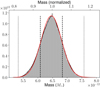 |
Fig. 1. Results of the MCMC algorithm applied to the synthetic [7,88;17186,46529,52443,7629,11701,142429] encounter for asteroid (7) Iris. Upperx-axis: normalized so that 1.0 equals the exact mass the data was generated with. The black dashed and dotted vertical lines represent the 1σ and 3σ limits, respectively, while the red graph corresponds to a Gaussian distribution based on the median and standard deviation of the results. |
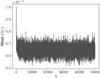 |
Fig. 2. Trace of the MCMC chain of the synthetic [7,88;17186,46529,52443,7629,11701,142429] encounter in terms of mass of asteroid (7) Iris. |
To further investigate the impact that additional perturbing and test asteroids have on the results, we investigated the mass of (7) Iris based on synthetic data with different combinations of asteroids. In the synthetic case, a single test asteroid is already sufficient to obtain very good mass estimates for (7) Iris, while the inclusion of additional test asteroids reduces the uncertainty of the results (Table 3). In addition, it is apparent that in this case the mass estimates for both (7) Iris and (88) Thisbe can be obtained based on their mutual perturbations alone, and no massless test asteroids are strictly necessary. The uncertainties resulting are, however, relatively wide, suggesting that their mutual perturbations are weak in comparison to those with their test asteroids. Finally, we see that it is not actually necessary to consider the perturbations of (88) Thisbe on (7) Iris to get good mass estimates of the latter. Nonetheless, including (88) Thisbe does further reduce the uncertainties of the mass of (7) Iris.
MCMC results for (7) Iris and (88) Thisbe based on synthetic data with different combinations of asteroids.
4.2. Real data
For our real data set, we did two separate MCMC runs for each case, one including the perturbations of Ceres, Pallas, and Vesta via the BC430 ephemerides (Baer & Chesley 2017) (Table 4), and one without (Table 5). These three asteroids were selected as they are by far the three most massive asteroids. In theory, the BC430 ephemeris permits us to include a significantly larger number of perturbers with pre-determined masses at the cost of increased computation time, but we expect that doing so will yield diminishing returns, due to the remaining asteroids having significantly lower masses. This is something we intend to investigate in greater detail in future work. For this study, we have checked the literature to ensure that our target asteroids have no published close encounters with other perturbers during the observation epoch. The run without BC430 perturbations was done to estimate the impact that asteroid perturbers can have on the results. The results including the BC430 perturbations should be considered our final results, because those results are based on a more accurate dynamical model. As with the previous synthetic test cases, a very small lower 3σ boundary can in practice be considered to be zero.
Compilation of the MCMC algorithm’s results including the perturbations of Ceres, Pallas, and Vesta for our real data set.
Our ML masses are typically close to the average literature values summarized by Carry (2012). In most test cases, these average values are well within our 1σ boundaries, whereas in Siltala & Granvik (2017), the literature values were typically only within the 3σ boundaries (Tables 4 and 5). One interesting exception to these results is (10) Hygiea, for which the significant differences between the results with and without BC430 are likely caused by at least one of the asteroids having close encounters with Ceres, Pallas or Vesta which, when not considered, lead to inaccurate orbits and masses.
Compilation of MCMC algorithm’s results without the perturbations of Ceres, Pallas, and Vesta for our real data set.
The mass estimates for asteroids (41) Daphne, (89) Julia, and (52) Europa have particularly wide uncertainties. The reason for this is that the perturbations on the test asteroid orbits from the close encounters used are quite weak. Zielenbach (2011) previously studied the first two of these targets using a much larger number of test asteroids and obtained significantly lower uncertainties in comparison to ours. We believe that including many more test asteroids would similarly reduce the formal uncertainties of our results for all three asteroids. However, the important aspect for this study is that the latest literature values are within the 1σ limits of our results, showing that the uncertainty estimates that we obtain are reliable.
Asteroid (16) Psyche is the target of NASA’s Psyche mission (Elkins-Tanton et al. 2014) and is commonly believed to be the iron core of a protoplanet. A recent bulk density estimate of approximately 4 g cm−3 given a mass estimate of (1.21 ± 0.16)×10−11 M⊙ (Viikinkoski et al. 2018) supports the theory that (16) Psyche is an iron core. However, our ML mass is significantly lower than the above estimate, and consequently points to a significantly lower bulk density than that reported in the literature (Fig. 3). This literature value nevertheless remains within our 3σ limits, and therefore our result does not rule out a significantly higher bulk density. Due to these interesting results, we chose to do a separate run for (16) Psyche in order to see whether this result can be reproduced with different test asteroids. Our ML masses from the two independent runs are similar, which shows that the small mass can indeed be reproduced with a different set of test asteroids (Table 4 and Fig. 3). We have also included a comparison between our results and previous studies (Viikinkoski et al. 2018) for Psyche (Fig. 4), which confirms that our nominal masses are indeed lower than all previous literature values, whereas our uncertainties are not unusually wide for this object.
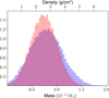 |
Fig. 3. Probability densities for the mass of (16) Psyche with BC430 perturbations for the cases of [16;17799,20837] (blue) and [16;91495,151878] (red). The upper x-axis shows the bulk density corresponding to the equivalent mass on the lower x-axis assuming a volume-equivalent diameter of 223 km (Table 4) corresponding to a volume of 5.806 × 10⁶ km3. We note that the volume uncertainty is not considered in this figure. |
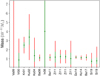 |
Fig. 4. Comparison of previous mass estimates for (16) Psyche based on asteroid-asteroid perturbations. References from left to right: Vasiliev & Yagudina (1999), Viateau (2000), Krasinsky et al. (2001), Kuzmanoski & Kovačević (2002), Kochetova (2004), Ivantsov (2008), Baer et al. (2008, 2011b), Zielenbach (2011), Goffin (2014), Kochetova & Chernetenko (2014), Baer & Chesley (2017); this work (Table 4). The green error bars represent 1σ limits, while the red error bars represent 3σ limits. |
The mean residuals for each asteroid in the [16;17799,20837] case show that there are no obvious systematic effects visible in the residuals that could explain the small ML mass (Figs. 5–7). We note that a few residuals are beyond the scale of the plots.
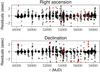 |
Fig. 5. Mean residuals of all accepted MCMC proposals for asteroid (16) Psyche in the case of [16;17799,20837]. The red crosses represent data that has been rejected as outliers and some outliers are entirely outside of the plot boundaries. |
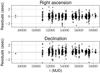 |
Fig. 6. Mean residuals of all accepted MCMC proposals for asteroid (17799) Petewilliams in the case of [16;17799,20837]. |
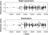 |
Fig. 7. Mean residuals of all accepted MCMC proposals for asteroid (20837) Ramanlal in the case of [16;17799,20837]. Red crosses represent data that has been rejected as outliers, and some outliers are entirely outside of the plot boundaries. |
To investigate the case of (16) Psyche further, we computed topocentric ephemerides for test asteroid (151878) 2003 PZ4 in the case of [16;91495,151878] several years into the future, and include the perturbations caused by (16) Psyche. This lets us quantify the impact of (16) Psyche’s perturbations on the test asteroid’s orbit, and to assess when astrometry should be obtained to efficiently constrain our mass estimate for (16) Psyche (Figs. 8 and 9). The behavior of RA around MJD 58650, corresponding to June 2019, where different perturber masses lead to ephemerides with differences up to two arcseconds resulting from the asteroid’s small distance from Earth, is particularly interesting. The uncertainty in the ephemeris prediction is driven by the uncertainty in perturber mass: a larger mass corresponds to a larger right ascension, while for declination there is little correlation (Figs. 10 and 11). In practice, this means that high-accuracy astrometry of asteroid (151878) 2003 PZ4 obtained during the summer of 2019 will significantly reduce the uncertainty of the mass estimate. The asteroid is easily observable during that time, and we thus expect that suitable astrometry will be obtained by asteroid surveys.
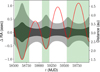 |
Fig. 8. Ephemeris prediction for asteroid (151878) 2003 PZ4 up to MJD 60000 in terms of RA relative to the best-fit value. The 1σ and 3σ credible intervals are shown in darker and lighter gray, respectively. The red line shows the asteroid’s topocentric distance as a function of time. The green color represents times when the asteroid is observable assuming a topocentric observer, by requiring that the solar elongation is greater than 60 degrees, and the apparent V magnitude is less than 21. |
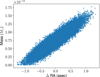 |
Fig. 10. Mass of (16) Psyche versus the RA prediction for asteroid (151878) 2003 PZ4 relative to best-fit value at MJD 58650. |
Although our ML masses have improved, partly due to additional data, our uncertainties tend to be wider than in Siltala & Granvik (2017) (Table 4). We believe this is largely caused by the different observational weights used; in particular, the  term, which was not used in our previous work, directly leads to much looser weights for some observations, which translates to greater uncertainties in the results. To demonstrate this effect, we also chose to test MCMC without the
  factor applied in the error model (Table 6). Upon comparison with results including the factor (Table 4), it is clear that the factor does indeed increase the uncertainties of our test cases as expected.
Results of the MCMC algorithm for data without the  factor.
To assess the impact of multiple simultaneous test asteroids on our results, we also chose to run our algorithm for each test asteroid separately for some of these cases (Tables 7 and 8). In general, these results also show clear improvement in comparison to our previous study, as the ML masses now tend to be significantly closer to the average literature value. We do, however, note the case of [10;1259], where our ML mass is clearly unrealistic in Table 8, being an order of magnitude above even the mass of Ceres. Furthermore, [29;7060] and [52;306] exhibit similar behavior, but these two cases also have extremely wide uncertainties, and the previous literature values easily fall within these. We suspect that in the latter two cases, the perturbations are simply very weak, directly resulting in very high noise, making these particular encounters quite poor for mass estimation. Indeed, comparing these values to those in Table 5, we see that the “better” encounters dominate in the cases with both test asteroids combined, which is to be expected.
Compilation of the MCMC algorithm’s results including perturbations of Ceres, Pallas and Vesta for several cases from our real data set separately for each test asteroid.
Compilation of the MCMC algorithm’s results without the perturbations of Ceres, Pallas, and Vesta for several cases from our real data set separately for each test asteroid.
The inclusion of perturbations of Ceres, Pallas and Vesta has a significant impact on [10;1259] (Table 7); where previously the ML mass was an order of magnitude above that of Ceres, it is now much closer to the literature values, though the noise level remains high. This appears to confirm that (1259) Ogyalla has a close encounter with at least one of these three perturbers during the observational timespan, though we are not aware of any previously published information on such an encounter. The cases of [29;7060] and [52;306], however, remain extremely noisy.
To show how two simultaneous test asteroids improve the mass estimate compared to two separate runs with a single test asteroid each, for the example case of (16) Psyche, we have included a figure showcasing our results with two simultaneous test asteroids compared with results for each test asteroid considered separately (Fig. 12). The peak of the distribution for both test asteroids combined, corresponds to the peak of the overlapping part of the separate single-test-asteroid distributions, which was our expectation. This essentially means that the maximum likelihood value for the mass in the former case corresponds to the mass that best fits both separate test asteroids simultaneously.
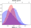 |
Fig. 12. Probability densities for the mass of (16) Psyche with BC430 perturbations for two simultaneous test asteroids (17799 and 20837, red), and two cases with each test asteroid considered separately (blue). Upper x-axis: bulk density corresponding to the equivalent mass on the lower x-axis, assuming a volume-equivalent diameter of 223 km (Drummond et al. 2018). |
In order to study how increasing the number of data points affects the resulting mass distributions, we opted to perform MCMC runs with approximately half the observational timespan to limit the number of astrometry used for the cases of [15;765] and [15;765,14401] (Table 9) where, for reference, the encounter with the former test asteroid took place in 2010, and the latter in 2005 (Galád & Gray 2002). Here, one can see that for the case of [15;765,14401], cutting the observational timespan to half slightly increases the uncertainty of the mass, while for [15;765] alone the change is slightly greater. Using a timespan of 2003-2007, the result for [15;765] becomes essentially useless, which is expected given that no close encounters between these two asteroids exist in this time period. While we did not perform the computation for [15;14401] in this case, it is clear that this test asteroid dominates the results of [15;765,14401] and would be expected to provide essentially the same result. Overall, these results do indeed show that additional data significantly reduces the uncertainties of the mass, as is expected.
Comparison of MCMC results of [15;765,14401] and [15;765] with differing observational timespans.
5. Conclusions
We have successfully developed, implemented, and validated a robust adaptive Metropolis algorithm for asteroid mass estimation. Our results show significant improvement compared to our previous work (Siltala & Granvik 2017) with the new RAM algorithm, the ability to include multiple perturbers and test asteroids simultaneously, the improved force model, and the new observational weighting scheme. The uncertainties remain wider than recent previous literature values, while in almost all cases, the literature values are within our 1σ limits.
The interesting exception is (16) Psyche, for which we obtain a significantly smaller mass than previously reported in the literature. Given that we find consistent results with two independent data sets–less the data set for (16) Psyche itself–this result merits further analysis when additional data on (151878) 2003 PZ4 is obtained later this year.
In the future, we intend to extend OpenOrb so that we can use Gaia astrometry in combination with ground-based astrometry for asteroid mass estimation.
Acknowledgments
This work was supported by grants #299543, #307157, and #328654 from the Academy of Finland. This research has made use of NASA’s Astrophysics Data System, and data and/or services provided by the International Astronomical Union’s Minor Planet Center. We thank the anonymous referee for their useful comments which greatly improved our paper. We would also like to thank James Baer and William Zielenbach for their answers to our questions about their respective works and the latter also for providing us with lists of close encounters with three of our target perturbers. The computations for this work were mainly performed with the Kale cluster of the Finnish Grid and Cloud infrastructure (persistent identifier: urn:nbn:fi:research-infras-2016072533), and the scientific computing environment of the Nordic Optical Telescope set up by Peter Sorensen.
References
- Andrieu, C., & Thoms, J. 2008, Stat. Comput., 18, 343 [CrossRef] [Google Scholar]
- Baer, J., & Chesley, S. R. 2017, AJ, 154, 76 [NASA ADS] [CrossRef] [Google Scholar]
- Baer, J., Milani, A., Chesley, S., & Matson, R. D. 2008, in An Observational Error Model, and Application to Asteroid Mass Determination, AAS/Division Planet. Sci. Meet. Abstracts, 40, 52.09 [Google Scholar]
- Baer, J., Chesley, S. R., & Milani, A. 2011a, Icarus, 212, 438 [NASA ADS] [CrossRef] [Google Scholar]
- Baer, J., Chesley, S. R., & Matson, R. D. 2011b, AJ, 141, 143 [NASA ADS] [CrossRef] [Google Scholar]
- Carry, B. 2012, Planet. Space Sci, 73, 98 [NASA ADS] [CrossRef] [Google Scholar]
- Chesley, S. R., Chodas, P. W., Milani, A., Valsecchi, G. B., & Yeomans, D. K. 2002, Icarus, 159, 423 [NASA ADS] [CrossRef] [Google Scholar]
- Drummond, J. D., Merline, W. J., Carry, B., et al. 2018, Icarus, 305, 174 [NASA ADS] [CrossRef] [Google Scholar]
- Elkins-Tanton, L. T., Asphaug, E., Bell, J., et al. 2014, in Journey to a Metal World: Concept for a Discovery Mission to Psyche, Lunar Planet. Sci. Conf., 45, 1253 [Google Scholar]
- Farnocchia, D., Chesley, S. R., Chamberlin, A. B., & Tholen, D. J. 2015a, Icarus, 245, 94 [NASA ADS] [CrossRef] [Google Scholar]
- Farnocchia, D., Chesley, S., & Micheli, M. 2015b, Icarus, 258, 18 [NASA ADS] [CrossRef] [Google Scholar]
- Gaia Collaboration (Brown, A. G. A., et al.) 2018a, A&A, 616, A1 [NASA ADS] [CrossRef] [EDP Sciences] [Google Scholar]
- Gaia Collaboration (Spoto, F., et al.) 2018b, A&A, 616, A13 [NASA ADS] [CrossRef] [EDP Sciences] [Google Scholar]
- Galád, A., & Gray, B. 2002, A&A, 391, 1115 [NASA ADS] [CrossRef] [EDP Sciences] [Google Scholar]
- Goffin, E. 2014, A&A, 565, A56 [NASA ADS] [CrossRef] [EDP Sciences] [Google Scholar]
- Granvik, M., Virtanen, J., Oszkiewicz, D., & Muinonen, K. 2009, Meteorit. Planet. Sci., 44, 1853 [NASA ADS] [CrossRef] [Google Scholar]
- Haario, H., Saksman, E., & Tamminen, J. 2001, Bernoulli, 7, 223 [CrossRef] [MathSciNet] [Google Scholar]
- Hanuš, J., Viikinkoski, M., Marchis, F., et al. 2017, A&A, 601, A114 [NASA ADS] [CrossRef] [EDP Sciences] [Google Scholar]
- Ivantsov, A. 2008, Planet. Space Sci., 56, 1857 [NASA ADS] [CrossRef] [Google Scholar]
- Kochetova, O. M. 2004, Sol. Syst. Res., 38, 66 [NASA ADS] [CrossRef] [Google Scholar]
- Kochetova, O. M., & Chernetenko, Y. A. 2014, Sol. Syst. Res., 48, 295 [NASA ADS] [CrossRef] [Google Scholar]
- Krasinsky, G. A., Pitjeva, E. V., Vasiliev, M. V., & Yagudina, E. I. 2001, in Estimating masses of asteroids, Communications of IAA of RAS [Google Scholar]
- Kuzmanoski, M., & Kovačević, A. 2002, A&A, 395, L17 [NASA ADS] [CrossRef] [EDP Sciences] [Google Scholar]
- Roberts, G. O., Gelman, A., & Gilks, W. R. 1997, Ann. Appl. Probab., 7, 110 [CrossRef] [Google Scholar]
- Siltala, L., & Granvik, M. 2017, Icarus, 297, 149 [NASA ADS] [CrossRef] [Google Scholar]
- Vasiliev, M., & Yagudina, E. 1999, Determination of masses for 26 selected minor planets from analysis of observations their mutual encounters with asteroids of lesser mass. Communications of IAA of RAS [Google Scholar]
- Vernazza, P., Brož, M., Drouard, A., et al. 2018, A&A, 618, A154 [NASA ADS] [CrossRef] [EDP Sciences] [Google Scholar]
- Viateau, B. 2000, A&A, 354, 725 [NASA ADS] [Google Scholar]
- Vihola, M. 2012, Stat. Comput., 22, 997 [CrossRef] [Google Scholar]
- Viikinkoski, M., Hanuš, J., Kaasalainen, M., Marchis, F., & Ďurech, J. 2017, A&A, 607, A117 [NASA ADS] [CrossRef] [EDP Sciences] [Google Scholar]
- Viikinkoski, M., Vernazza, P., Hanuš, J., et al. 2018, A&A, 619, L3 [NASA ADS] [CrossRef] [EDP Sciences] [Google Scholar]
- Zielenbach, W. 2011, AJ, 142, 120 [NASA ADS] [CrossRef] [Google Scholar]
All Tables
MCMC results for (7) Iris and (88) Thisbe based on synthetic data with different combinations of asteroids.
Compilation of the MCMC algorithm’s results including the perturbations of Ceres, Pallas, and Vesta for our real data set.
Compilation of MCMC algorithm’s results without the perturbations of Ceres, Pallas, and Vesta for our real data set.
Compilation of the MCMC algorithm’s results including perturbations of Ceres, Pallas and Vesta for several cases from our real data set separately for each test asteroid.
Compilation of the MCMC algorithm’s results without the perturbations of Ceres, Pallas, and Vesta for several cases from our real data set separately for each test asteroid.
Comparison of MCMC results of [15;765,14401] and [15;765] with differing observational timespans.
All Figures
|
Fig. 1. Results of the MCMC algorithm applied to the synthetic [7,88;17186,46529,52443,7629,11701,142429] encounter for asteroid (7) Iris. Upperx-axis: normalized so that 1.0 equals the exact mass the data was generated with. The black dashed and dotted vertical lines represent the 1σ and 3σ limits, respectively, while the red graph corresponds to a Gaussian distribution based on the median and standard deviation of the results. |
| In the text | |
|
Fig. 2. Trace of the MCMC chain of the synthetic [7,88;17186,46529,52443,7629,11701,142429] encounter in terms of mass of asteroid (7) Iris. |
| In the text | |
|
Fig. 3. Probability densities for the mass of (16) Psyche with BC430 perturbations for the cases of [16;17799,20837] (blue) and [16;91495,151878] (red). The upper x-axis shows the bulk density corresponding to the equivalent mass on the lower x-axis assuming a volume-equivalent diameter of 223 km (Table 4) corresponding to a volume of 5.806 × 10⁶ km3. We note that the volume uncertainty is not considered in this figure. |
| In the text | |
|
Fig. 4. Comparison of previous mass estimates for (16) Psyche based on asteroid-asteroid perturbations. References from left to right: Vasiliev & Yagudina (1999), Viateau (2000), Krasinsky et al. (2001), Kuzmanoski & Kovačević (2002), Kochetova (2004), Ivantsov (2008), Baer et al. (2008, 2011b), Zielenbach (2011), Goffin (2014), Kochetova & Chernetenko (2014), Baer & Chesley (2017); this work (Table 4). The green error bars represent 1σ limits, while the red error bars represent 3σ limits. |
| In the text | |
|
Fig. 5. Mean residuals of all accepted MCMC proposals for asteroid (16) Psyche in the case of [16;17799,20837]. The red crosses represent data that has been rejected as outliers and some outliers are entirely outside of the plot boundaries. |
| In the text | |
|
Fig. 6. Mean residuals of all accepted MCMC proposals for asteroid (17799) Petewilliams in the case of [16;17799,20837]. |
| In the text | |
|
Fig. 7. Mean residuals of all accepted MCMC proposals for asteroid (20837) Ramanlal in the case of [16;17799,20837]. Red crosses represent data that has been rejected as outliers, and some outliers are entirely outside of the plot boundaries. |
| In the text | |
|
Fig. 8. Ephemeris prediction for asteroid (151878) 2003 PZ4 up to MJD 60000 in terms of RA relative to the best-fit value. The 1σ and 3σ credible intervals are shown in darker and lighter gray, respectively. The red line shows the asteroid’s topocentric distance as a function of time. The green color represents times when the asteroid is observable assuming a topocentric observer, by requiring that the solar elongation is greater than 60 degrees, and the apparent V magnitude is less than 21. |
| In the text | |
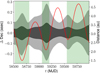 |
Fig. 9. As Fig. 8, but for Dec. |
| In the text | |
|
Fig. 10. Mass of (16) Psyche versus the RA prediction for asteroid (151878) 2003 PZ4 relative to best-fit value at MJD 58650. |
| In the text | |
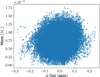 |
Fig. 11. As Fig. 10, but for Dec instead of RA. |
| In the text | |
|
Fig. 12. Probability densities for the mass of (16) Psyche with BC430 perturbations for two simultaneous test asteroids (17799 and 20837, red), and two cases with each test asteroid considered separately (blue). Upper x-axis: bulk density corresponding to the equivalent mass on the lower x-axis, assuming a volume-equivalent diameter of 223 km (Drummond et al. 2018). |
| In the text | |
Current usage metrics show cumulative count of Article Views (full-text article views including HTML views, PDF and ePub downloads, according to the available data) and Abstracts Views on Vision4Press platform.
Data correspond to usage on the plateform after 2015. The current usage metrics is available 48-96 hours after online publication and is updated daily on week days.
Initial download of the metrics may take a while.