| Issue |
A&A
Volume 633, January 2020
|
|
|---|---|---|
| Article Number | A91 | |
| Number of page(s) | 10 | |
| Section | Extragalactic astronomy | |
| DOI | https://doi.org/10.1051/0004-6361/201935602 | |
| Published online | 16 January 2020 | |
Modelling the Canes Venatici I dwarf spheroidal galaxy
1
Departamento de Astronomía, Universidad de Concepción, Casilla 160-C, 3340 Concepción, Chile
e-mail: This email address is being protected from spambots. You need JavaScript enabled to view it.
2
Observatories of the Carnegie Institution of Washington, 813 Santa Barbara St., Pasadena, CA 91101, USA
Received:
2
April
2019
Accepted:
18
November
2019
Abstract
The aim of this work is to find a progenitor for Canes Venatici I (CVn I), under the assumption that it is a dark matter free object that is undergoing tidal disruption. With a simple point mass integrator, we searched for an orbit for this galaxy using its current position, position angle, and radial velocity in the sky as constraints. The orbit that gives the best results has the pair of proper motions μα = −0.099 mas yr−1 and μδ = −0.147 mas yr−1, that is, an apogalactic distance of 242.79 kpc and a perigalactic distance of 20.01 kpc. Using a dark matter free progenitor that undergoes tidal disruption, the best-fitting model matches the final mass, surface brightness, effective radius, and velocity dispersion of CVn I simultaneously. This model has an initial Plummer mass of 2.47 × 10⁷ M⊙ and a Plummer radius of 653 pc, producing a remnant after 10 Gyr with a final mass of 2.45 × 10⁵ M⊙, a central surface brightness of 26.9 mag arcsec−2, an effective radius of 545.7 pc, and a velocity dispersion with the value 7.58 km s−1. Furthermore, it is matching the position angle and ellipticity of the projected object in the sky.
Key words: methods: numerical / galaxies: dwarf / galaxies: individual: CVn I
© ESO 2020
1. Introduction
Dwarf spheroidal (dSph) galaxies are one of the most abundant objects in the Universe (Mateo 1998; Metz & Kroupa 2007). As the name implies, dSph are small galaxies, with a low stellar content. They have low amounts of gas or even lack it completely, have no star formation, and have a population of very old (>10 Gyr) and metal poor (−3 < [Fe/H] < 0) stars (Mateo 1998; McConnachie 2012). According to the Λ Cold Dark Matter model, massive galaxies, like the Milky Way (MW), should be surrounded by large numbers of dark matter (DM) dominated satellites (Simon & Geha 2007). Their small number of stars makes them very faint, with absolute magnitudes between −13 ≤ MV ≤ −7 magnitudes (Mateo 1998; Belokurov et al. 2007), and hard to detect (Tollerud et al. 2008); ∼50 of them are identified as satellites of the MW (McConnachie 2012; Koposov et al. 2015; Newton et al. 2018). Despite their low luminous mass, dSphs have high velocity dispersions (Mateo 1998; Simon & Geha 2007). Assuming virial equilibrium, spherical symmetry, and isotropic velocity dispersion, the dynamical mass of these galaxies is of the order of 107–108 M⊙, within their half-light radius. Since the dynamical mass is much higher than the luminous mass (stars), the general consensus is that they contain a high amount of DM. In fact they are the objects with the highest concentration of DM in the Universe, reaching mass-to-light ratios (M/Ls) of ∼100 or even ∼1000 (Simon & Geha 2007).
Located near the North Galactic Pole at a distance of 224 kpc from the Earth (Zucker et al. 2006), the Canes Venatici I dwarf spheroidal galaxy (CVn I dSph, α0 = 13h28m03.5s, δ0 = 33°33′21.0″) was, at the moment of its discovery, one of the most remote satellites to the MW (Zucker et al. 2006). Being a relatively luminous companion to the MW (Mv = −7.9 ± 0.5 mag; Zucker et al. 2006), its large distance allowed it to remain undetected until 2006. With a half-light radius of 564 pc (Zucker et al. 2006), it is one of the largest satellites of the MW (McConnachie 2012; Zucker et al. 2006). It possesses an old (∼12 Gyr, Okamoto et al. 2012), metal-poor ([Fe/H] ∼ −2 (Zucker et al. 2006; Simon & Geha 2007) population of stars that represents 95% of the luminous mass of the galaxy, and a younger (∼1.4−2.0 Gyr) more metal-rich ([Fe/H] ∼ −1.5,) population of stars, revealed by a blue plume in the galaxy’s colour-magnitude diagramme (Martin et al. 2008a), accounting for the remaining 5% of the stars.
As commonly observed in this type of galaxies (Mateo 1998), CVn I has a high velocity dispersion, with a value of 7.6 km s−1 (Simon & Geha 2007). If one assumes virial equilibrium, spherical symmetry, and isotropic velocity dispersion, this value indicates a virial mass of 2.7 × 10⁷ M⊙ and, therefore, a M/L ∼ 220 (Simon & Geha 2007), suggesting that the internal dynamics of this galaxy are dominated by a DM halo. The line-of-sight velocity of CVn I is given in Simon & Geha (2007) and amounts to 30.9 ± 0.6 km s−1. In a recent publication Fritz et al. (2018) used the Gaia DR2 data to determine a possible proper motion of the dwarf. They calculate μα = −0.159 ± 0.094 ± 0.035 mas yr−1 and μδ = −0.067 ± 0.054 ± 0.035 mas yr−1.
As noted on different occasions (Zucker et al. 2006; Okamoto et al. 2012; Martin et al. 2008b), the CVn I dSph has an elongated shape, with a ellipticity of ϵ = 0.38. In Fig. 8 of Okamoto et al. (2012), we see that it is a very flattened and elongated system. Part of this elongation may be due to the onset of tidal tails, that is the object would be heavily influenced by Galactic tides.
It has been shown that tidally disrupted objects have their line-of-sight velocity dispersions boosted by unbound stars that form the tidal tails (Read et al. 2006; Muñoz et al. 2008; Klimentowski et al. 2009; Smith et al. 2013a; Blaña et al. 2015). This boost is strongest if the object is observed near its apo-centre, where objects spend most of their orbital time according to Kepler’s second law. This increased value, under the assumption of virial equilibrium, leads to an overestimation of the dynamical mass of the system and to an elevated M/L.
According to some astronomers, the presence of a disc of satellites around the MW (Pawlowski et al. 2012) and M31 (Ibata et al. 2013) suggests that each of these galaxies may have suffered a major interaction at some point in their past (Sawa & Fujimoto 2005; Pawlowski et al. 2011; Fouquet et al. 2012; Hammer et al. 2013). One possibility is that CVn I might have been formed as a small tidal dwarf galaxy (TDG; Duc 2012) in such an interaction. Simulations show that these second generation objects can form from tidal interactions between galaxies (Wetzstein et al. 2007; Bournaud et al. 2008; Ploeckinger et al. 2018) and survive the initial stages of their formation (Recchi et al. 2007; Ploeckinger et al. 2014) up to several Gyr (Bournaud et al. 2003). Also, observations indeed show that not only are these kinds of objects formed in galaxy interactions (Kaviraj et al. 2012; Scott et al. 2018), but they can survive several Gyr around their progenitors (Duc et al. 2014). If that is the case, then Canes Venatici I might not be a DM-dominated object, since the gravitational collapse of the material that forms a tidal tail produces an object that is unable to capture any DM particle (Bournaud 2010).
A DM dominated dSph must lose ∼90% of its dark matter halo before the luminous part can be affected by the gravitational influence of the MW (Smith et al. 2013b). If Canes Venatici I is affected and elongated by tides, then even though it would have been DM dominated in the past, DM is not the cause for the high velocity dispersion we see today.
Dwarf disc interactions (Mayer et al. 2007; D’Onghia et al. 2009) work for larger dwarfs, that is reducing the stellar content and reshaping it while at the same time leaving the DM halo more or less intact, but faint and ultra faint dSph may not have formed from dwarf discs as they have very low mass haloes with circular velocities in the order of or below the velocity dispersion expected (Hazeldine & Fellhauer 2018, priv. comm.).
The aim of this project is to find a possible DM free progenitor, able to reproduce the observed properties of CVn I mentioned above and shown in Table 1. In the next section, we explain the setup of our simulations followed by our results. We end this paper with some conclusions and briefly discussing our results.
Observable properties of CVn I.
2. Setup
2.1. Infall time
The “infall time” denotes the starting point of the simulations. As dSph have an old and metal-poor population of stars, meaning that they stopped creating new ones long time ago, this starting point should reflect the time when the majority of the stars were created. Spectroscopic data shows that CVn I dSph is dominated by an old and metal-poor stellar population (Zucker et al. 2006), and isochrone fitting indicates that the age of these stars is at least 10 Gyr old, with a younger population of ∼1.2–2.0 Gyr that makes up to ∼5% of the mass of the galaxy (Martin et al. 2008a). We use this value as a reference to chose a generic “infall time” of 10 Gyr, to account for the fact that we do not know the true value for this parameter.
We use the term “infall time” for the start of our simulations, even though it might be misleading. If CVn I was indeed originally a DM dominated dwarf galaxy, the start of our simulations marks the point in its evolution, where most of the DM halo (>90%) was already stripped away in the past. In the case that CVn I was DM free from its formation, we might be looking at a tidal dwarf galaxy which has formed orbiting the MW instead of falling in.
Previous studies (e.g. Blaña et al. 2015) show that a change in “infall time” (e.g. from 10 to 5 Gyr) does not alter our conclusions, that is it is possible to reproduce the observables of a dSph with a DM-free object. It just changes the properties of the progenitor, which can be less massive or less concentrated to begin with, as it needs less time to survive the tidal forces of the MW.
2.2. Orbit candidates
The trajectory of a particle in the potential of the MW is completely defined if one knows the 3D position and the 3D velocity vectors. Using a point mass integrator (PMI) it is possible to integrate backwards in time to obtain the path of the galaxy and its position and velocity 10 Gyr ago, with the resulting values as initial conditions at the beginning of the simulation, using potentials to model the MW following Mizutani et al. (2003).
The galactic disc was modelled using the Miyamoto-Nagai (Miyamoto & Nagai 1975) profile, defined as:
![Mathematical equation: $$ \begin{aligned} \Phi ^\mathrm{MN}_{\rm disc}(R,z) = \frac{-GM_{\mathrm{disc} }}{\left( R^2+\left[a+(z^2+b^2)^{1/2}\right]^2\right)^{1/2}} \end{aligned} $$](/articles/aa/full_html/2020/01/aa35602-19/aa35602-19-eq1.gif) (1)
(1)
where the parameters are Mdisc = 1011 M⊙, a = 6.5 kpc and b = 0.26 kpc. To describe the bulge of the MW, the Hernquist model (Hernquist 1990) was used:
 (2)
(2)
with c = 0.7 kpc and Mbulge = 3.4 × 10¹⁰ M⊙. At the distance where CVn I dSph is currently located, the DM halo of the MW is nearly spherical (Fellhauer et al. 2006), so a logarithmic halo was chosen to model this structure:
 (3)
(3)
where the values of the parameters are v0 = 131.5 km s−1 and d = 12 kpc.
For CVn I dSph we know its position in the sky, its distance to the Sun and its velocity in the line-of-sight, that is the three components of its position vector and only one component of the velocity vector. The two proper motions of the galaxy as seen from Earth are still needed to compute a possible orbit: along the declination axis (μδ) and along the right ascension axis (μα).
Even though there is an infinite number of pairs (μα, μδ), using the fact that galaxies that are not DM dominated (either because they lost their DM or were born without it) and are undergoing tidal disruption will show tidal tails along their orbit, leaves us with only those pairs of proper motion, generating orbits parallel to the projected major axis of the elongated dSph. In Fig. 1 we show the past position of the test particle as the red line and the future position as the green line.
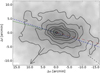 |
Fig. 1. Projected orbit of CVn I dSph on the sky. The red dashed line represents the past position of CVn I dSph, while the green line corresponds to the future position of the galaxy. The blue dots are aligned to the major axis of the dwarf. The isodensity contour plot was adapted from Okamoto et al. (2012), Fig. 8. |
That tidal tails are aligned with the orbit is true if we see the object close to its apo-centric distance. On an eccentric orbit, objects lose stars while going through peri-centre or due to tidal shocks passing the disc of the main galaxy. The particles (stars) leave the object through the Lagrangian points L1 and L2, that is perpendicular to their orbits. These newly lost particles will align with the orbit on the way out to the apo-centre.
Old tails stay aligned with the orbit, which may lead to strange appearances, closely after peri-centre, of 4 tails, a phenomenon which Blaña et al. (2015) dubbed “X-wing” shape. A similar behaviour is quoted in Klimentowski et al. (2009), even though they are using a dwarf disc galaxy embedded in a dark matter halo. They see that the new tidal tails emerge perpendicular to the orbit after the peri-centre passage and align with the orbit during the later evolution. In contrast to objects like star clusters or in general spherical, dispersion supported objects without dark matter, like in this study, they discuss that in their case the alignment needs longer time and their tails are still perpendicular at apo-centric distances.
The velocity dispersion of the galaxy is boosted when it reaches apogalacticon (Smith et al. 2013a), so a second condition that the final orbit must satisfy is that the apogalactic distance must be close to the current distance of CVn I dSph.
The possible pairs of proper motions are selected from the intersection of the regions, found using the method described in Appendix A, that satisfy the criteria mentioned above. These candidates are summarised in Table 2 and shown in Fig. 2. The blue dotted line represents the pairs of proper motions that match the position angle of CVn I, while the purple, red, green, and yellow dotted circles mark the zone of parameter space where the orbits have apogalactic distances of 245 kpc, 244 kpc, 243 kpc, and 242.5 kpc, respectively. The black crosses are the candidates for the final orbit (Table 2), while the red plus sign is the selected orbit. Orbits in the centre of the concentric circles have the smallest apogalactic and perigalactic distance, with 242.2 kpc and 7.8 kpc, respectively, but they do not match the position angle of the galaxy.
Candidates for the CVn I dSph orbit.
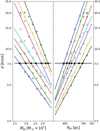 |
Fig. 2. Proper motions of the orbit candidates. The blue dots represent the pairs of proper motions that match the position angle of CVn I, while the purple, red, green, and yellow dotted circles mark the zone of parameter space where the orbits have apogalactic distances of 245 kpc, 244 kpc, 243 kpc, and 242.5 kpc, respectively. The black crosses are the candidates for the final orbit (Table 2), while the red plus sign is the selected orbit. |
For each of the candidates of Table 2 we run one simulation for 10 Gyr, using a Plummer sphere with a scale length (Plummer radius Rpl) of 630 pc and a total mass of Mpl = 2.13 × 10⁷ M⊙, distributed into one million particles. We use Superbox (Fellhauer et al. 2000), a particle-mesh code, where a sub-grid with a spatial resolution of Rcore = RPl/15 was selected to ensure that these models are stable in isolation. In a particle-mesh code it is possible to use an arbitrary number of particles as they represent phase-space elements and not single stars.
From the output of the test models, we choose the orbit whose simulation ended with a remnant with values closest to the ones observed in CVn I dSph, so the orbit (2) from Table 2 is the one that we use. This orbit has a perigalactic distance of 20.013 kpc and apogalactic distance of 242.79 kpc, which gives us an eccentricity of ϵ ∼ 0.85 and three pericentric passages within the 10 Gyr of simulation. With our choice of proper motions of μα = −0.099 mas yr−1 and μδ = −0.147 mas yr−1 we are within the 1σ-errors of the recently determined proper motions by Fritz et al. (2018) using the Gaia DR2 data. This is by coincidence as at the start of our study, these values were not yet available. The initial position and velocity of the progenitor, according to the chosen orbit, are shown in Table 3 and Fig. 3.
Parameters of the chosen orbit.
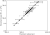 |
Fig. 3. Selected orbit for CVn I. The green line shows the position of the point mass particle backwards in time, the blue square the position at t = −10 Gyr and the red triangle the current position of CVn I. Axes centred on the Galactic centre. |
2.3. Initial conditions
We model our DM-free progenitor of CVn I, using the chosen orbit, again as a Plummer sphere (Plummer 1911) with similar properties as the test model used to select the orbit: made of one million, equal mass particles and using a sub-grid with spatial resolution of Rpl/15. In contrast to the previous subsection we now use the same orbit but we vary the parameters of the Plummer sphere, that is the Plummer radius Rpl and the total mass of the object Mpl, to find the best matching final object. A total of 147 Plummer spheres were used, divided into 3 sets with 7 radii and 7 masses each, so that each set has 49 models. A summary of the properties of the used Plummer spheres can be found in Table 4.
Plummer radius and Plummer masses of each set of simulations.
To reach the goal of finding the initial Plummer radius Rpl and initial mass Mpl of a Plummer sphere that, after 10 Gyr orbiting the MW on the path chosen above, will generate a remnant that reproduces the current observable parameters of CVn I dSph, it is necessary to understand how these observables are affected by Rpl and Mpl. This will be explained in more detail in the following section.
3. Results and final object
The remnants are analysed to find any trends that will help to constrain the initial conditions of CVn I dSph. We follow the method detailed in Domínguez et al. (2016) and Blaña et al. (2015). In this method instead of trial and error to get better and better matches of all observables simultaneously, we search for functions of initial parameter sets which fit a certain observable independently of the others. The observational parameters of the dwarf that we are trying to match can be found in Table 1.
When we are trying to fit a single observational parameter, we only take its observational value into account and not the observational errors that are given in Table 1. As will be shown in the following subsections, our mathematical errors due to fitting procedures in logarithmic space are much larger that the tight relations they accompany. We believe that the extra observational errors would only enlarge the error-bars by a small factor.
3.1. Mass
The mass estimates for CVn I dSph available in the literature were calculated under the assumption that this object is spherical, is in dynamical equilibrium, and has an isotropic velocity dispersion. From this, one gets a mass in the order of 2.7 × 10⁷ M⊙ and a M/L of 221 (Simon & Geha 2007), and, therefore, a DM-dominated object. Since we are trying to model this galaxy as a DM-free object, we cannot use that value as the mass that needs to be matched. Instead, a generic mass-to-light ratio equal to one is used to transform the observed luminosity of CVn I dSph to an estimate of its luminous mass.
Martin et al. (2008b) reports that the total luminosity of CVn I dSph is 2.3 × 10⁵ L⊙. Using the M/L mentioned above, the luminous mass of this galaxy (and the mass that our models have to reach) would be 2.3 × 10⁵ M⊙. The mass calculated above uses all the light that comes from the galaxy, that is not only the stars that are still gravitationally bound, but also any tidal debris that might be in the vicinity. Following this principle, to measure the mass of the object at the end of the simulation, we add the masses of all the particles inside a box that covers ±20′ in Dec and ±20′ in RA around the centre of density of the remnant, similar to the area observed by Martin et al. (2008a).
In Fig. 4 we plot the measured final masses of our objects as function of their initial Mpl (left panel) and Rpl (right panel) respectively. In the left panel, all points with the same symbol have the same value for Rpl, showing how the final mass depends on the initial mass for each choice of Rpl. As expected, a body with higher initial mass will produce a more massive remnant, as the additional material will help to resist the tidal influence of the MW. In the right panel, all points with the same symbol have the same value for Mpl, showing how the final mass depends on the Plummer radius. Models with larger radii lose more mass than the more compact ones since these are more loosely bounded and more easily disrupted.
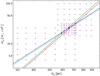 |
Fig. 4. Final mass as a function of the initial parameters of the model. Left: final mass as a function of the initial mass. Shown here are the data points and fitting lines for Plummer radii of 560 (blue dots), 610 (green triangles), 660 (red squares), 710 (cyan diamonds), 760 (magenta stars), 830 (yellow circles), and 890 pc (black triangles). Right: final mass as a function of the Plummer radius. Shown here are the data point and fitting lines for Plummer masses of 17.37 × 10⁶ (blue circles), 19.2 × 10⁶ (green triangles), 21.21 × 10⁶ (red squares), 23.44 × 10⁶ (cyan diamonds), 25.9 × 10⁶ (magenta stars), 28.61 × 10⁶ (yellow circles), and 31.62 × 10⁶ M⊙ (black triangles). Horizontal solid line denotes the adopted value of the final mass that needs to be matched. The black squares are the matching values calculated by fitting power laws to the data points. |
For models with the same radius Rpl, the points form a straight line in this double logarithmic plot. We fitted a power law of the form log10Mfin = A ⋅ log10Mpl + B and find the value of Mpl for which Mfin = 2.3 × 10⁵ M⊙. From this we obtain the pair (Rpl, Mpl) that will generate a model that, at the end of the simulation, will have a final mass with the desired value.
This is done for all sets with equal Plummer radius and then for all the sets with equal Plummer mass (Fig. 4, right panel). These (Rpl, Mpl) pairs are, then, plotted in a graph of Plummer mass vs Plummer radius with logarithmic axes (Fig. 5), where the points also form a straight line that can be fitted with a power law. These points have error bars in only one direction, as the value in one of the directions is given by the initial conditions of the simulation, while the other stems from fitting a power law to a set of points. Any points in this power law will produce a remnant with a final mass close to 2.3 × 10⁵. The power law for this observable is:
![Mathematical equation: $$ \begin{aligned} M_{\rm pl}[{M}_\odot ] = 0.83 \pm 0.7 \times R^{2.65 \pm 0.01}_{\rm pl}\, [\mathrm{pc} ]. \end{aligned} $$](/articles/aa/full_html/2020/01/aa35602-19/aa35602-19-eq4.gif) (4)
(4)
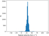 |
Fig. 5. Pairs of initial parameters which lead to final models with the correct mass of Canes Venatici I dSph. |
The large error bars in this figure are due to the fitting procedure to obtain the corresponding initial values. A fitting line from Fig. 4 has an error in the zero-point and another in the slope. Both errors can affect the fitted value of the searched for second initial parameter. Even though we seemingly have done a better job with our simulations, as the almost perfectly aligned data points suggest, we give the correct mathematical uncertainties.
Once again we stress that in the fitting routine we only consider the observational value given in Table 1 and pay no consideration to the associated observational error. Doing so would only enlarge our already large mathematical errors. The same reasoning will be used in fitting the other observables as well.
3.2. Surface brightness
The same region used to measure the final mass of the object (see Sect. 3.1) was used now to create a map of the surface mass density with a resolution of 0.02° px−1. The same generic M/L = 1 was used to convert the surface densities (measured in [M⊙pc−2]) into surface brightness, measured in magnitudes per square arcsecond. The value of the brightest pixel was taken as the central surface brightness of the model. The central surface brightness of the models at the end of the simulation can be found in Fig. 6. The value of the central surface brightness that the final model has to reach is 27.1 mag arcsec−2 (Table 1). The models follow similar trends than the ones described for the mass, where a more massive object produces a more massive and, therefore, a brighter remnant. And a more extended object will lose more particles and end up as a fainter object.
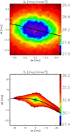 |
Fig. 6. Same symbols as Fig. 4, but for the central surface brightness. The horizontal black line denotes the observational value of 27.1. |
To find the region of the space of initial parameters that yield a model that matches the observed value, the procedure that was described in Sect. 3.1 is used. The matching points in the initial parameter space are shown in Fig. 7, where they form a tight power law that, after fitting an expression of the form Mpl = A ⋅ log10Rpl + B, leads to:
![Mathematical equation: $$ \begin{aligned} M_{\rm pl}[{M_\odot }] = 0.666_{-0.052}^{+0.056}\times R^{2.68\pm 0.01}_{\rm pl}\, [\mathrm{pc} ]. \end{aligned} $$](/articles/aa/full_html/2020/01/aa35602-19/aa35602-19-eq5.gif) (5)
(5)
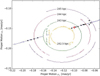 |
Fig. 7. Pairs of initial parameters which lead to final models with the correct central surface brightness of Canes Venatici I dSph. |
3.3. Effective radius
To obtain the effective radius (defined as the radius of the isophote containing half of the total luminosity) of the remnant, we used the surface brightness as a function of the projected distance to the centre of the object, and then fit a Sérsic profile to get the parameters. To construct the light profiles, we omitted the central 0.1°, which might still contain a bound object. We fitted out to 0.25°, the visible part of CVn I dSph as seen by Okamoto et al. (2012) and covering almost one kpc from the centre of the object, that is twice the effective radius measured by Martin et al. (2008b), using concentric circles to measure the light of the remnant.
The effective radius of the models at the end of the simulation are obtained via a Sérsic fit and then plotted in a double logarithmic graph (Fig. 8). From this plot we can see that for compact objects (models with low Rpl or high Mpl) we obtain lower effective radii than for more extended and easily disrupted Plummer spheres.
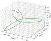 |
Fig. 8. Same symbols as Fig. 4, but for the effective radius. The horizontal black line denotes the observational value of 564 pc. |
The value for the effective radius that we need to match with these models is 564 pc (see Table 1), represented with a black horizontal line in Fig. 8. Following the same steps from the previous sections we obtain the pairs of initial values that reproduce the observable (Fig. 9) and fit the power law to get:
![Mathematical equation: $$ \begin{aligned} M_{\rm pl}[{M}_\odot ] = 0.0017_{-0.0005}^{+0.0007} \times R^{3.596\pm 0.054}_{\rm pl}\, [\mathrm{pc} ]. \end{aligned} $$](/articles/aa/full_html/2020/01/aa35602-19/aa35602-19-eq6.gif) (6)
(6)
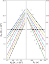 |
Fig. 9. Pairs of initial parameters which lead to final models with the correct effective radius of Canes Venatici I dSph. Despite the large error bars, the points form a tight power law, shown in Eq. (6). |
3.4. Velocity dispersion
To measure the velocity dispersion of the remnant, we use all the particles inside a region covering ±0.15° in RA and ±0.05° in DEC from the centre of the object, equivalent to the region used by Simon & Geha (2007), so we use not only the particles from the bound centre, but also the ones that form the tidal tails of the object. They report a value of 7.6 km s−1 as the velocity dispersion of CVn I dSph, and we use this as the value that has to be matched.
Following the analysis made by Blaña et al. (2015) we fit the solutions where the object is almost destroyed, that is objects with low initial masses and high Plummer radii, trying to match the velocity dispersion mentioned above. On this part of the parameter space, the central part of the remnant, still bounded, is surrounded by a large number of unbounded particles (the ones that form the tidal tails of the object and can be found at the background and foreground of the centre of the remnant).
It is the influence of these particles plus the fact that for the chosen orbit, at the end of the 10 Gyr of simulation, the remnant is close to the apocentre what boosts the velocity dispersion of the object (Smith et al. 2013a) to the observed levels, without using a DM-dominated progenitor. Smith et al. (2013a) have shown that for the required boosting of the velocity dispersion the original object has to be almost or even completely destroyed. At this stage of the evolution neither a 3−σ clipping nor the more elaborate IRT method, quoted in Klimentowski et al. (2009), are able to distinguish between bound and unbound stars and return similar results as the simple calculation used here (Smith et al. 2013a).
From Fig. 10, where the black horizontal line represents the observed value for the line-of-sight velocity dispersion, we see that increasing the mass of the model does not increase the value of this observable (left panel shows decreasing velocity dispersion with increasing mass; right panel has the fitting lines for the most massive choices lower than for less massive objects, see the colour coding and compare with previous figures), as would happen if the object is in virial equilibrium, since a more massive object prevents a larger loss of particles under the effect of the MW tides and, therefore, there are less stars in the tidal tails that would increase the value of σ. A model with larger Rpl will lose more mass and has more particles in the tidal tails, boosting the observed velocity dispersion (left panel shows fitting lines for larger initial objects higher up than for more concentrated one, compare colour coding with previous figures; right panel shows increasing velocity dispersion with increasing initial Plummer radius). Again, after fitting the power laws from Fig. 10 and obtaining the pairs of initial parameters that result in the correct velocity dispersion, we plot them (Fig. 11) and fit the corresponding power law for this observable:
![Mathematical equation: $$ \begin{aligned} M_{\rm pl}[{M}_\odot ] = 0.0014_{-0.0002}^{+0.0003} \times R^{3.645\pm 0.033}_{\rm pl}\, [\mathrm{pc} ] \end{aligned} $$](/articles/aa/full_html/2020/01/aa35602-19/aa35602-19-eq7.gif) (7)
(7)
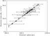 |
Fig. 10. Same symbols as Fig. 4, but for the velocity dispersion. The horizontal black line denotes the observational value of 7.6 km s−1. |
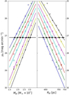 |
Fig. 11. Pairs of initial parameters which lead to final models with the correct line-of-sight velocity dispersion of Canes Venatici I dSph. |
3.5. Final model
Equations (4), (5), (6), and (7) represent the initial conditions that a Plummer sphere must have, to match each of the observables, separately. Therefore, the intersection of these lines will indicate the pair (Rpl,Mpl) that matches all the observed properties of CVn I dSph. In a ideal world, all the lines would intersect at the same point of the parameter space. In the real world, this does not happen. Nonetheless, the lines form a small region where the final model, i.e the model that, after orbiting for 10 Gyr in the orbit determined in Sect. 2, will produce a remnant whose observational parameters are within the errors of the observational data, is located. In our case, the final model should be located in the region with 600 pc ≤ Rpl ≤ 700 pc and 20.5 × 10⁶ M⊙ ≤ Mpl ≤ 30 × 106 M⊙.
The four lines are shown in Fig. 12, together with the initial parameters of the models used in this work. In the area where these four lines come close to each other, we use a trial and error approach to find the final model. A summary of the models used and the final parameters at the end of the simulation can be found in Table 5.
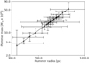 |
Fig. 12. Zone where the best fitting model for CVn I in the chosen orbit is located. Each line represents the initial parameters needed to match the four observables used on this project: Final mass (blue), central surface brightness (cyan), effective radius (red), and velocity dispersion (green). The magenta crosses are the parameters of the Plummer spheres used to calculate the power laws of Sects. 3.1, 3.2, 3.3, and 3.4. The red circle is the final model and the black stars are the rejected models. |
Initial and final parameters of the candidates for the final model.
We compare the final values of mass, surface brightness, effective radius, and velocity dispersion, plus ellipticity and position angle, of the candidates with the observed values to choose the final model. From these, the fifth model, with the pair of initial parameters Rpl = 653 pc and Mpl = 2.47 × 10⁷ M⊙, produces an object that matches the observed properties of CVn I dSph at the end of the simulation, with an infall time of 10 Gyr, with values within the observational errors: a final mass of 2.45 × 10⁵ M⊙, central surface brightness of 25.7 mag arcsec−2, effective radius of 553.8 pc, and a velocity dispersion with the value 7.61 km s−1 (see Fig. 13 and compare with Fig. 8 of Simon & Geha 2007).
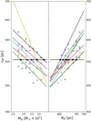 |
Fig. 13. Velocity histogram of the final object. We calculate the velocity dispersion of the remnant by selecting particles in the region covering ±0.15° in RA and ±0.05° in Dec. Compare with Fig. 8 of Simon & Geha (2007). |
A summary of the properties of the remnant can be found in Table 5 and a 2D contour plot of the object in Fig. 14. In the top panel we see that our final object has the correct elongation along the orbit, that is position angle, as well as the correct ellipticity. In the lower panel we increase the field of view (and lower the resolution as well) to show how the tidal tails align with the chosen orbit and how compressed they appear because the object is close to the apo-centre of its orbit. We point out that the colour scale is different in the top and lower panel. Furthermore, it quite clear that the far away tails shown in the lower panel have surface brightnesses far below any observational detection limit available today.
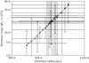 |
Fig. 14. 2D contour plot of the surface brightness of the best-matching model using a generic M/L of unity. Top panel: innermost square-degree shown with a resolution of 144 arcsec per pixel. Compare with Fig. 1. Bottom panel: 50 × 50 degrees showing the extend of the tidal tails along the orbit. The resolution is 0.5 degree. It is important to note that yellow to red contours in this panel have surface brightnesses below any normal observational detection limit. |
4. Conclusions
There are different scenarios that explain the formation and evolution of dSphs like CVn I. Some use dwarf galaxies embedded in dark halos (Mayer et al. 2007; D’Onghia et al. 2009) or dissolving star clusters inside said dark haloes (Assmann et al. 2013a,b; Alarcón Jara et al. 2018). Unlike them, and in the same vein as Blaña et al. (2015) and Domínguez et al. (2016), in this work we offer an alternative way to reproduce the characteristics of CVn I, without using DM nor any modification to the Newtonian gravity.
In the scenario we present here, we use a DM-free progenitor at the start of our simulations and explain the measured elongation of the dwarf satellite as tidal distorsions due to the disruptive forces acting on the object, that is peri-centre passages and/or disc passages. The high velocity dispersion is not caused by a massive DM halo but is the effect of many unbound stars surrounding the object mimicking a Gaussian-like distribution of velocities similar to an object in equilibrium. The actual initial object in this scenario could either be a DM-free object from the start like an extended star cluster or a tidal dwarf galaxy, or it could be a former DM dominated object which has lost all or most of its dark matter due to the tidal forces of the MW. If there were other mechanisms that played a rôle in the evolution of CVn I (e.g. close encounters with other satellites, gas loss via reionization or ram pressure stripping), then the initial mass that we present here would be a lower limit for the real initial mass of this dSph.
As we use phase-space particles instead of stars and completely neglect the contribution of any gas component in the early stages of CVn I’s history, it might be interesting for future projects to study the impact of gas stripping or stellar feedback as contributors to its evolution, mass loss, and subsequent tidal disruption by the MW. On the other hand we use a MW potential as it is seen now throughout the simulation. In reality we expect that the mass of the MW was growing during the last 10 Gyr to reach its value now. Taking this effect into account would help the survival of the initial object. Furthermore, we do neglect dynamical friction. This would place the initial object on a more distant orbit to begin with, which again would help in the survival of the satellite.
We were able to find a pair of initial parameters of a Plummer sphere that reproduces the current observational properties of CVn I dSph (Table 5). With a initial mass of 2.47 × 10⁷ M⊙ and Plummer radius of 653 pc, we obtain a remnant with a final mass of 2.45 × 10⁵ M⊙, central surface brightness of 26.9 mag arcsec−2, an effective radius of 545.7 pc, and a velocity dispersion with the value 7.58km s−1, properties that matches the observational parameters within the measurement errors.
To achieve this, first we had to find an orbit for this dwarf galaxy. Under the assumption that Canes Venatici I is a DM-free object, its elongation, as observed by Okamoto et al. (2012), would be a consequence of the tidal disruption that this galaxy is suffering under the influence of the MW’s gravitational potential and, therefore, this dwarf’s major axis would be aligned with it’s orbital path. If that weren’t the case, we could choose any other orbit, as long as the resulting object has the same radial velocity as it is observed in CVn I. Its high velocity dispersion can be explained by tidal debris surrounding the object, so the chosen orbit has to produce a high mass loss, and as long as the object is close to the apo-centre, the velocity dispersion will be boosted.
With these three points in mind, we choose a very eccentric orbit (ϵ ∼ 0.85), with a small perigalactic distance (Dp ∼ 20 kpc) and an apogalactic distance close to the current distance of CVn I dSph (Da ∼ 243 kpc, DCVnI ∼ 224 kpc). Using this orbit, we explored the space of initial parameters for the Plummer sphere, covering from 320 pc ≤ Rpl ≤ 890 pc to 4 × 10⁶ M⊙ ≤ Mpl ≤ 108 M⊙. With these results we found the power laws that represent the pairs of initial parameters that reproduce the respective observable. In the region where all the power laws come close to each other (600 pc ≤ Rpl ≤ 700 pc, 20.5 × 10⁶ M⊙ ≤ Mpl ≤ 30 × 106 M⊙), we found the final model described above, the one that manages to reproduce the current observational parameters of CVn I dSph.
This study shows, that it is possible to find a DM free progenitor, which matches all the structural and dynamical observables of Canes Venaticii I. This finding, by no means, claims to be the only possible scenario to explain this particular dwarf galaxy, but simply adds an additional possible formation and/or evolution channel, without invoking alterations to the gravity law.
Acknowledgments
DRMC, MF, AGAJ, CAA and FUZ acknowledge financial help through Fondecyt regular No. 1180291 and BASAL “Centro de Astrofisica y Tecnologias Afines” (CATA) No. AFB-170002. MF additionally acknowledges financial support through Conicyt PII20150171 and Quimal 170001. AGAJ acknowledges financial support from Carnegie Institution of Washington with its Carnegie-Chile Fellowship.
References
- Alarcón Jara, A. G., Fellhauer, M., Matus Carrillo, D. R., et al. 2018, MNRAS, 473, 5015 [NASA ADS] [CrossRef] [Google Scholar]
- Assmann, P., Fellhauer, M., Wilkinson, M. I., & Smith, R. 2013a, MNRAS, 432, 274 [NASA ADS] [CrossRef] [Google Scholar]
- Assmann, P., Fellhauer, M., Wilkinson, M. I., Smith, R., & Blaña, M. 2013b, MNRAS, 435, 2391 [NASA ADS] [CrossRef] [Google Scholar]
- Belokurov, V., Zucker, D. B., Evans, N. W., et al. 2007, ApJ, 654, 897 [NASA ADS] [CrossRef] [Google Scholar]
- Blaña, M., Fellhauer, M., Smith, R., et al. 2015, MNRAS, 446, 144 [NASA ADS] [CrossRef] [Google Scholar]
- Bournaud, F. 2010, Adv. Astron., 2010 [NASA ADS] [CrossRef] [Google Scholar]
- Bournaud, F., Duc, P.-A., & Masset, F. 2003, A&A, 411, L469 [NASA ADS] [CrossRef] [EDP Sciences] [Google Scholar]
- Bournaud, F., Bois, M., Emsellem, E., & Duc, P.-A. 2008, Astron. Nachr., 329, 1025 [NASA ADS] [CrossRef] [Google Scholar]
- Domínguez, R., Fellhauer, M., Blaña, M., et al. 2016, MNRAS, 461, 3630 [NASA ADS] [CrossRef] [Google Scholar]
- D’Onghia, E., Besla, G., Cox, T. J., & Hernquist, L. 2009, Nature, 460, 605 [NASA ADS] [CrossRef] [Google Scholar]
- Duc, P.-A. 2012, Astrophys. Space Sci. Proc., 28, 305 [NASA ADS] [CrossRef] [Google Scholar]
- Duc, P.-A., Paudel, S., McDermid, R. M., et al. 2014, MNRAS, 440, 1458 [NASA ADS] [CrossRef] [Google Scholar]
- Fellhauer, M., Kroupa, P., Baumgardt, H., et al. 2000, New Astron., 5, 305 [NASA ADS] [CrossRef] [Google Scholar]
- Fellhauer, M., Belokurov, V., Evans, N. W., et al. 2006, ApJ, 651, 167 [NASA ADS] [CrossRef] [Google Scholar]
- Fouquet, S., Hammer, F., Yang, Y., Puech, M., & Flores, H. 2012, MNRAS, 427, 1769 [NASA ADS] [CrossRef] [Google Scholar]
- Fritz, T., Battaglia, G., Pawlowski, M., et al. 2018, A&A, 619, A103 [NASA ADS] [CrossRef] [EDP Sciences] [Google Scholar]
- Hammer, F., Yang, Y., Fouquet, S., et al. 2013, MNRAS, 431, 3543 [NASA ADS] [CrossRef] [Google Scholar]
- Hernquist, L. 1990, ApJ, 356, 359 [NASA ADS] [CrossRef] [Google Scholar]
- Ibata, R. A., Lewis, G. F., Conn, A. R., et al. 2013, Nature, 493, 62 [CrossRef] [Google Scholar]
- Kaviraj, S., Darg, D., Lintott, C., Schawinski, K., & Silk, J. 2012, MNRAS, 419, 70 [NASA ADS] [CrossRef] [Google Scholar]
- Klimentowski, J., Łokas, E. L., Kazantzidis, S., et al. 2009, MNRAS, 400, 2162 [NASA ADS] [CrossRef] [Google Scholar]
- Koposov, S. E., Belokurov, V., Torrealba, G., & Evans, N. W. 2015, ApJ, 805, 130 [NASA ADS] [CrossRef] [Google Scholar]
- Martin, N. F., Coleman, M. G., De Jong, J. T. A., et al. 2008a, ApJ, 672, L13 [NASA ADS] [CrossRef] [Google Scholar]
- Martin, N. F., de Jong, J. T. A., & Rix, H.-W. 2008b, ApJ, 684, 1075 [NASA ADS] [CrossRef] [Google Scholar]
- Mateo, M. L. 1998, ARA&A, 36, 435 [NASA ADS] [CrossRef] [Google Scholar]
- Mayer, L., Kazantzidis, S., Mastropietro, C., & Wadsley, J. 2007, Nature, 445, 738 [NASA ADS] [CrossRef] [PubMed] [Google Scholar]
- McConnachie, A. W. 2012, AJ, 144, 4 [NASA ADS] [CrossRef] [Google Scholar]
- Metz, M., & Kroupa, P. 2007, MNRAS, 376, 387 [NASA ADS] [CrossRef] [Google Scholar]
- Miyamoto, M., & Nagai, R. 1975, PASJ, 27, 533 [NASA ADS] [Google Scholar]
- Mizutani, A., Chiba, M., & Sakamoto, T. 2003, ApJ, 589, L89 [NASA ADS] [CrossRef] [Google Scholar]
- Muñoz, R. R., Majewski, S. R., & Johnston, K. V. 2008, ApJ, 679, 346 [NASA ADS] [CrossRef] [Google Scholar]
- Newton, O., Cautun, M., Jenkins, A., Frenk, C. S., & Helly, J. 2018, MNRAS, 479, 2853 [NASA ADS] [CrossRef] [Google Scholar]
- Okamoto, S., Arimoto, N., Yamada, Y., & Onodera, M. 2012, ApJ, 744, 96 [NASA ADS] [CrossRef] [Google Scholar]
- Pawlowski, M. S., Kroupa, P., & de Boer, K. S. 2011, A&A, 532, A118 [NASA ADS] [CrossRef] [EDP Sciences] [Google Scholar]
- Pawlowski, M. S., Pflamm-Altenburg, J., & Kroupa, P. 2012, MNRAS, 423, 1109 [NASA ADS] [CrossRef] [Google Scholar]
- Ploeckinger, S., Hensler, G., Recchi, S., Mitchell, N., & Kroupa, P. 2014, MNRAS, 437, 3980 [NASA ADS] [CrossRef] [Google Scholar]
- Ploeckinger, S., Sharma, K., Schaye, J., et al. 2018, MNRAS, 474, 580 [NASA ADS] [CrossRef] [Google Scholar]
- Plummer, H. C. 1911, MNRAS, 71, 460 [CrossRef] [Google Scholar]
- Read, J. I., Wilkinson, M. I., Evans, N. W., Gilmore, G., & Kleyna, J. T. 2006, MNRAS, 367, 387 [NASA ADS] [CrossRef] [Google Scholar]
- Recchi, S., Theis, C., Kroupa, P., & Hensler, G. 2007, A&A, 470, L5 [NASA ADS] [CrossRef] [EDP Sciences] [Google Scholar]
- Sawa, T., & Fujimoto, M. 2005, PSAJ, 57, 429 [Google Scholar]
- Scott, T. C., Lagos, P., Ramya, S., et al. 2018, MNRAS, 475, 1148 [NASA ADS] [CrossRef] [Google Scholar]
- Simon, J. D., & Geha, M. 2007, ApJ, 670, 313 [NASA ADS] [CrossRef] [Google Scholar]
- Smith, R., Fellhauer, M., Candlish, G. N., et al. 2013a, MNRAS, 433, 2529 [NASA ADS] [CrossRef] [Google Scholar]
- Smith, R., Sánchez-Janssen, R., Fellhauer, M., et al. 2013b, MNRAS, 429, 1066 [NASA ADS] [CrossRef] [Google Scholar]
- Tollerud, E. J., Bullock, J. S., Strigari, L. E., & Willman, B. 2008, ApJ, 688, 277 [NASA ADS] [CrossRef] [Google Scholar]
- Wetzstein, M., Naab, T., & Burkert, A. 2007, MNRAS, 375, 805 [NASA ADS] [CrossRef] [Google Scholar]
- Zucker, D. B., Belokurov, V., Evans, N. W., et al. 2006, ApJ, 643, L103 [NASA ADS] [CrossRef] [Google Scholar]
Appendix A: Search method for the orbits
The search method goes as follows:
-
The search area is defined as the zone in parameter space with proper motions with (μδ, c − R) ≤ μδ ≤ (μδ, c + R) and (μα, c − R) ≤ μα ≤ (μα, c + R), where R is the search radius.
-
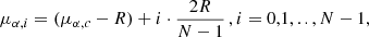
The search area is divided in N2, equally spaced, pairs of proper motions (μα, i, μδ, j), where:
 (8)
(8) (9)
(9) -
For each of these pairs of proper motions, the orbit is calculated using a simple point mass integrator.
-
This orbit is projected on the sky and its position angle measured at the current coordinates of CVn I.
-
The difference ΔPA between CVn I’s position angle and the projected orbit’s inclination (see Fig. 1) is calculated.
-
The N pairs (μα, i, μδ, i) that gave values with 0 ≤ ΔPA < 5 are saved (since these are the orbits that closely match the position angle of CVn I dSph) and the rest are discarded.
-
For each of these N pairs (μα, i, μδ, i), this process is repeated, now with:

To find the candidates using this method, the initial values chosen were:

The value of N can be increased if we needed more resolution or faster results, but N = 7 is a good compromise, so at the end the 343 orbits showed us the region on parameter space where the orbit has the same inclination as the observed object.
The technique described is flexible enough to use other properties of the orbit to select regions of this space, like perigalactic or apogalactic distance. Since CVn I dSph has a high velocity dispersion, the chosen orbit should be the one that will give the highest boost on this value of the final object.
All Tables
All Figures
|
Fig. 1. Projected orbit of CVn I dSph on the sky. The red dashed line represents the past position of CVn I dSph, while the green line corresponds to the future position of the galaxy. The blue dots are aligned to the major axis of the dwarf. The isodensity contour plot was adapted from Okamoto et al. (2012), Fig. 8. |
| In the text | |
|
Fig. 2. Proper motions of the orbit candidates. The blue dots represent the pairs of proper motions that match the position angle of CVn I, while the purple, red, green, and yellow dotted circles mark the zone of parameter space where the orbits have apogalactic distances of 245 kpc, 244 kpc, 243 kpc, and 242.5 kpc, respectively. The black crosses are the candidates for the final orbit (Table 2), while the red plus sign is the selected orbit. |
| In the text | |
|
Fig. 3. Selected orbit for CVn I. The green line shows the position of the point mass particle backwards in time, the blue square the position at t = −10 Gyr and the red triangle the current position of CVn I. Axes centred on the Galactic centre. |
| In the text | |
|
Fig. 4. Final mass as a function of the initial parameters of the model. Left: final mass as a function of the initial mass. Shown here are the data points and fitting lines for Plummer radii of 560 (blue dots), 610 (green triangles), 660 (red squares), 710 (cyan diamonds), 760 (magenta stars), 830 (yellow circles), and 890 pc (black triangles). Right: final mass as a function of the Plummer radius. Shown here are the data point and fitting lines for Plummer masses of 17.37 × 10⁶ (blue circles), 19.2 × 10⁶ (green triangles), 21.21 × 10⁶ (red squares), 23.44 × 10⁶ (cyan diamonds), 25.9 × 10⁶ (magenta stars), 28.61 × 10⁶ (yellow circles), and 31.62 × 10⁶ M⊙ (black triangles). Horizontal solid line denotes the adopted value of the final mass that needs to be matched. The black squares are the matching values calculated by fitting power laws to the data points. |
| In the text | |
|
Fig. 5. Pairs of initial parameters which lead to final models with the correct mass of Canes Venatici I dSph. |
| In the text | |
|
Fig. 6. Same symbols as Fig. 4, but for the central surface brightness. The horizontal black line denotes the observational value of 27.1. |
| In the text | |
|
Fig. 7. Pairs of initial parameters which lead to final models with the correct central surface brightness of Canes Venatici I dSph. |
| In the text | |
|
Fig. 8. Same symbols as Fig. 4, but for the effective radius. The horizontal black line denotes the observational value of 564 pc. |
| In the text | |
|
Fig. 9. Pairs of initial parameters which lead to final models with the correct effective radius of Canes Venatici I dSph. Despite the large error bars, the points form a tight power law, shown in Eq. (6). |
| In the text | |
|
Fig. 10. Same symbols as Fig. 4, but for the velocity dispersion. The horizontal black line denotes the observational value of 7.6 km s−1. |
| In the text | |
|
Fig. 11. Pairs of initial parameters which lead to final models with the correct line-of-sight velocity dispersion of Canes Venatici I dSph. |
| In the text | |
|
Fig. 12. Zone where the best fitting model for CVn I in the chosen orbit is located. Each line represents the initial parameters needed to match the four observables used on this project: Final mass (blue), central surface brightness (cyan), effective radius (red), and velocity dispersion (green). The magenta crosses are the parameters of the Plummer spheres used to calculate the power laws of Sects. 3.1, 3.2, 3.3, and 3.4. The red circle is the final model and the black stars are the rejected models. |
| In the text | |
|
Fig. 13. Velocity histogram of the final object. We calculate the velocity dispersion of the remnant by selecting particles in the region covering ±0.15° in RA and ±0.05° in Dec. Compare with Fig. 8 of Simon & Geha (2007). |
| In the text | |
|
Fig. 14. 2D contour plot of the surface brightness of the best-matching model using a generic M/L of unity. Top panel: innermost square-degree shown with a resolution of 144 arcsec per pixel. Compare with Fig. 1. Bottom panel: 50 × 50 degrees showing the extend of the tidal tails along the orbit. The resolution is 0.5 degree. It is important to note that yellow to red contours in this panel have surface brightnesses below any normal observational detection limit. |
| In the text | |
Current usage metrics show cumulative count of Article Views (full-text article views including HTML views, PDF and ePub downloads, according to the available data) and Abstracts Views on Vision4Press platform.
Data correspond to usage on the plateform after 2015. The current usage metrics is available 48-96 hours after online publication and is updated daily on week days.
Initial download of the metrics may take a while.