| Issue |
A&A
Volume 632, December 2019
|
|
|---|---|---|
| Article Number | A70 | |
| Number of page(s) | 7 | |
| Section | Planets and planetary systems | |
| DOI | https://doi.org/10.1051/0004-6361/201936378 | |
| Published online | 02 December 2019 | |
Thermal evolution of Uranus and Neptune
I. Adiabatic models
1
Institut für Physik, Universität Rostock,
A.-Einstein-Str. 23,
18059 Rostock,
Germany
e-mail: This email address is being protected from spambots. You need JavaScript enabled to view it.
2
Institut für Planetenforschung, Deutsches Zentrum für Luft- und Raumfahrt,
Rutherfordstraße 2,
12489 Berlin,
Germany
Received:
25
July
2019
Accepted:
22
October
2019
Abstract
The brightness of Neptune is often found to be in accordance with an adiabatic interior, while the low luminosity of Uranus challenges this assumption. Here we apply revised equation of state data of hydrogen, helium, and water and compute the thermal evolution of Uranus and Neptune assuming an adiabatic interior. For this purpose, we have developed a new planetary model and evolution code. We investigate the influence of albedo, solar energy influx, and equations of state of H and He, and water on the cooling time. Our cooling times of about τU = 5.1 × 10⁹ yr for Uranus and τN = 3.7 × 10⁹ yr for Neptune bracket the known age of the planets of 4.56 × 10⁹ yr implying that neither planet’s present-day luminosity can be explained by adiabatic cooling. We also find that uncertainties on input parameters such as the level of irradiation matter generally more for Uranus than for Neptune. Our results suggest that in contrast to common assumptions, neither planet is fully adiabatic in the deeper interior.
Key words: planets and satellites: physical evolution / planets and satellites: interiors / planets and satellites: individual: Uranus / planets and satellites: individual: Neptune
© ESO 2019
1 Introduction
Uranus and Neptune, the two outermost planets of our solar system, share a large number of very similar observed values such as mean density, surface temperature, atmospheric composition, and magnetic field morphology (Guillot & Gautier 2015). These observations suggest similar structural and evolutionary paths since their time of formation 4.56 × 10⁹ yr ago. Because of their similar characteristics, which are different from the larger primarily hydrogen- and helium-based gas giants Jupiter and Saturn and the smaller rock-based inner planets, they are usually classified in their own category as ice giants.
Neptune’s intrinsic heat flux of Fint, N = 0.433 ± 0.046 Wm−2 is about an order of magnitude higher than that of Uranus (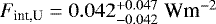 ) (Guillot & Gautier 2015). Uranus’ intrinsic flux is consistent with being zero, meaning that it could be in thermal equilibrium with the Sun, while Neptune is clearly still cooling.
Earlier adiabatic cooling calculations using a zero-temp- erature equation of state (EOS) for the ice material have found that both planets are cooling too slowly to explain their present-day luminosity (Hubbard 1978; Hubbard & McFarlane 1980; Hubbard et al. 1995). More recent models, using a finite-temperature EOS for water but currently outdated ones for hydrogen and helium, could reproduce Neptune’s brightness but still obtained too high luminosity for Uranus (Fortney et al. 2011; Nettelmann et al. 2013; Linder et al. 2019).
It is important to gain better insight into the thermal structure of Uranus and Neptune and their heat fluxes because the thermal structure largely influences the inferred composition (Podolak et al. 2019). As of June 2019, out of the 3972 confirmed and categorised exoplanets1, more than 30% are in a size range similar to Neptune and about 30% are intermediate in size between Earth and Neptune. Due to selection effects in exoplanet surveys, however, these numbers refer to the detected planets, while the absolute occurrence rates at large orbital distances (>100 days) are not known yet. Nevertheless, understanding Uranus and Neptune is an important step towards understanding a frequently occurring class of exoplanets.
In this work, we apply the Rostock Equation of State version 3 (Becker et al. 2014, REOS.3) for hydrogen and helium and the recently published water EOS by Mazevet et al. (2019) to calculate new adiabatic cooling times for Uranus and Neptune. We investigate the influence of solar energy influx and EOS data on the cooling behaviour. To this end, we present the theoretical foundations of a newly developed computer code in Sect. 2 and calculate a variety of planetary cooling tracks with different assumptions. The results are presented and discussed in Sect. 3. Section 4 summarises the results and gives a brief outlook.
2 Methodology
2.1 Theoretical foundations
To compute the thermal evolution of fluid planets we developed a new tool, which we named OTher Thermal Evolution Realisation (OTTER). It is based on the following basic equations, representing conservation of mass, hydrostatic equilibrium, energy transport, and conservation of energy for the main variables of radius r(m), pressure P(m), temperature T(m), and luminosity l(m) (Kippenhahn et al. 2012):
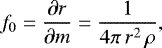 (1)
(1)
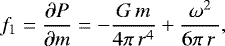 (2)
(2)
 (3)
(3)
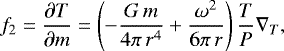
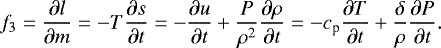 (4)
(4)
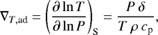
Equations (2) and (3) contain terms arising from rigid body rotation in zeroth order. In Eq. (3),  denotes the temperature gradient that is evaluated at each point separately. In this work we follow the commonly used assumption of a convective adiabatic interior for gas and ice giants (Guillot 1999; Helled et al. 2011), which means for ∇T we use the adiabatic gradient (Kippenhahn et al. 2012)
 (5)
(5)
where  is the thermal expansion coefficient and
  the isobaric heat capacity. The two outer boundary conditions at m = MP are
 (6)
(6)
 (7)
(7)
where σB = 5.6704 × 10⁻⁸ Wm−2 K−4 is the Stefan–Boltzmann constant, Lsol the solar radiation absorbed and re-emitted by the planet, and Teff denotes the planet’s effective temperature. We link it to the one-bar temperature via
 (8)
(8)
Equation (8) is based on model atmospheres for Jupiter developed by Graboske et al. (1975) and interpolated by Hubbard (1977). The parameter K is chosen to yield the present-day one-bar temperatures for Uranus and Neptune for their present-day radius and effective temperature. We find KU = 1.481 for T1 bar = 76 K for Uranus and KN = 1.451 for T1 bar = 72 K for Neptune. Compared to the model atmosphere by Fortney et al. (2011) developed for Uranus and Neptune, we find that K changes only by a small percent with Teff and g except for high values of Teff, where the cooling time is short. We therefore assume it to be constant over the planet’s lifetime.
Following Kippenhahn et al. (2012), we define four functions  at the jth point of a mass grid for a given time
 (9)
(9)
Here yi are the logarithmic main variables y0 = ln(r), y1 = ln(P), y2 = ln(T), y3 = ln(l); the values  are obtained as the arithmetic mean of the values at the jth and (j + 1)st point. The functions fi are the derivatives of the main variables as defined in Eqs. (1)–(4). We use
 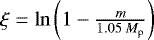 as our mass coordinate, following Kippenhahn et al. (1967). Approximating the derivatives as the corresponding difference coefficient, a profile that fulfils Eqs. (1)–(4) must satisfy
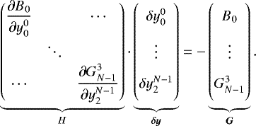
  . Similarly, the two outer boundary conditions (6) and (7) are formulated as B0 and B1. Therefore, for N mass points, we have a system of 4N − 2 equations. Using Newton’s method, it can be solved by recasting to the matrix equation
 (10)
(10)
For a given time, the matrix H and the vector G are constructed using an estimated solution. Solving the equation above then yields corrections  for every main variable at every mass point, which are added to the estimate to generate a new input. This is repeated until all the corrections fulfil the truncation condition
  , which means the profile is converged. The difference between using this condition in comparison to
  lies in the tenth digit of the effective cooling time. Then, a new estimated solution for the next time step is estimated based on the current and the previous time step, and a new profile is calculated for the new time.
The planet’s rotation period is fixed over the whole evolution time at tω,U = 6.206 × 10⁴ s for Uranus and tω,N = 5.8 × 10⁴ s for Neptune (Guillot & Gautier 2015). Accounting for angular momentum conservation leads to a change in rotational period of about ten hours over the course of the planet’s evolution; however, we found only a small effect on the resulting cooling times and therefore neglect it for numerical simplicity. The program is coded in C++ and uses sparse matrix functions from the Eigen-library (Guennebaud et al. 2010) to solve the relevant matrix equations.
2.2 Equations of state
Uranus and Neptune are commonly assumed to be composed primarily of conducting fluid ices as well as hydrogen and helium (Podolak et al. 1995).
In this paper we apply four different EOSs for hydrogen and helium. For benchmark purposes, in Sect. 2.3 we use the SCvH H/He EOS (Saumon et al. 1995), while in Sect. 3, for our adiabatic Uranus and Neptune models, we apply the two versions of the Rostock EOS, REOS.1 (Nettelmann et al. 2008) and REOS.3 (Becker et al. 2014), and the recent EOS by Chabrier et al. (2019).
In H-REOS.3, the DFT-MD data are based on simulations using 256 particles (H-REOS.1: 64 particles). In H-REOS.3, the internal energy is corrected for the quantum mechanical energy of harmonic oscillations of the H2 molecule, while H-REOS.1 only accounts for the classical treatment of the vibrations. These two changes were already applied to H-REOS.2 (Nettelmann et al. 2012); however, that EOS was built on a coarser temperature grid at low temperatures subject to larger uncertainties upon interpolation.
He-REOS.3 differs from He-REOS.1 in that it is based on DFT-MD data using 108 particles (He-REOS: 32-64) on a significantly denser temperature grid than He-REOS.1. Moreover, the DFT-MD data in He-REOS.3 are connected to virial EOS data at T − ρ conditions relevant to planets, namely at ρ < 0.1 g cm−3 and T < 1 × 10⁴ K, while at high temperatures more relevant to hot Jupiters and brown dwarfs it connects to the He-SCvH EOS. Instead, He-REOS.1 exclusively connects to Sesame EOS 5761 at low densities and/or high temperatures.
The EOS by Chabrier et al. (2019; hereafter Chabrier-EOS) uses the SCvH data in the low-temperature and low-pressure regime. At high temperatures and high pressures, where the material is fully ionised, it utilises data from Chabrier & Potekhin (1998). In the intermediate regime of partial ionisation and dissociation, the Chabrier-EOS employs results of quantum molecular dynamics calculations. The different data sets are combined via a bicubic spline interpolation. Like the SCvH data, this EOS provides the entropy and adiabatic temperature gradient explicitly. Since it does not extend to T < 100 K, models featuring this EOS use REOS.3-data for H and He for low temperatures.
In the representation of ices, here we use EOSs of pure water as in Helled et al. (2011) and Nettelmann et al. (2013). This is certainly a simplification since the further ice-forming elements carbon, nitrogen, and sulphur are likely to be present in the interior as well. Former work has shown that the presence of ices lighter than water in solar element ratios can lead to the extreme case of an icy inner envelope (Podolak & Reynolds 1987) and hence a cooler planet (Bethkenhagen et al. 2017). On the other hand, rocks may be soluble in hydrogen and thus be present to some degree in the envelope at the expense of ices, while methane may be insoluble in water and may lead to carbon sedimentation. Given these uncertainties on the deep interior composition, we believe that the uncertainty added by our simplification does not change the conclusions of this work.
We consider two water equations of state. The Sesame 7150 EOS (Ree 1976) is a combination of experimental work and chemical model data connected via interpolation, which makes it quite accurate for lower temperatures but less so for the warm dense interior of the ice giants where there are few experimental results (see Knudson et al. 2012 for a comparison of water EOS data along the principal Hugoniot). Recently, a new water EOS was released by Mazevet et al. (2019). It is based on a thermodynamically consistent Helmholtz free energy parameterisation over a wide range of temperature-pressure conditions and incorporates EOS data from various sources, including ab initio simulation data. In order to handle the low-temperature phase transitions between solid, liquid, and gaseous water below the critical point, we applied a Maxwell construction on the water EOS of Mazevet et al. (2019), in the following labelled “Mazevet EOS”. However, due to numerical difficulties in handling first-order phase transition, we use an ideal gas description for water for T < 800 K, independently of whether the Sesame-EOS or Mazevet-EOS is used for the majority of the planet. This ideal gas description contains quantum mechanical corrections of the vibrational and rotational energy of the H2 O-molecule following French & Redmer (2009).
The different EOS data of different materials are combined via the linear mixing rule, ρ−1 = ∑iXi∕ρi and u = ∑iXiui, where Xi are the different species’ mass fractions, which is a reasonable assumption, as shown by Bethkenhagen et al. (2017). The rock core is represented by the Sesame 7530 EOS for basalt (Lyon & Johnson 1992).
2.3 Benchmarking with respect to MOGROP
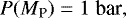
To verify the results provided by our new code, we compared our evolution curves obtained with OTTER to evolution curves using the MOGROP code (Nettelmann et al. 2012). For this purpose, a test planet of MP = 300 ME with a small rock core and an adiabatic hydrogen envelope was considered.
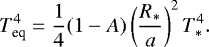
Figure 1 shows that both codes produce similar thermal evolution tracks if the hydrogen EOS by Saumon et al. (1995) is used for the envelope, which provides explicitly the adiabatic temperature gradient and the entropy. However, when using the H-REOS.3 hydrogen EOS table (Becker et al. 2014), which does not include these quantities, the level of agreement depends on the method of calculating the luminosity. Using MOGROP’s standard way of calculating the heat, which draws on the planet’s entropy profile calculated via thermodynamic integration from internal energy and density, we find a large difference from OTTER’s evolution curve (compare the black solid and the green dot-dashed curves in Fig. 1). However, using interior energy and density directly instead of entropy in MOGROP (cf. Eq. (4)), we find good agreement with the new code (compare the black dashed and the red dot-dashed curves in Fig. 1). As the ultimate reason for this behaviour, we identify imperfect thermodynamic consistency in the H-REOS-table which leads to amplified uncertainties on the entropy, which in the MOGROP code is derived by thermodynamic integration on the EOS data u(T, ρ), P(T, ρ) (see Nettelmann et al. 2012). The uncertainties on the heat δQ are apparently much smaller when simply interpolating in these data directly.
These findings suggest that there may be larger uncertainties on previous evolution calculations than assumed. It also emphasises the need for wide-range thermodynamically consistent EOSs in planetary modelling for the most abundant materials H, He, and H2O.
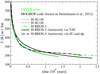 |
Fig. 1 Evolution of a 300 ME planet with a 2 ME rock core and an adiabatic hydrogen envelope. Shown are comparisons between the OTTER code (red, this work) and the MOGROP code (black, Nettelmann et al. 2012) for two different hydrogen equations of state–thin: SCvH-EOS (Saumon et al. 1995); thick: REOS.3 (Becker et al. 2014)–and, for MOGROP, different ways of calculating the luminosity. |
3 Results
3.1 Interior models
Below we present our results for interior models and thermal evolution curves for Uranus and Neptune. The models employ an adiabatic temperature profile and are separated into a hydrogen- and helium-rich outer envelope with a certain amount of water as a representation of heavy elements, a water-rich inner envelope with only a small fraction of hydrogen and helium, and a small isothermal rock core. It has been shown by Linder et al. (2019) that there is little difference in luminosity between an isothermal and an adiabatic rock core. The structure models have a discontinuity in composition at about 30 GPa between the outer and inner envelope. Table 1 shows the parameters of the structure models, which were chosen to reproduce the planet’s present day mean radius. For each planet there are two structure models, one using the Sesame 7150 EOS for water (Ree 1976), the other using the EOS by Mazevet et al. (2019) (see Sect. 2.2 for details).
The total mass of hydrogen and helium also given in the table is consistent with values of previously published models that satisfy the gravity data (Helled et al. 2019). However, hydrogen and helium in our models are more concentrated towards the surface. Consequently, the gravitational moments J2, J4 are lower than the measured values (cf. Nettelmann et al. 2013) by about ~ 20 % for Uranus and ~5% for Neptune. Due to the sensitivity of Uranus’ cooling times to small changes in the assumptions (see Sect. 3.4 for details), this could lead to a shift in Uranus’ effective cooling time of up to 1 Gyr. However, the systematic behaviour with the parameters studied here remains unaffected by this.
In the following segments, we investigate the effect of different factors on the cooling behaviour of adiabatic Uranus and Neptune. In all figures corresponding to the various evolution calculations, the curves are shifted to run through the present-day Teff for t = 4.56 × 10⁹ yr, the age of the solar system, to allow for an easy comparison of the differences in cooling times at first glance.
3.2 Influence of hydrogen and helium equation of state
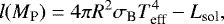
While Uranus and Neptune are thought to be composed primarily of higher density ices like water, ammonia, and methane, their gravitational moments cannot be reproduced without the presence of the lighter elements hydrogen and helium (Hubbard & McFarlane 1980; Podolak & Reynolds 1987; Helled et al. 2011; Podolak et al. 2019; Nettelmann et al. 2013). In Fig. 2 we investigate the influence of the H/He EOS (for details, see Sect. 2.2). We find that using the REOS.3 table for H and He yields a shortening of cooling times for Neptune by at least 0.6 Gyr compared to previous work. The exact amount depends somewhat on the evolution code used and on the water EOS (see Sect. 3.3). Nevertheless, the shortening is visible with both MOGROP and OTTER and seems to be caused by the different H/He EOS. Using the Chabrier-EOS for H/He leads to a further shortening of Neptune’s cooling time by about 0.5 Gyr, underscoring the importance of H and He for the cooling behaviour. Since previous work based on H/He-REOS.1 (Fortney et al. 2011; Nettelmann et al. 2013) or the Saumon et al. (1995) data (Linder et al. 2019) did reproduce the age of ~ 4.6 Gyr, the shortening found here implies that Neptune seems to be incompatible with the known age of the solar system and appears to be brighter than predicted by adiabatic cooling. As is shown in Sects. 3.3 and 3.4, with the same set of assumptions the luminosity of Uranus is also not able to be reproduced.
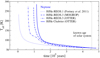 |
Fig. 2 Evolution calculations for Neptune using different H/He EOS data and codes: dotted: H/He-REOS.1, MOGROP (adapted from Fortney et al. 2011); dashed: H/He-REOS.3, MOGROP; dash-dotted: H/He-REOS.3, OTTER; solid: H/He-Chabrier, OTTER. All curves use Teq = const. (see Sect. 3.4). |
3.3 Water equation of state
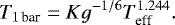
In Fig. 3 we compare adiabatic P−T relations using the Mazevet EOS and the Sesame EOS for water. These curves are taken from the structure models introduced in Table 1. For pressures larger than a few GPa, there are noticeable differences between the two models. Nevertheless, the two planets end up with similar values for the central temperature independently of water EOS, leading to a core temperature of about Tc ≈ 5700 K for Uranus and Tc ≈ 5500 K for Neptune.
Although it is cooler, the Mazevet-EOS based adiabats require a larger ice mass fraction to match the planet radius (see Table 1). A greater heavy element content, or a smaller H/He mass fraction, typically reduces the energy budget of a planet and shortens the cooling time, see Fig. 4, where using the Mazevet EOS instead of Sesame leads to a further shortening of the cooling times by about ~ 5%. The cooling curves using Sesame also feature an edge at Teff~120 K not seen in the Mazevet curves. This is caused by the behaviour of the individual adiabats’ in the deep interior of the planets at conditions of about 100 GPa and 5000 –7000K and by the differences of the EOS in that regime. However, the effect on cooling time, while noticeable, is far less than that of other influences investigated here, such as H/He EOS or solar influx. Crucially, using the Mazevet EOS also produces cooling times that are too short for Neptune and too long for Uranus.
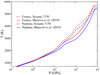 |
Fig. 3 Deep interior of Uranus (red) and Neptune (blue) with the heavy elements in the envelope treated via the Sesame water EOS (dashed) or the Mazevet EOS (solid), respectively. |
3.4 Influence of solar irradiation
An important part in calculating the evolution of a planet is the treatment of external energy being deposited into it. In our model this is expressed via the luminosity boundary condition Eq. (7), specifically the quantity of the absorbed and re-emitted solar luminosity Lsol. It can be expressed as
 (11)
(11)
with the equilibrium temperature
 (12)
(12)
Here R* denotes the Sun’s radius, T* its effective temperature, a the planet’s semi-major axis, and A its Bond albedo. All our calculations assume the latter two parameters to be fixed over the planet’s evolution.
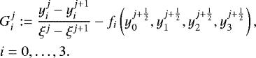
We consider three cases: Teq = 0, Teq = const., and Teq (t), which accounts for the linear increase in the Sun’s luminosity over time. Although the equilibrium temperatures of Uranus and Neptune are quite small with Teq,U = 58.1 ± 1.1 K and Teq, N = 46.4 ± 1.1 K (Guillot 2005), Fig. 4 shows a considerable influence on calculated cooling time. Entirely neglecting the solar irradiation (Teq = 0) produces very short cooling times for both Uranus and Neptune. Notably, in this case Uranus cools more quickly than Neptune. Fixing the Sun’s luminosity to its present-day value over the entire evolution (Teq = const.), as was done by Fortney et al. (2011) or Nettelmann et al. (2013), among others, gives significantly longer cooling times by about 1 × 10⁹ yr for Neptune and several billion years for Uranus. Cooling times for Teq(t), which is the most realistic case, fall between these extremes.
The differences found when using the three approaches are vastly more pronounced for Uranus than for Neptune. This is due to the fact that Uranus’ present-day effective temperature Teff = 59.1 ± 0.3 K (Guillot 2005) is very close to its equilibrium value, while Neptune is further away from that equilibrium with Teff = 59.3 ± 0.8 K (Guillot 2005). The slope of the cooling curve becomes very shallow as the planet approaches equilibrium, meaning that small changes in how that equilibrium is treated affect Uranus more than Neptune. This means that modifying assumptions such as the heavy element distribution or the spherical approximation have a stronger impact on Uranus than on Neptune so that cooling times presented here for Uranus have a rather large uncertainty. In addition, we find that the observational error bars of Teff induce an additional uncertainty of about ~0.5 Gyr for Uranus and ~0.3 Gyr for Neptune assuming adiabatic cooling.
The importance of an accurate observational grip on the solar influx can also be seen in Fig. 5 where we plot the cooling time as a function ofBond albedo A. As before, we see a more drastic influence on Uranus’ cooling than on Neptune’s. In particular, a change in Uranus’ albedo from 0.3 to 0.4 would bring its cooling time into agreement with the age of the solar system. For Neptune, however, the cooling time is shorter than the known age for all values of A. We evaluatethis as further evidence that the brightness of Neptune is inconsistent with a fully adiabatic interior.
4 Conclusions
We have presented homogeneous thermal evolution calculations for Uranus and Neptune and have investigated the impact of solar energy influx, Bondalbedo, and equations of state of hydrogen, helium, and water on the cooling behaviour. Our preferred models using REOS.3 EOSs for H and He and Mazevet et al. (2019) for water, as well as time-dependent solar luminosity predict a cooling time of about τU = 5.1 Gyr for Uranus and τN = 3.7 Gyr for Neptune. This is notably shorter than previous results and means that neither planet’s present-day luminosity can be explained by adiabatic models. Our results therefore confirm that a more sophisticated approach is required than the fully adiabatic assumption. A non-adiabatic deep interior region has been suggested by Hubbard et al. (1995) to explain the faintness of Uranus, and could also explain the magnetic field morphology of the ice giants (Stanley & Bloxham 2004, 2006); the assumption of a sharp temperature gradient at a layer boundary within Uranus’ envelope was shown by Nettelmann et al. (2016) to be able to reproduce Uranus’ correct age while also being compatible with gravitational field measurements. Moreover, physical processes like sedimentation or upwelling of a major constituent in the HCNO system could also have a large influence on the thermal evolution of the ice giants. For instance, it is possible, that demixing of hydrogen and water occurs at conditions relevant for the ice giant envelope (Bali et al. 2013), although ab initio simulations suggest solubility of water and hydrogen under Uranus and Neptune interior conditions (Soubiran & Militzer 2015). Deeper in the interior at pressures of about 1.5 Mbar, carbon-hydrates have been experimentally found to separate into diamond, which may sink to the core, and hydrogen, which may rise upward (Kraus et al. 2017). In the same vein, while first-principle calculations of 1:1 water-ammonia mixtures have suggested the presence of a stable superionic phase of H2 O and NH3 (Bethkenhagen et al. 2015), additional crystal structure searches have revealed that ammonia, when mixed with water in solar proportions, may preferentially connect to protons donated by a superionic H2 O-ice lattice and thus perhaps form an ocean of light ices on top of the water-rich deep interior (Robinson et al. 2017). Such a layercould lead to stable stratification across the region identified as a layer boundary in conventional three-layer structure models. All these processes can have a strong impact on the planetary structure and thermal evolution.
Additionally, uncertainties on the solar flux due to the present Bond albedo, which we assume to be constant over time, can have considerable influence on the planet’s cooling behaviour, which is especially pronounced for Uranus, because it is very close to being in thermal equilibrium with the Sun. This is problematic because the current albedo values of the ice giants have relatively large observational uncertainties, which could even be larger than the currently accepted error bars. We note that Cassini observations of the Jovian atmosphere recently led to a significantly higher Bond Albedo of 0.50 compared to the Voyager value of 0.34 (Li et al. 2018).
Improved observational constraints on the present values of albedo and effective temperature are thus clearly much needed also for the ice giants. Observational constraints for earlier times when the atmosphere was warmer will have to wait for albedo measurements of Neptune-like exoplanets around young Sun-like stars.
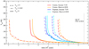 |
Fig. 4 Thermal evolution of Uranus (red and orange) and Neptune (blue and cyan). Dashed lines represent no solar incident flux, dot-dashed constant solar irradiation, and solid lines linearly changing solar luminosity (see Sect. 3.4). Also shown are two different EOSs for the water in the envelope, SESAME 7150 (Ree 1976) and Mazevet et al. (2019). |
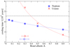 |
Fig. 5 Cooling times of Uranus and Neptune for different values of the Bond albedo. All calculations shown use Sesame EOS 7150 for water and assume a linearly changing solar luminosity with time. Diamonds indicate the observed Voyager values of A (Pearl et al. 1990; Pearl & Conrath 1991). The thin dashed lines show the hyperbolic curve fit as a guide to the eye. |
Acknowledgements
We thank the referee for helpful comments for this publication. We thank Martin French for his help in adapting the Mazevet EOS for our use, in particular for applying the Maxwell construction, and for providing fruitful discussion of the results. This project was funded by the German Research Foundation DFG as part of the Research Group FOR-2440 “Matter Under Planetary Interior Conditions”. We also acknowledge the hospitality of the International Space Science Institute in Bern.
References
- Bali, E., Audetat, A., & Keppler, H. 2013, Nature, 495, 220 [NASA ADS] [CrossRef] [Google Scholar]
- Becker, A., Lorenzen, W., Fortney, J. J., et al. 2014, ApJS, 215, 21 [NASA ADS] [CrossRef] [Google Scholar]
- Bethkenhagen, M., Cebulla, D., Redmer, R., & Hamel, S. 2015, J. Phys. Chem. A, 119, 10582 [CrossRef] [Google Scholar]
- Bethkenhagen, M., Meyer, E. R., Hamel, S., et al. 2017, ApJ, 848, 67 [NASA ADS] [CrossRef] [Google Scholar]
- Chabrier, G., & Potekhin, A. Y. 1998, Phys. Rev. E, 58, 4941 [NASA ADS] [CrossRef] [Google Scholar]
- Chabrier, G., Mazevet, S., & Soubiran, F. 2019, ApJ, 872, 51 [NASA ADS] [CrossRef] [Google Scholar]
- Fortney, J. J., Ikoma, M., Nettelmann, N., Guillot, T., & Marley, M. S. 2011, ApJ, 729, 32 [NASA ADS] [CrossRef] [Google Scholar]
- French, M., & Redmer, R. 2009, J. Phys. Condens. Matter., 21, 375101 [CrossRef] [Google Scholar]
- Graboske, H. C., Pollack, J. B., Grossman, A. S., & Olness, R. J. 1975, ApJ, 199, 265 [NASA ADS] [CrossRef] [Google Scholar]
- Guennebaud, G., Jacob, B., Eigen, v. 3.3.2 et al. 2010, http://eigen.tuxfamily.org [Google Scholar]
- Guillot, T. 1999, Planet. Space Sci., 47, 1183 [NASA ADS] [CrossRef] [Google Scholar]
- Guillot, T. 2005, Ann. Rev. Earth Planet. Sci., 33, 493 [NASA ADS] [CrossRef] [MathSciNet] [PubMed] [Google Scholar]
- Guillot, T., & Gautier, D. 2015, in Treatise on Geophysics, 2nd edn., ed. G. Schubert (Oxford: Elsevier), 529 [Google Scholar]
- Helled, R., Anderson, J. D., Podolak, M., & Schubert, G. 2011, ApJ, 726, 15 [NASA ADS] [CrossRef] [Google Scholar]
- Helled, R., Nettelmann, N., & Guillot, T. 2019, Space Sci. Rev., submitted [Google Scholar]
- Hubbard, W. B. 1977, Icarus, 30, 305 [NASA ADS] [CrossRef] [Google Scholar]
- Hubbard, W. B. 1978, Icarus, 35, 177 [NASA ADS] [CrossRef] [Google Scholar]
- Hubbard, W. B., & McFarlane, J. J. 1980, J. Geophys. Res., 85, 225 [NASA ADS] [CrossRef] [Google Scholar]
- Hubbard, W. B., Podolak, M., & Stevenson, D. J. 1995, in Neptune and Triton, ed. D. P. Cruikshank (Tucson: The University of Arizona Press), 109 [Google Scholar]
- Kippenhahn, R., Weigert, A., & Hofmeister, E. 1967, Meth. Comput. Phys., 7, 129 [Google Scholar]
- Kippenhahn, R., Weigert, A., & Weiss, A. 2012, Stellar Structure and Evolution, 2nd edn. (Berlin: Springer-Verlag) [Google Scholar]
- Knudson, M. D., Desjarlais, M. P., Lemke, R. W., et al. 2012, Phys. Rev. Lett., 108, 091102 [NASA ADS] [CrossRef] [Google Scholar]
- Kraus, D., Vorberger, J., Pak, A., et al. 2017, Nat. Astron., 1, 606 [NASA ADS] [CrossRef] [Google Scholar]
- Li, L., Jiang, X., West, R. A., et al. 2018, Nat. Commun., 9, 3709 [NASA ADS] [CrossRef] [Google Scholar]
- Linder, E. F., Mordassini, C., Mollière, P., et al. 2019, A&A, 623, A85 [NASA ADS] [CrossRef] [EDP Sciences] [Google Scholar]
- Lyon, S. P., & Johnson, J. D. 1992, SESAME: The Los Alamos National Laboratory equation of state database (LA-UR-92-3407), Los Alamos National Laboratory [Google Scholar]
- Mazevet, S., Licari, A., Chabrier, G., & Petkhin, A. Y. 2019, A&A, 621, A128 [NASA ADS] [CrossRef] [EDP Sciences] [Google Scholar]
- Nettelmann, N., Holst, B., Kietzmann, A., et al. 2008, ApJ, 683, 1217 [NASA ADS] [CrossRef] [Google Scholar]
- Nettelmann, N., Becker, A., Holst, B., & Redmer, R. 2012, ApJ, 750, 52 [NASA ADS] [CrossRef] [Google Scholar]
- Nettelmann, N., Helled, R., Fortney, J. J., & Redmer, R. 2013, Planet. Space Sci., 77, 143 [NASA ADS] [CrossRef] [Google Scholar]
- Nettelmann, N., Wang, K., Fortney, J. J., et al. 2016, Icarus, 275, 107 [NASA ADS] [CrossRef] [Google Scholar]
- Pearl, J. C., & Conrath, B. J. 1991, J. Geophys. Res. Space Sci., 96, 18921 [NASA ADS] [CrossRef] [Google Scholar]
- Pearl, J. C., Conrath, B. J., Hanel, R. A., Pirraglia, J. A., & Coustenis, A. 1990, Icarus, 84, 12 [NASA ADS] [CrossRef] [Google Scholar]
- Podolak, M., & Reynolds, R. T. 1987, Icarus, 70, 31 [NASA ADS] [CrossRef] [Google Scholar]
- Podolak, M., Weizman, A., & Marley, M. 1995, Planet. Space Sci., 43, 1517 [NASA ADS] [CrossRef] [Google Scholar]
- Podolak, M., Helled, R., & Schubert, G. 2019, MNRAS, 487, 2653 [NASA ADS] [CrossRef] [Google Scholar]
- Ree, F. H. 1976, Equation of state of water UCRL-52190, Lawrence Livermore Laboratory [Google Scholar]
- Robinson, V. N., Wang, Y., Ma, Y., & Hermann, A. 2017, Proc. Natl. Acad. Sci., 114, 9003 [NASA ADS] [CrossRef] [Google Scholar]
- Saumon, D., Chabrier, G., & Horn, H. M. V. 1995, ApJS, 99, 713 [NASA ADS] [CrossRef] [Google Scholar]
- Soubiran, F., & Militzer, B. 2015, ApJ, 806, 228 [NASA ADS] [CrossRef] [Google Scholar]
- Stanley, S., & Bloxham, J. 2004, Nature, 428, 151 [NASA ADS] [CrossRef] [Google Scholar]
- Stanley, S., & Bloxham, J. 2006, Icarus, 184, 556 [NASA ADS] [CrossRef] [Google Scholar]
All Tables
All Figures
|
Fig. 1 Evolution of a 300 ME planet with a 2 ME rock core and an adiabatic hydrogen envelope. Shown are comparisons between the OTTER code (red, this work) and the MOGROP code (black, Nettelmann et al. 2012) for two different hydrogen equations of state–thin: SCvH-EOS (Saumon et al. 1995); thick: REOS.3 (Becker et al. 2014)–and, for MOGROP, different ways of calculating the luminosity. |
| In the text | |
|
Fig. 2 Evolution calculations for Neptune using different H/He EOS data and codes: dotted: H/He-REOS.1, MOGROP (adapted from Fortney et al. 2011); dashed: H/He-REOS.3, MOGROP; dash-dotted: H/He-REOS.3, OTTER; solid: H/He-Chabrier, OTTER. All curves use Teq = const. (see Sect. 3.4). |
| In the text | |
|
Fig. 3 Deep interior of Uranus (red) and Neptune (blue) with the heavy elements in the envelope treated via the Sesame water EOS (dashed) or the Mazevet EOS (solid), respectively. |
| In the text | |
|
Fig. 4 Thermal evolution of Uranus (red and orange) and Neptune (blue and cyan). Dashed lines represent no solar incident flux, dot-dashed constant solar irradiation, and solid lines linearly changing solar luminosity (see Sect. 3.4). Also shown are two different EOSs for the water in the envelope, SESAME 7150 (Ree 1976) and Mazevet et al. (2019). |
| In the text | |
|
Fig. 5 Cooling times of Uranus and Neptune for different values of the Bond albedo. All calculations shown use Sesame EOS 7150 for water and assume a linearly changing solar luminosity with time. Diamonds indicate the observed Voyager values of A (Pearl et al. 1990; Pearl & Conrath 1991). The thin dashed lines show the hyperbolic curve fit as a guide to the eye. |
| In the text | |
Current usage metrics show cumulative count of Article Views (full-text article views including HTML views, PDF and ePub downloads, according to the available data) and Abstracts Views on Vision4Press platform.
Data correspond to usage on the plateform after 2015. The current usage metrics is available 48-96 hours after online publication and is updated daily on week days.
Initial download of the metrics may take a while.