| Issue |
A&A
Volume 632, December 2019
|
|
|---|---|---|
| Article Number | A39 | |
| Number of page(s) | 7 | |
| Section | The Sun | |
| DOI | https://doi.org/10.1051/0004-6361/201936134 | |
| Published online | 25 November 2019 | |
Reconstructing solar magnetic fields from historical observations
VI. Axial dipole moments of solar active regions in cycles 21−24
1
ReSoLVE Centre of Excellence, Space Climate Research Unit, University of Oulu, PO Box 3000, 90014 Oulu, Finland
e-mail: This email address is being protected from spambots. You need JavaScript enabled to view it.
2
National Solar Observatory, Boulder, CO 80303, USA
3
Pulkovo Astronomical Observatory, Russian Academy of Sciences, Pulkovskoye Shosse 65, Saint Petersburg 196140, Russian Federation
Received:
19
June
2019
Accepted:
1
October
2019
Abstract
Context. The axial dipole moments of emerging active regions control the evolution of the axial dipole moment of the whole photospheric magnetic field and the strength of polar fields. Hale’s and Joy’s laws of polarity and tilt orientation affect the sign of the axial dipole moment of an active region. If both laws are valid (or both violated), the sign of the axial moment is normal. However, for some active regions, only one of the two laws is violated, and the signs of these axial dipole moments are the opposite of normal. Those opposite-sign active regions can have a significant effect, for example, on the development of polar fields.
Aims. Our aim is to determine the axial dipole moments of active regions identified from magnetographic observations and study how the axial dipole moments of normal and opposite signs are distributed in time and latitude in solar cycles 21−24.
Methods. We identified active regions in the synoptic maps of the photospheric magnetic field measured at the National Solar Observatory (NSO) Kitt Peak (KP) observatory, the Synoptic Optical Long term Investigations of the Sun (SOLIS) vector spectromagnetograph (VSM), and the Helioseismic and Magnetic Imager (HMI) aboard the Solar Dynamics Observatory (SDO), and determined their axial dipole moments.
Results. We find that, typically, some 30% of active regions have opposite-sign axial moments in every cycle, often making more than 20% of the total axial dipole moment. Most opposite-signed moments are small, but occasional large moments, which can affect the evolution of polar fields on their own, are observed. Active regions with such a large opposite-sign moment may include only a moderate amount of total magnetic flux. We find that in cycles 21−23 the northern hemisphere activates first and shows emergence of magnetic flux over a wider latitude range, while the southern hemisphere activates later, and emergence is concentrated to lower latitudes. Cycle 24 differs from cycles 21−23 in many ways. Cycle 24 is the only cycle where the northern butterfly wing includes more active regions than the southern wing, and where axial dipole moment of normal sign emerges on average later than opposite-signed axial dipole moment. The total axial dipole moment and even the average axial moment of active regions is smaller in cycle 24 than in previous cycles.
Key words: Sun: activity / Sun: magnetic fields / Sun: photosphere
© ESO 2019
1. Introduction
Magnetic active regions emerge to the solar surface as dipolar regions with a negative polarity part and a positive polarity part. It has long been known that the leading polarity part of an active region has a tendency to be located closer to the equator than the trailing polarity part. According to Joy’s law, the tilt angle of an active region, meaning, the angle between the line joining the centers of the opposite polarity parts and the east-west direction, increases with latitude (Hale et al. 1919). Hale’s law, on the other hand, states that the leading polarity is the same in one hemisphere for the whole solar cycle, but opposite in the other hemisphere and for the subsequent cycle (Hale & Nicholson 1925).
For each active region, the axial dipole moment D can be defined as
 (1)
(1)
where Br is the radial magnetic field, θ is colatitude, ϕ is longitude, and integration is performed over the solid angle Ω (Wang & Sheeley 1991). (It should be noted that this is not, in fact, the magnetic moment, but rather the contribution of the active region to the axial dipole component of the spherical harmonic expansion. However, we maintain the standard name in this paper for simplicity). When the axial dipole moment of an individual active region is computed according to Eq. (1), the active region is treated as the only magnetic region on the solar surface, and integration is performed only over its area. The sign of the axial dipole moment depends on the order of the different polarity parts in latitude. The axial dipole moments of all active regions following Hale’s and Joy’s laws have the same sign if they are part of the same cycle. This is valid for active regions in both solar hemispheres. Moreover, if the polarity order is anti-Hale and if the active region violates Joy’s law so that the leading part is at a higher latitude, the sign of the axial dipole moment is also the same. However, for active regions with Hale polarity and an anti-Joy tilt angle, or anti-Hale polarity and a Joy tilt angle, the sign of the axial dipole moment is opposite. We call the latter opposite-moment active regions, in comparison to those with a normal sign for the axial dipole moment.
The leading polarity and the normal direction of the axial dipole moment of active regions change every cycle. In accordance with the Babcock-Leighton model, the axial dipole moment of emerging active regions and the global axial dipole moment formed by the two polar fields in the preceding minimum have opposite directions. The emerging flux reverses the polarity and the axial dipole moment of the polar fields, and the next cycle starts with opposite polarities at the two poles compared to the previous cycle.
In surface flux transport (SFT), modeling the evolution of polar fields is determined by the simulated development of the emerging magnetic flux of the active regions. The axial dipole moment attained by the polar fields during solar minimum times and the time of the reversal of the dipole moment during solar maximum times are some of the most important properties of the solar magnetic field that a successful SFT model must be able to reproduce sufficiently accurately. During the recent magnetographic era, the observed active regions of the magnetic field can be used as input in the simulations, which guarantees that the axial dipole moment will be realistic (Yeates et al. 2015; Virtanen et al. 2017, 2018; Whitbread et al. 2017). However, in long simulations extending beyond the beginning of full-disk magnetographic observations, the active regions must be reconstructed from proxy data. For example sunspot numbers (Jiang et al. 2011), or sunspot areas (Jiang et al. 2010; Baumann et al. 2004) have been used as proxies of active regions.
Without observations of the global magnetic field some assumptions must be made about the flux distribution, the polarity, and consequently, the axial dipole moment of the reconstructed active regions. Usually, Hale’s and Joy’s laws are assumed to be strictly valid for all active regions. However, while the global distribution of active regions tends to follow these laws, individual active regions can violate them. This problem could be circumvented with a reconstruction that uses sunspot polarity (and location) measurements, which are available for times before full-disk magnetographic observations, to capture the real axial dipole moment of each active region (Pevtsov et al. 2016).
Sunspot group tilt angles, which are closely connected to Hale’s and Joy’s laws and the axial dipole moment, have been studied extensively over the years. Baranyi (2015) estimated the latitude profile of tilt angles using several sunspot data sets. The effect of scatter in sunspot group tilt angles to SFT modeling has been shown to be important for the evolution of the large-scale surface magnetic field (Jiang et al. 2014). Li & Ulrich (2012) studied sunspot tilt angles, as well as their dependence on latitude and cycle phase, and showed that more than 90% of them follow Hale’s law. The approach used in this work differs from these, and most other previous studies, in that we determine and study the axial dipole moment instead of the tilt angle. The axial dipole moment takes into account not only the tilt angle of the active region, but also its magnetic flux.
In this paper, we study the statistical properties of axial dipole moments of active regions in the magnetographic era, and assess the importance and advantages of having the correct axial dipole moment for every active region in the context of SFT modeling. The paper is structured as follows. In Sect. 2, we present the magnetographic observations and the identification process of active regions used in this work. In Sect. 3, we study the emergence of axial dipole moments in latitude and time, and, in Sect. 4, the number and the sum of Hale and anti-Hale axial dipole moments for each wing. In Sect. 5, we study the latitude distribution of axial dipole moments, and, in Sect. 6, the histograms of the values of axial dipole moments. Section 7 covers the relation between axial dipole moments and total fluxes. In Sect. 8, we discuss our findings and give our conclusions.
2. Data
The line-of-sight photospheric magnetic field has been observed at the NSO at Kitt Peak from February 1975 until March 1992 with a 512-channel diode array magnetograph (Livingston et al. 1976), and thereafter with a CCD spectromagnetograph until August 2003 (Jones et al. 1992). In August 2003, SOLIS/VSM started operation and replaced the earlier instrumentation (Keller et al. 2003). SOLIS ceased operations in October 2017. SDO/HMI has been operating since April 2010. In this work, we use NSO/SOLIS synoptic maps from February 1975 until October 2017, and thereafter HMI synoptic maps until April 2019. There are seven rotations missing from the SOLIS data between April 2010 and October 2017, including a gap of four rotations in the summer of 2014 (Carrington Rotation (CR) 2152-2155), when SOLIS was relocated. These missing rotations were filled with HMI data. Missing rotations before April 2010 were not filled, which means that a total of 19 rotations are missing from the final data set, out of the 591 in the studied time period. It should be noted that not all of the included synoptic maps are necessarily complete. Narrow longitude bands may be missing from some rotations. The resolution of the maps is 180 × 360 (sine of latitude – longitude). The NSO/SOLIS maps were published in this format by the instrument teams. The resolution of the original HMI maps is 1440 × 3600, but we reduced the resolution to 180 × 360 by averaging.
The data has not been scaled, so the changes from KP to SOLIS in 2003, and from SOLIS to HMI in 2017, may affect field intensities. Scaling between KP and SOLIS is difficult, because the two data sets do not overlap. The scaling coefficient between HMI and SOLIS is fairly close to one (Pietarila et al. 2013; Riley et al. 2014; Virtanen & Mursula 2017). The change from SOLIS takes place in the late declining phase of cycle 24, when activity is already very low. Only about 10% of all active regions in cycle 24, including SOLIS data gaps, are identified from HMI maps. This is why possible scaling between SOLIS and HMI would have a negligible effect.
We identified active regions from the synoptic maps by thresholding. The identification process is the same that we previously used when assimilating active regions from KP/SOLIS data into SFT simulations. For a more detailed description of the process, see Virtanen et al. (2017, 2018). We first combined the synoptic maps to one continuous map spanning the whole studied time period. A Gaussian filter of four pixels wide in longitude and latitude with a standard deviation of two pixels was then applied to smooth the map slightly, and to connect negative and positive parts of active regions. We used a threshold of 50 G on the smoothed map to define the locations of active regions. All connected pixels were defined to belong to the same active region. The values of the corresponding pixels were then picked from the unsmoothed map to form the active region. The threshold is based on the results of Virtanen et al. (2017).
We balanced the positive and negative flux of each active region by adding the average flux imbalance of the region to every one of its pixels. If the flux imbalance was more than half of the total unsigned flux of the active region, the whole active region was discarded. The trailing polarity part of an active region tends to be weaker and more spread out than the leading polarity part, which is why more leading flux is usually selected, leading to a systematic imbalance. Flux balancing is necessary to prevent the active regions from attaining an unphysical magnetic monopole component. These flux-balanced active regions have been shown to work well in SFT simulations and to produce photospheric magnetic fields that agree with observations (Yeates et al. 2015; Virtanen et al. 2017). The average unsigned imbalance is about 16% of the total flux contained within the active region, and the average unsigned correction is about 16 G. The distribution of signed corrections is close to normal with zero mean, so most active regions only receive relatively small corrections, or no correction at all.
It should be noted that active regions evolve in time. Synoptic maps contain observations from around the central meridian, and include active regions in different stages of their evolution. Some are still emerging, while others are already decaying. Since the active regions are not always strongest at the central meridian, the axial dipole moments included in synoptic maps may be, on average, smaller than the axial dipole moments of the fully emerged active regions. However, there is no bias towards active regions of a certain age, and the statistical comparisons between the different butterfly wings presented in this study are not affected.
3. Butterfly diagram of axial dipole moments
We divided the active regions identified from KP/SOLIS/HMI data by the wing of solar cycle where they belong. The division was done by visually separating each wing of the butterfly diagram. A wing consists of active regions emerging in one hemisphere during a certain solar cycle. The wings may slightly overlap between cycles. When a new cycle starts at high latitudes, the active regions belong to the new cycle, while possible simultaneous low-latitude active regions still belong to the old cycle. The top panel of Fig. 1 shows a scatter plot of the axial dipole moments of all active regions of all wings, and illustrates the butterfly wing structure described above. The eight wings, four in each hemisphere, are easy to separate visually. The last active regions of cycle 20 (1975−1976), which appear near the equator at the beginning of the data set, have been excluded, because they do not belong to any of the wings studied here. The middle and bottom panels of Fig. 1 show the rotational sums of negative and positive axial dipole moments for both hemispheres, as well as the axial dipole moment-weighted average emergence times of the active regions of each wing. All wings were taken into account when calculating the rotational sums, so rotations in minimum times may include contributions from two overlapping wings, but, as can be seen in the butterfly plot, the small value of axial dipole moment during the minima is due to the low number of weak bipoles, not significant cancellation.
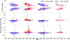 |
Fig. 1. Top panel: scatter plot of axial dipole moments of all active regions of cycles 21−24. The areas of the circles are proportional to the axial dipole moments of the active regions, and red and blue colors represent positive and negative axial dipole moments, respectively. Middle panel: rotational sums of negative and positive axial dipole moments for northern hemisphere. Bottom panel: rotational sums of negative and positive axial dipole moments for southern hemisphere. Vertical lines are axial dipole moment-weighted average emergence times of wings. Solid line is for the normal sign, dashed line for the opposite sign. |
The butterfly diagram of axial dipole moments is very similar to the more traditional butterfly diagram of sunspots. However, the wings are clearer and easier to separate than in a sunspot butterfly diagram. The unusually long activity minimum between cycles 23 and 24 is visible, as well as the weakness of cycle 24 compared to the rest of the cycles.
Figure 1 shows that, while the axial dipole moments of most active regions have the normal sign, active regions with axial dipole moments of opposite sign continuously appear. There is no strong preference for active regions with opposite dipole moments to emerge at some specific phase of the solar cycle. In the northern hemisphere for example, there are a few large positive (opposite-sign) peaks in 1979 and 1982. These few rotations form a large fraction of the total positive axial dipole moment of the respective wing, despite only being caused by a few active regions, as can also be seen in the top panel of Fig. 1. The corresponding peaks of opposite moment are, in fact, almost as high as the highest peak of normal (negative) sign of the same wing. The peak in 1979 is caused by an active region at the equator (AR 298 in Carrington rotation 1686, and AR 368 in Carrington rotation 1687). The positive polarity part is in the northern hemisphere, and the negative polarity part directly below it, partly in the southern hemisphere. Tilt orientation of this region is about 90°, relative to the equator. This unusual configuration causes the active region to have a large positive axial dipole moment. The peaks in 1982 are caused by two different active regions (AR 3673 in Carrington rotation 1725, and AR 4022 in Carrington rotation 1729). The first one is fairly large and violates Joy’s law. The leading positive polarity flux is at a higher latitude than the trailing negative polarity flux. The second one is similar to the one seen in 1979. The positive polarity part is again directly north of the negative polarity part, but in this case, the active region resides completely in the northern hemisphere, albeit at a low latitude. For a visual reference of these regions, they can be found in Solar-Geophysical Data No. 423, 424, 458, and 462 using the active region numbers given above (Coffey 1979a,b, 1982, 1983). Opposite-sign peaks are also found in the southern wing of cycle 22, and in all other wings as well, but their absolute and relative heights are smaller.
The axial dipole moments of normal sign tend to emerge, on average, earlier in the northern hemisphere than in the southern hemisphere. This can be seen from the average emergence times (solid vertical lines in the two lower panels of Fig. 1). This rule is valid for all four studied cycles. The average emergence time of opposite-sign axial dipole moment does not show a similar systematic hemispheric difference, but the rule is still true for all cycles, with the exception of cycle 22. The average emergence time of opposite-sign moment is later than the average emergence time of normal sign for all the six wings of cycles 21−23. In cycle 24, the axial dipole moment of normal sign emerges slightly later than the opposite-sign moment. This may be due to the still unfinished development of cycle 24. However, the current activity in the late declining phase of cycle 24 is so weak that this exceptional ordering may well remain valid, which would indicate a different, relatively more important role of the opposite-sign axial dipole moments for cycle 24. It should also be noted that the average emergence times in the north and south are closest to each other during cycle 24, both for normal-sign and opposite-sign moments. This is quite surprising since the rates of emergence have their maxima at quite different times in the two hemispheres, as seen in Fig. 1. Even sunspot maxima are known to be widely separate in the north (in 2012) and south (in 2014) for cycle 24.
It should be noted that very strong active regions that survive for multiple rotations may be included in this analysis multiple times, since active regions are identified separately from synoptic maps of all rotations. This means that the axial dipole moment of a very large active region may be included in the rotational sum of more than one rotation.
4. Axial dipole moments
Table 1 shows the number (N) of positive and negative axial dipole moments and their total moments (M), as well as the ratio (R) of the number of opposite sign-moments and all moments, and the (absolute) ratio (D) of opposite-sign moment, and the total absolute moment for each wing. It should be noted that the number and total moment of positive and negative axial dipole moments are given separately for Hale-ordered and anti-Hale active regions. The rows titled “Positive” or “Negative” include all positive or negative moments, respectively, the rows titled “Positive Hale” or “Positive anti-Hale” include all positive moments with Hale or anti-Hale polarities, respectively, and the rows titled “Negative Hale” or “Negative anti-Hale” include all negative moments with Hale or anti-Hale polarities, respectively. The “Opposite/total” ratio gives the ratio of number or total moment of opposite-polarity regions (unbolded in Table 1) to all regions. The total number of active regions varies significantly, from 690 in the southern wing of cycle 23 to 352 in the southern wing of cycle 24, but the number of opposite-sign moments is consistently about 30% of all moments in all wings.
Number of active regions (N) with positive and negative axial dipole moments, ratio of number of active regions (R) with opposite-sign axial dipole moments and total number of active regions, total positive and negative axial dipole moment (M, in Gauss), and the ratio of axial dipole moment of opposite sign and the total absolute axial dipole moment (D).
In the wings of cycles 21−23, there is typically about 4−5 G of normal-sign axial dipole moment, and 1−2 G of opposite-sign axial dipole moment. The southern wing of cycle 22 shows by far the largest amount of normal axial dipole moment, but it does not show an unusually large number of opposite moments. The large axial dipole moment at this time is caused by a few large active regions with normal-sign moments, which can be seen in Fig. 1 as the highest in the center of the activity belt in 1991. The axial dipole moment of cycle 24 is less than half of the earlier cycles. The number of active regions is also lower, but the relative change is not as large, indicating that the average axial dipole moment of an active region is smaller in cycle 24 than in earlier cycles. Interestingly, there are more active regions (both of normal sign and total) in the southern wing than in the northern wing during cycles 21−23, but during cycle 24, there are more active regions of both the normal and opposite sign in the northern wing.
The fraction of opposite-sign axial dipole moments varies between the wings from 0.16 to 0.29. The northern wing of cycle 21 has the largest fraction, while the northern wing of cycle 23 has the smallest. The large fraction of cycle 21 is caused by a few large opposite-sign regions in the northern wing (see Fig. 1). The four rotations with the largest opposite-sign moments in 1979 and 1982 contain almost 0.2 G each, which together account for the majority of the difference between the northern wings of cycles 21 and 23. The ratio of opposite-sign moment and total absolute moment varies more, and is smaller than the ratio of the number of opposite-sign moments and the total number of moments in all wings. This indicates that opposite-sign moments are on average smaller than normal-sign moments.
The number of active regions with anti-Hale polarity is relatively low. About 6% of all active regions are anti-Hale, and about 10% of active regions with opposite-sign axial dipole moments are anti-Hale. These numbers are fairly close to the results of McClintock et al. (2014), who found 8.4% of all sunspot groups to have anti-Hale polarity (for review, see Pevtsov et al. 2014). The vast majority of opposite-sign axial moments are caused by violations of (only) Joy’s law, from a Hale-ordered active region where the trailing polarity part is at a lower latitude than the leading polarity part. The number of anti-Hale regions with negative and positive axial dipole moments is fairly similar in all wings. There are in total 267 anti-Hale active regions, and, out of those, 126 have opposite-sign axial dipole moments. This implies that anti-Hale active regions do not typically follow Joy’s law. The average absolute sizes of opposite-sign moments with Hale and anti-Hale polarities are 0.006 G and 0.014 G, respectively. This indicates that active regions that violate Hale’s law have, on average, larger axial dipole moments than active regions that violate Joy’s law, and that the two populations may have different characteristics. However, the number of anti-Hale active regions is too low to analyze their distribution in detail. Therefore, we do not divide the opposite-sign moments into two groups, those resulting from a violation of Hale’s law and those from Joy’s law.
5. Latitude distributions
Figure 2 shows the latitudinal distributions of positive and negative axial dipole moments for each wing of the four cycles. In the two upper rows, the negative and positive moments of each wing have been summed separately in five degree bins. In the bottom panels each bin of negative moment has been divided by the total negative moment of the respective wing and each bin of positive moment by the total positive moment of the wing. These normalized distributions are not affected by the varying total moment of the wings, and the height of the bars give the fraction of the total negative or positive moment of a wing contained in each bin. The vertical axis of cycles 21 and 23 have been reversed so that the moments of normal sign are always in the upward direction.
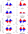 |
Fig. 2. Latitudinal distribution of positive (red) and negative (blue) axial dipole moment for wings of cycles 21−24. Top four panels: unnormalized sums. Bottom four panels: negative and positive bins of each wing have been normalized separately by the respective total sums, so that the sum of the heights of the bars is one. Bin width is five degrees. |
In cycles 21−23, the highest peak of the normal sign is in the southern hemisphere in both the unnormalized and normalized distributions. This suggests that the emergence of flux starts earlier in the northern hemisphere, which produces relatively more axial dipole moment at higher latitudes and over a larger latitude range in the northern hemisphere than in the south. In cycle 24, the unnormalized peak is slightly higher in the southern hemisphere, but the normalized peak is somewhat higher in the northern hemisphere. In cycles 21 and 24, the bins with highest values are in both wings at 10 ° −15°, and in cycle 22 at 15 ° −20°. In cycle 23, the maximum in the north is at a higher latitude, at 20 ° −25°, while the maximum in the south is at 15 ° −20°. Thus, the maximum contribution to dipole moments comes from active regions at 10 ° −20° latitude.
The distributions of opposite-sign axial dipole moments vary significantly from wing to wing, and are different from the distributions of normal-sign moments. Both wings of cycle 23 have distributions that are rather flat over a wide latitude range. The northern wing of cycle 22 is also fairly flat, apart from the peak at low latitudes. There is no systematic difference in the latitude distributions between hemispheres, contrary to the normal-sign moments, nor any systematic similarity or difference between the four cycles. It seems that the emergence of small opposite-sign active regions is fairly random in the activity belts.
6. Axial dipole moment histograms
Figure 3 shows histograms of axial dipole moments separately for the northern and southern wings of cycles 21−24. The histograms have been normalized by the total number of moments in each wing, so that the heights of the bars give the relative number of moments in each bin, which also serves as an estimate of the probability of a moment falling within a bin. As for Fig. 2, the axial dipole moments (horizontal axis) of cycles 21 and 23 have been reversed, so that the normal-sign moments are always on the right. The bin size is 0.01 G.
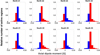 |
Fig. 3. Histograms of axial dipole moments of active regions for northern and southern wings of cycles 21−24. Bin size is 0.01 G. Red bars are for positive moments, blue bars are for negative moments. |
The normal-sign moment histograms are markedly similar close to zero in cycles 21−23. The first bin of normal-sign moments varies between 0.46 and 0.49, and the second bin between 0.9 and 0.11. Cycle 24 has a larger fraction of small moments (and a larger hemispheric asymmetry), the first bin having a value of 0.58 in the north, and 0.53 in the south. For larger axial dipole moments, the number of active regions is too small to draw significant conclusions of possible differences between the distributions.
For opposite-sign moments, the first bin is between 0.23 and 0.27 for all wings except the southern wing of cycle 22, which has a slightly lower value of 0.20. This means that the first bin of opposite-sign moments typically has roughly half as many active regions as the first bin of normal-sign moments. However, there are few large opposite-sign moments, and the distribution drops more steeply with the absolute value of axial dipole moment compared to the normal-sign moments, reflecting the smaller average strength of opposite-sign moments seen in Table 1. Notably, cycle 24 does not differ from the rest of the cycles in this sense.
Figure 4 shows separate histograms for all normal-sign and for all opposite-sign moments of cycles 21−24. As in Fig. 3, the histograms have been normalized by the respective total numbers. The distributions clearly show the larger relative number of small moments of opposite-sign, which is also seen in Table 1 and in Fig. 3. The distributions of normal-sign and opposite-sign moments are both centered at zero, but the distribution of opposite-sign moments is narrower with a higher peak.
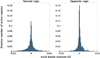 |
Fig. 4. Histograms of axial dipole moments of active regions of normal sign (left) and opposite sign (right). All active regions of cycles 21−24 are included. Bin size is 0.001 G. |
7. Axial dipole moments vs. magnetic fluxes
Figure 5 shows the axial dipole moments of active regions as a function of the unsigned flux of the active regions. All eight wings of cycles 21−24 were plotted separately. The vertical axes of cycles 21 and 23 were reversed so that moments of the normal sign are always in the upper part of the plot. Active regions of all wings appear almost exclusively inside a cone opening from zero, implying that a sufficient amount of flux is required for a certain axial dipole moment. However, a large total flux does not guarantee a large axial dipole moment. Many of even the strongest active regions have axial dipole moments close to zero, due to a very small tilt angle. On the other hand, sometimes an active region with only a moderate total flux can have a substantial axial dipole moment. Most notably in the northern wing of cycle 21, we can see a few opposite-sign active regions outside (below) the main cone. These are the large opposite-sign moments seen in Fig. 1. They have, in fact, some of the largest axial moments of the cycle, even though their total flux is not very strong.
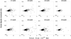 |
Fig. 5. Axial dipole moments of active regions as a function of their total unsigned flux, separately for the northern and southern wings of cycles 21−24. |
At low total fluxes, there is a large number of small moments in every wing, and they are distributed fairly randomly around zero at the approximate 2 : 1 ratio discussed above. For larger total fluxes, the moments are more clearly concentrated to the normal-sign side. At very large total fluxes, there is more scatter and also clear differences between cycles. In cycle 22, there are many active regions with very large total fluxes and axial dipole moments. They are responsible for the large total axial dipole moment of the southern wing seen in Table 1. In cycle 24, on the other hand, almost all active regions have fairly low total fluxes. Only two active regions in the southern hemisphere have a total flux above 2 × 10²² Mx, and even they have relatively small axial dipole moments. Since almost all data points are situated within a cone, especially those below about 0.5 × 10²² Mx, there appears to be an upper limit on the axial dipole moment for a certain flux. This may be due to a limited range of tilt values of the decaying active regions. Figure 5 also suggests that there may be a separate population of large total flux, which behaves differently to the more compact low total flux population.
8. Discussion
Previous studies of the effect of active region orientation on solar polar fields have typically treated the Hale polarity law and Joy’s tilt law separately. Here we have studied the axial dipole moment of active regions, which combines Hale’s and Joy’s laws and provides an effective measure of the impact of active regions on solar large-scale dipole (polar) fields. We find that even anti-Hale active regions may contribute to the normal axial dipole moment of the solar large-scale dipole, if these regions also deviate from Joy’s law. Similarly, active regions whose tilt orientation deviates from Joy’s law may reduce the solar dipole if they follow the Hale polarity rule.
We studied the axial dipole moments of active regions observed in the photospheric magnetic field during cycles 21−24. We find that there is a significant number of active regions whose axial dipole moments have a sign opposite to the normal sign expected from Joy’s and Hale’s laws. Some 16 − 29% of the total emerging axial dipole moment, and 27 − 32% of the total number of emerging active regions in each butterfly wing, have an oppositely signed axial dipole moment. Most of the opposite-sign moment comes from small opposite-sign active regions which have Hale polarity but do not follow Joy’s law. As seen in Fig. 1, they can emerge in any part of the activity belts in both hemispheres, regardless of latitude or time. About 6% of all active regions have anti-Hale polarity, which is close to previous estimates of the number of anti-Hale sunspot groups.
We find that the relative number of small opposite-sign moments is roughly similar in all wings of cycles 21−24. Large opposite-sign moments are rare, but they can contribute very significantly to the total axial dipole moment of a cycle. This is particularly clear in case of the northern hemisphere of cycle 21 and the southern hemisphere of cycle 22. The opposite-sign moments are, on average, smaller than normal-sign moments. As seen in Fig. 4, the distribution of opposite-sign moments is narrower and has a higher peak around zero than the distribution of normal-sign moments. This implies that the axial dipole moments of opposite sign tend to be smaller.
We find a hemispherical asymmetry in the occurrence of axial dipole moments with the expected (normal) sign. The northern hemisphere activates earlier in cycles 21−23, and a relatively larger amount of axial dipole moment emerges at higher latitudes than in the southern hemisphere. Opposite-sign moments do not show this hemispherical asymmetry, but emerge, on average, later than normal-sign moments in all wings of cycles 21−23.
Although cycle 24 is not quite finished, it seems quite likely that cycle 24 significantly differs from cycles 21−23. Cycle 24 contains the lowest number of active regions, and has the smallest amount of axial dipole moment. It is the only cycle where the northern wing contains more active regions than the southern wing. However, the northern surplus is only in small moments, and the southern wing contains more normal-sign axial dipole moment than the northern wing. The relative number of small normal-sign moments is higher in cycle 24 than in cycles 21−23, especially in the northern hemisphere. There are very few large moments, and the average moment is smaller than in previous cycles. Cycle 24 is also the only cycle where the axial dipole moment-weighted emergence time of active regions is slightly earlier for opposite-sign moments than for normal-sign moments.
Acknowledgments
We acknowledge the financial support by the Academy of Finland to the ReSoLVE Centre of Excellence (project no. 307411). The National Solar Observatory (NSO) is operated by the Association of Universities for Research in Astronomy, AURA Inc under cooperative agreement with the National Science Foundation (NSF). The data used in this work were produced in the framework of the NSO synoptic program. HMI data are courtesy of the Joint Science Operations Center (JSOC) Science Data Processing team at Stanford University. This work was partially supported by the International Space Science Institute (Bern, Switzerland) via International Team 420 on Reconstructing Solar and Heliospheric Magnetic Field Evolution over the Past Century.
References
- Baranyi, T. 2015, MNRAS, 447, 1857 [Google Scholar]
- Baumann, I., Schmitt, D., Schüssler, M., & Solanki, S. K. 2004, A&A, 426, 1075 [NASA ADS] [CrossRef] [EDP Sciences] [Google Scholar]
- Coffey, H. E. 1979a, Solar-geophysical Data Number 423, part 1. Prompt reports: Data for October 1979, September 1979, Tech. rep., https://www.ngdc.noaa.gov/stp/space-weather/online-publications/stp_sgd/1979/sgd7911p.pdf [Google Scholar]
- Coffey, H. E. 1979b, Solar-geophysical Data Number 424, part 1 (prompt reports). Data for November 1979, October 1979, Tech. rep., https://www.ngdc.noaa.gov/stp/space-weather/online-publications/stp_sgd/1979/sgd7912p.pdf [Google Scholar]
- Coffey, H. E. 1982, Solar-geophysical Data Number 458, October 1982. Part 1: (Prompt reports). Data for September 1982, August 1982 and late data, Tech. rep., https://www.ngdc.noaa.gov/stp/space-weather/online-publications/stp_sgd/1982/sgd8210p.pdf [Google Scholar]
- Coffey, H. E. 1983, Solar-geophysical Data Number 462, part 1. Prompt reports, data for January 1983 – December 1982 and late data, Tech. rep., https://www.ngdc.noaa.gov/stp/space-weather/online-publications/stp_sgd/1983/sgd8302p.pdf [Google Scholar]
- Hale, G. E., & Nicholson, S. B. 1925, ApJ, 62, 270 [NASA ADS] [CrossRef] [Google Scholar]
- Hale, G. E., Ellerman, F., Nicholson, S. B., & Joy, A. H. 1919, ApJ, 49, 153 [NASA ADS] [CrossRef] [Google Scholar]
- Jiang, J., Cameron, R., Schmitt, D., & Schüssler, M. 2010, ApJ, 709, 301 [NASA ADS] [CrossRef] [Google Scholar]
- Jiang, J., Cameron, R. H., Schmitt, D., & Schüssler, M. 2011, A&A, 528, A82 [NASA ADS] [CrossRef] [EDP Sciences] [Google Scholar]
- Jiang, J., Cameron, R. H., & Schüssler, M. 2014, ApJ, 791, 5 [Google Scholar]
- Jones, H. P., Duvall, Jr., T. L., Harvey, J. W., et al. 1992, Sol. Phys., 139, 211 [NASA ADS] [CrossRef] [Google Scholar]
- Keller, C. U., Harvey, J. W., & Giampapa, M. S. 2003, in Innovative Telescopes and Instrumentation for Solar Astrophysics, eds. S. L. Keil, & S. V. Avakyan, Proc. SPIE, 4853, 194 [NASA ADS] [CrossRef] [Google Scholar]
- Li, J., & Ulrich, R. K. 2012, ApJ, 758, 115 [NASA ADS] [CrossRef] [Google Scholar]
- Livingston, W. C., Harvey, J., Slaughter, C., & Trumbo, D. 1976, Appl. Opt., 15, 40 [NASA ADS] [CrossRef] [Google Scholar]
- McClintock, B. H., Norton, A. A., & Li, J. 2014, ApJ, 797, 130 [NASA ADS] [CrossRef] [Google Scholar]
- Pevtsov, A. A., Berger, M. A., Nindos, A., Norton, A. A., & van Driel-Gesztelyi, L. 2014, Space Sci. Rev., 186, 285 [Google Scholar]
- Pevtsov, A. A., Virtanen, I., Mursula, K., Tlatov, A., & Bertello, L. 2016, A&A, 585, A40 [NASA ADS] [CrossRef] [EDP Sciences] [Google Scholar]
- Pietarila, A., Bertello, L., Harvey, J. W., & Pevtsov, A. A. 2013, Sol. Phys., 282, 91 [NASA ADS] [CrossRef] [Google Scholar]
- Riley, P., Ben-Nun, M., Linker, J. A., et al. 2014, Sol. Phys., 289, 769 [Google Scholar]
- Virtanen, I., & Mursula, K. 2017, A&A, 604, A7 [NASA ADS] [CrossRef] [EDP Sciences] [Google Scholar]
- Virtanen, I. O. I., Virtanen, I. I., Pevtsov, A. A., Yeates, A., & Mursula, K. 2017, A&A, 604, A8 [NASA ADS] [CrossRef] [EDP Sciences] [Google Scholar]
- Virtanen, I. O. I., Virtanen, I. I., Pevtsov, A. A., & Mursula, K. 2018, A&A, 616, A134 [NASA ADS] [CrossRef] [EDP Sciences] [Google Scholar]
- Wang, Y.-M., & Sheeley, Jr., N. R. 1991, ApJ, 375, 761 [NASA ADS] [CrossRef] [Google Scholar]
- Whitbread, T., Yeates, A. R., Muñoz-Jaramillo, A., & Petrie, G. J. D. 2017, A&A, 607, A76 [NASA ADS] [CrossRef] [EDP Sciences] [Google Scholar]
- Yeates, A. R., Baker, D., & van Driel-Gesztelyi, L. 2015, Sol. Phys., 290, 319 [Google Scholar]
All Tables
Number of active regions (N) with positive and negative axial dipole moments, ratio of number of active regions (R) with opposite-sign axial dipole moments and total number of active regions, total positive and negative axial dipole moment (M, in Gauss), and the ratio of axial dipole moment of opposite sign and the total absolute axial dipole moment (D).
All Figures
|
Fig. 1. Top panel: scatter plot of axial dipole moments of all active regions of cycles 21−24. The areas of the circles are proportional to the axial dipole moments of the active regions, and red and blue colors represent positive and negative axial dipole moments, respectively. Middle panel: rotational sums of negative and positive axial dipole moments for northern hemisphere. Bottom panel: rotational sums of negative and positive axial dipole moments for southern hemisphere. Vertical lines are axial dipole moment-weighted average emergence times of wings. Solid line is for the normal sign, dashed line for the opposite sign. |
| In the text | |
|
Fig. 2. Latitudinal distribution of positive (red) and negative (blue) axial dipole moment for wings of cycles 21−24. Top four panels: unnormalized sums. Bottom four panels: negative and positive bins of each wing have been normalized separately by the respective total sums, so that the sum of the heights of the bars is one. Bin width is five degrees. |
| In the text | |
|
Fig. 3. Histograms of axial dipole moments of active regions for northern and southern wings of cycles 21−24. Bin size is 0.01 G. Red bars are for positive moments, blue bars are for negative moments. |
| In the text | |
|
Fig. 4. Histograms of axial dipole moments of active regions of normal sign (left) and opposite sign (right). All active regions of cycles 21−24 are included. Bin size is 0.001 G. |
| In the text | |
|
Fig. 5. Axial dipole moments of active regions as a function of their total unsigned flux, separately for the northern and southern wings of cycles 21−24. |
| In the text | |
Current usage metrics show cumulative count of Article Views (full-text article views including HTML views, PDF and ePub downloads, according to the available data) and Abstracts Views on Vision4Press platform.
Data correspond to usage on the plateform after 2015. The current usage metrics is available 48-96 hours after online publication and is updated daily on week days.
Initial download of the metrics may take a while.