| Issue |
A&A
Volume 631, November 2019
|
|
|---|---|---|
| Article Number | A118 | |
| Number of page(s) | 16 | |
| Section | Catalogs and data | |
| DOI | https://doi.org/10.1051/0004-6361/201936485 | |
| Published online | 05 November 2019 | |
A stellar census in globular clusters with MUSE: A spectral catalogue of emission-line sources⋆
1
Institut für Astrophysik, Georg-August-Universität Göttingen, Friedrich-Hund-Platz 1, 37077 Göttingen, Germany
e-mail: This email address is being protected from spambots. You need JavaScript enabled to view it.
2
Astrophysics Research Institute, Liverpool John Moores University, 146 Brownlow Hill, Liverpool L3 5RF, UK
3
Leibniz-Institut für Astrophysik Potsdam (AIP), An der Sternwarte 16, 14482 Potsdam, Germany
4
Institut für Physik und Astronomie, Universität Potsdam, Karl-Liebknecht-Str. 24/25, 14476 Golm, Germany
Received:
9
August
2019
Accepted:
10
September
2019
Abstract
Aims. Globular clusters produce many exotic stars due to a much higher frequency of dynamical interactions in their dense stellar environments. Some of these objects were observed together with several hundred thousand other stars in our MUSE survey of 26 Galactic globular clusters. Assuming that at least a few exotic stars have exotic spectra (i.e. spectra that contain emission lines), we can use this large spectroscopic data set of over a million stellar spectra as a blind survey to detect stellar exotica in globular clusters.
Methods. To detect emission lines in each spectrum, we modelled the expected shape of an emission line as a Gaussian curve. This template was used for matched filtering on the differences between each observed 1D spectrum and its fitted spectral model. The spectra with the most significant detections of Hα emission are checked visually and cross-matched with published catalogues.
Results. We find 156 stars with Hα emission, including several known cataclysmic variables (CV) and two new CVs, pulsating variable stars, eclipsing binary stars, the optical counterpart of a known black hole, several probable sub-subgiants and red stragglers, and 21 background emission-line galaxies. We find possible optical counterparts to 39 X-ray sources, as we detected Hα emission in several spectra of stars that are close to known positions of Chandra X-ray sources. This spectral catalogue can be used to supplement existing or future X-ray or radio observations with spectra of potential optical counterparts to classify the sources.
Key words: globular clusters: general / stars: emission-line, Be / novae, cataclysmic variables / catalogs / techniques: imaging spectroscopy
Table A.2 and spectra (FITS) are available at the CDS via anonymous ftp to cdsarc.u-strasbg.fr (130.79.128.5) or via http://cdsarc.u-strasbg.fr/viz-bin/cat/J/A+A/631/A118
© ESO 2019
1. Introduction
In the dense stellar environments of globular clusters (GCs), the frequent interactions between stars produce a wealth of stellar exotica. This includes interacting binary systems and end states of stellar evolution, such as cataclysmic variables (CVs, Ivanova et al. 2006), pulsars (Ransom 2007), and planetary nebulae (PNe; Jacoby et al. 2017). Emission lines are expected to appear in the optical spectra in at least some of these stellar types; those stars are then classified as emission-line stars. Because of the old age of globular clusters and their stars, some types of emission-line stars still present in the Milky Way disc do not exist (anymore) in globular clusters, for example Wolf-Rayet stars or Be stars.
In recent years, several stellar-mass black hole (BH) candidates have been found in binary systems in globular clusters (Strader et al. 2012; Giesers et al. 2018). Photometric observations suggest that some of these systems could be Hα emitters. While stellar-mass BHs were long thought to be ejected from GCs during cluster evolution, the discoveries of stellar-mass BH candidates in multiple clusters indicate a large population of these black holes inside evolved GCs (Strader et al. 2012; Askar et al. 2018; Kremer et al. 2018).
Cataclysmic variables are binary systems consisting of a hot, compact white dwarf and a dwarf star in a close orbit. The white dwarf accretes material from its companion star that accumulates in an accretion disc. In the dense stellar environments of globular clusters, CVs and progenitor systems are influenced by dynamical interactions, with up to 50% forming via a binary encounter (Ivanova et al. 2006, but also see Belloni et al. 2019). The number of predicted CVs per cluster is of the order of 200, but the number of observed CV candidates or confirmed CVs in the literature is much lower (Knigge 2012). CV candidates can be found with photometric observations, for example by looking for dwarf nova outbursts, for stars with UV excess (e.g. Rivera Sandoval et al. 2018), for outliers in the colour-magnitude diagram (CMD) of a GC (e.g. Campos et al. 2018), or by using Hα surveys (Knigge 2012). Alternatives for detecting CVs are far-ultraviolet spectroscopy which has also been useful for detecting CVs in globular clusters (Knigge et al. 2003), and X-ray observations. Follow-up optical spectroscopy to confirm CVs in GCs is difficult because of the crowded fields and the intrinsically low brightness of CVs.
When a nova occurs in a CV, it can leave behind a visible emission nebula as a remnant such as the one in NGC 6656 (Göttgens et al. 2019). Nova remnants are not the only type of nebula in GCs; another type are planetary nebulae of which four are known in the Galactic GC system. Even this low number of PNe in GCs is too high because the low masses of AGB stars should prohibit the formation of PNe (Jacoby et al. 1997). This lead to the prediction that PNe in GCs are formed by a different mechanism, possibly by binary interaction (Jacoby et al. 1997, 2017).
Many stellar exotica in GCs have been found using X-ray observations. However, it is less clear which optical counterpart belongs to an X-ray source when only broad-band photometry is available. In this case, a counterpart is identified if it is an outlier in the optical CMD with respect to all other cluster stars, that is if its separation from the main sequence or the red-giant branch (RGB) is too large, or if its colour is too blue (e.g. Bassa et al. 2004; Webb et al. 2004). Similarly, the presence of optical emission lines in a spectrum of a star close to an X-ray source could also indicate it is a counterpart.
Previous optical surveys for typical classes of emission-line objects used photometric observations and the on/off-band technique, variability, or anomalous colours to detect candidate objects: Jacoby et al. (1997) conducted the most successful PNe survey for GCs, Knigge (2012) lists several CV surveys. Spectroscopic follow-up observations are then used to confirm the classification and to derive more properties of the source.
The data used in this paper were obtained with the Multi Unit Spectroscopic Explorer (MUSE, Bacon et al. 2010), a panoramic integral-field spectrograph at the Very Large Telescope, as part of a survey of Galactic globular clusters. With the MUSE data already obtained, emission-line objects can be found without the need of additional observations because both spatial and spectral information is present. While Roth et al. (2018) demonstrated the efficiency of MUSE at detecting emission-line objects including Wolf-Rayet stars, supernova remnants, H II regions, and PNe in the galaxy NGC 300, we can for the first time conduct a blind survey for emission-line stars in Galactic globular clusters.
2. Data
2.1. Observations and reduction
This work makes use of all data taken with MUSE for our survey of 26 Galactic globular clusters between September 2014 and March 2019 (PI: S. Dreizler, S. Kamann)1. MUSE has a large field of view (1′×1′) combined with a spatial sampling of 0.2″ and an intermediate resolution R between 1800 and 3500 in the spectral range from 4750 to 9350 Å. The observations and the analysis steps are described in detail by Kamann et al. (2018) and are summarised here. In contrast to Kamann et al. (2018), this work also includes data from observations made after October 2016. Table 1 gives an overview of the observation statistics for each cluster.
Overview of globular cluster data used in this paper.
Each observation was reduced with the standard MUSE pipeline (Weilbacher et al. 2012, 2014) which calibrates the images from the 24 MUSE spectrographs, including cosmic ray rejection, and transforms them into a datacube. In the next step, single stellar spectra are extracted with a point-spread-function (PSF) from this datacube. The extractions use the PSF-fitting developed in Kamann et al. (2013) to measure the PSF parameters and determine stellar positions in the datacube as a function of wavelength. We mostly used stellar positions from the Hubble Space Telescope (HST) ACS survey of Galactic globular clusters (hereafter ACS catalogue, Sarajedini et al. 2007; Anderson et al. 2008) as an input for the extraction, see Table 2 in Kamann et al. (2018) for details. The extracted spectra were then analysed with respect to the Göttingen spectral library (Husser et al. 2013), a grid of synthetic spectral models suitable for most stars in globular clusters. A chi-square fit on the full spectrum minimises the difference between the observed spectrum and a model spectrum by interpolating between grid spectra to determine the stellar parameters effective temperature, metallicity, and the radial velocity (Husser et al. 2016).
In addition to the spectra obtained from single observations, we also used these to create a high-signal-to-noise spectrum for each star. We shifted all spectra of each star to the Sun’s restframe and added the flux weighted by the signal-to-noise (S/N) ratio of the spectrum. These combined spectra were then analysed in a similar way to the one described above.
2.2. Residuals from spectral fitting
The residuals from the spectral fitting are defined as the difference between model and observation. We can use these residuals to detect emission-line stars because the spectral library does not contain spectra with emission lines; in other words, if an emission line is present in the observed spectrum, it will also be visible in the residuals.
The residuals can contain random noise, additional absorption from the interstellar medium (Wendt et al. 2017), systematic errors of the model spectra (e.g. absorption lines that only exist in the models, see Fig. 1, or vice versa), instrumental systematics, and true emission lines. If the fit does not find the global minimum of the chi-square space, the residuals will contain a large amount of stellar light. In this case, the parameters determined by the fit do not necessarily describe the star, and the residuals can cause false positive detections of emission lines.
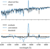 |
Fig. 1. Illustration of emission-line detection with matched filtering. Top: observed flux of V190 in NGC 6266 with Hα emission and the fitted spectral model. Bottom: Hα emission line is still present in the residuals, as well as an absorption line at 6700 Å which is only found in the models. The convolution with a Gaussian increases the emission line above the threshold calculated from the mean absolute deviation of the residuals. |
It is also possible that the spectral model grid does not contain a suitable model for the observed spectrum. This occurs for horizontal branch stars and some M stars. Spectra of M stars contain strong molecular bands which have a great influence on the overall spectral appearance. A slight mismatch in the fit of an M star spectrum has a large impact on the residuals. If a spectrum of an M star contains emission lines, the effect of the emission lines on the residuals could be smaller than the effects of spectrum mismatch. In these cases, the method based on matched filtering to detect emission lines described in Sect. 3.1 was not reliable and the detection failed. However, the method based on the residuals without convolution (Sect. 3.2) still worked in these cases.
3. Emission line detection
As shown in Table 1, we extracted millions of stellar spectra from our observations. The large number of observed spectra makes it impossible to visually check each of them.
We used two approaches to detect emission lines in the residuals from the spectral fit. The first approach based on matched filtering is widely applied to similar problems, for example in gravitational-wave detection (Abbott et al. 2016) and to detect emission-line galaxies in MUSE datacubes (Herenz & Wisotzki 2017). The second method uses only the residuals and a running estimate of the noise. This method is used as a backup whenever matched filtering fails to detect a signal, because it is much simpler and more robust but also produces more false detections. Both approaches assign a significance to each detection which is then used to select the most promising candidates for visual inspection.
We stress that we did not use existing catalogues of emission-line stars as a prior to find those in our data. Since the aim of this work is to find new and unexpected sources, we used external catalogues only after our methods identify a possible spectrum with emission lines.
3.1. Matched filtering with mean absolute deviation
Because of the large dataset, we needed to choose an approach that is fast and can extract potentially weak signals. One algorithm with these properties is called matched filtering (see Vio & Andreani 2016, and references therein) that requires prior knowledge about the expected signal. We assumed that each emission line can be described by a Gaussian curve with a standard deviation (width) of 5 Å. This width is determined from simulations in Sect. 3.3. Instead of applying matched filtering directly on the observed spectral flux (top panel in Fig. 1), we used it on the residuals that result from spectral fitting (see bottom panel of Fig. 1). Mathematically, matched filtering computes the convolution C(λ) of the filter (the expected line profile) and the residual flux. As shown in the bottom panel in Fig. 1 (dashed line), the convolution is high at a certain wavelength when the expected flux shape matches the measured flux. On the other hand, noise – which is typically only a few pixels wide – is smoothed out, that means the convolution gives a much lower value as it would for real emission. Compared to the convolution of noise or continuum flux with a Gaussian, emission flux appears in the convolution as a peak centred at the emission line. We detect an emission signal at wavelength λe if the convolution at that point is larger than some threshold function t(λ) at the same point. The threshold function is constructed as the median absolute deviation calculated separately for wavelength bins of the residual flux (dotted line in the bottom panel of Fig. 1). By construction, the ratio Ds = C(λe)/t(λe) is higher for more prominent emission signals. We call this ratio detection significance and use it to select promising candidates for visual inspection by requiring that a detection lies above a minimum value of Ds. The detection efficiency depends on this choice and it is analysed with simulated emission lines in Sect. 3.3.
3.2. Plain residuals and running noise estimate
This section presents a more robust method of detecting emission lines that relies on fewer assumptions. Similar to the method based on matched filtering, it relies on the residuals from the spectral fit. The residual flux ri = r(λi) at each wavelength point λi is compared to the residual noise si at the adjacent wavelengths. We locally estimated the noise from the difference of the ninetieth and tenth percentile of the residual flux in a 100 Å window centred at λi. Since the spectral model does not describe the observed flux perfectly, the residuals contain noise and systematic effects (see Sect. 2.2). We accounted for these outliers in the residual flux by using percentiles instead of extrema or measures that are sensitive to outliers. At each wavelength, the ratio of residual flux to the noise estimate Ds = ri/si represents the significance of an emission-line detection. For comparison, if the noise was normally distributed with a variance σ2, a ratio of Ds = 1 corresponds to an observation with a significance of ≈1.3σ.
Simulations showed that this method works well for narrow emission lines but not for broad ones. This is because a broad emission line increases the residuals over a broader spectral range, and thus the percentiles used to estimate the noise increase as well. Since this increases si but not the amplitude ri, the detection significance Ds decreases accordingly.
3.3. Detection efficiency
We estimated the fraction of emission signals recovered with the method based on matched filtering described in Sect. 3.1 with simulated emission lines. The detection significance of an emission-line candidate depends on the amplitude and width of the emission peak in the residual flux, and on the noise of the spectrum and the width of the Gaussian filter. We constructed emission lines by sampling a Gaussian curve with a standard deviation σ that we vary between 3 and 60 Å, its amplitude is set to one. We drew noise from a normal distribution with a width of (S/N)−1 and add it to the signal. For each simulated emission line, we applied the detection method (Sect. 3.1) and calculated the detection significance for filter widths of 6, 25, 60, and 120 Å. We note that this leads to an estimate of how effective the detection methods is with respect to the amplitude of an emission line and not the total line flux.
The main results of this analysis were: we can find broad synthetic emission lines of several tens of Ångström even with a narrow filter width of 6 Å while the reverse is not true. As Fig. 2 shows, we recovered about 50% of broad emission lines (≈40 Å) with a filter width of 6 Å for a S/N of 2 if we only take detections with Ds > 7.5 into account. This fraction increased with increasing S/N and with decreasing emission-line width (except for very narrow widths < 5 Å below the filter width). We concluded from these simulated emission lines that for our data the choice of a 6 Å filter is reasonable, and Ds > 7.5 is a good lower limit for a detection to be inspected further. The filter width is four to five times the FWHM of the line-spread-function (LSF) of MUSE which varies between 2.5 and 3 Å depending on wavelength (Bacon et al. 2017). In principle, one could choose the threshold Ds much lower than this for the price of many more detections to inspect, which will contain a much higher frequency of false positives. The choice of Ds > 7.5 is also justified by the low empirical true positive rate of ≲5% below this limit (see Sect. 4.1 and Fig. 4).
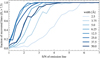 |
Fig. 2. Fraction of simulated emission lines that are recovered with a filter width of 6 Å depending on the simulated line width. Only detections above a detection significance Ds > 7.5 are taken into account. |
3.4. Limiting flux
The results of the simulations above were used to calculate the minimum amplitude of an emission line that can be detected. Since we selected detections with a significance above 7.5, emission lines in spectra with too high noise will not be found. From the simulations, we first estimated the minimum signal-to-noise ratio S/Nmin for that 80% of simulated emission lines are found. This S/Nmin depends on the width of the simulated emission line. Here, we chose a width of 40 Å, corresponding to CVs. The minimum signal that we could detect is estimated by measuring the noise σ in the residuals of all spectra from 6000 Å to 7000 Å. In practice, the noise depends on the brightness of the target star, observing conditions, stellar crowding, etc. We measured this effective noise in the residuals obtained from the spectral fitting. The minimum detectable signal in each spectrum is Fmin = S/Nmin ⋅ σ. Table 2 lists Fmin of a broad emission line for different representative points in the stellar population of each cluster we observed, and Fig. 3 shows the limiting flux as a function of stellar brightness in three clusters. Since we used a S/Nmin for which 80% of simulated emission lines are found, Table 2 gives the limiting flux for which 80% of all spectra with an emission line are found. Because we used a narrow filter width of 5 Å to detect emission lines, the limits given for a broad emission line can be treated as a conservative estimate of the limiting flux of narrow emission lines. The limiting fluxes for narrow emission lines generally fall inside the uncertainties given in Table 2, this means that this table is also valid for narrow lines. Depending on the brightness of the target star, we find that Fmin is generally between 10−17 and 10−16 erg s−1 cm−2 Å−1. To our knowledge, this is the first optical emission-line survey estimating the upper limit of fluxes for sources that remain undetected.
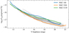 |
Fig. 3. Limiting flux for which 80% of sources will be detected as determined from simulated emission lines for different clusters as a function of brightness. Each grey curve represents a GC, the clusters NGC 104, NGC 3201, and NGC 5139 are highlighted. |
Limiting fluxes for all clusters, calculated using a broad emission line (40 Å) and also valid for narrow lines (see text).
4. The catalogue of emission-line sources
4.1. Results of visual inspection
We applied both detection methods to spectra extracted from MUSE observations of globular clusters (see Sect. 2.1) that have an S/N of at least five. Setting this threshold ensures that the spectral fit gives meaningful residuals. We wanted to inspect promising emission-line spectra visually. As this would have been very time consuming with thousands of candidate spectra, we checked candidate spectra which contain an emission line close to Hα (between 6540 and 6580 Å) if Ds > 7.5. With this set-up, we expect to find emission-line stars, typically Hα emitters, while galaxies would remain undetected. Section 4.7 describes how we find galaxies using all detected emission lines. In total, 1200 individual stars have at least one such spectrum, with a total of about 9000 spectra.
For each spectrum, we checked if the emission line could be valid according to a set of criteria. The potential emission line has to be at least two pixels wide (a pixel corresponds to 1.25 Å) and it must fulfil at least one of the following criteria:
-
The line candidate appears in roughly the same position with the same shape in multiple spectra of the same star, or
-
the spectrum shows emission lines in addition to Hα, or
-
the corresponding star is listed in the Catalogue of Variable Stars in Galactic Globular Clusters (CVSGGC, Clement et al. 2001; Clement 2017), Simbad (Wenger et al. 2000), or in a suitable catalogue in Vizier (Ochsenbein et al. 2000), or
-
the star is close to an X-ray source as listed in the Chandra Source Catalog Release 2.0 (Evans et al. 2010).
Typically, an emission-line candidate is not valid if the spectrum seems to be contaminated by other stars or nebulae. This occured if a much brighter star is close (≈2″ or less) to the target star, or if it was close to one of the three nebulae in our survey.
Inspection of the results show that false positives are mainly caused by noise, contamination by brighter stars, and poor fit results. Figure 4 shows the empirical true positive rate after a visual check of each star with Ds > 7.5. For testing purposes, we also checked emission-line candidates with a lower significance than 7.5, these stars are also included in this figure. As expected, the true positive rate correlates with the mean detection significance and reaches about 60% for Ds > 6.
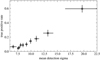 |
Fig. 4. Empirical true positive rate of matched filtering after checking about 1200 stars with detected emission lines. Each bin contains 90 stars and the errorbars in x-direction contain the central 1σ interval of the detection significance per bin. |
Table A.2 lists all stars with spectra containing valid emission lines that we found in our survey. This table also gives the original ID used in the ACS catalogue in column “ACS ID”. The columns “dC” lists the projected distance to the respective cluster centre. The table also contains our estimate whether the star is a likely cluster member in column “mem.?”. In contrast to Kamann et al. (2018), this estimate is based on radial velocities only. Column “vrad?” contains an indicator whether the star shows variations in its radial velocity based on the method described in Giesers et al. (2019). We converted the probability of variability calculated in Giesers et al. (2019) in the following way: p < 0.15: not variable, p > 0.85: variable, 0.15 < p < 0.86: unsure (?). Blank fields indicate insufficient data. We expect a false positive rate of 15%. Cross-matches with other catalogues and papers are given in column “Ident.” with the corresponding reference in column “Ref.”. The column “dX” contains the separation to the next Chandra X-ray source (Evans et al. 2010), if it is less than the positional uncertainties of the X-ray source. Background galaxies are listed in Table 3.
Positions and redshifts of background galaxies with emission lines.
Choice of V filter for each cluster used in this paper.
4.2. Cataclysmic variables
As described above, CVs are binary systems consisting of a hot, compact white dwarf and a dwarf star in a close orbit. Only ten CVs have been confirmed by spectroscopy in the whole globular cluster system of the Milky Way (Knigge 2012; Webb & Servillat 2013). Most CV candidates identified by photometry are not bright enough to be observed with MUSE and our relatively short exposure times. For example, Rivera Sandoval et al. (2018) lists R625 magnitudes for 21 CV candidates in NGC 104 of which only four are brighter than 20 mag.
4.2.1. Known CVs and confirming CV candidates
We find nine CVs, of which seven are either previously spectroscopically confirmed CVs or candidates. The normalised MUSE spectra of several CVs including the previously unknown ones are shown in Fig. 5. Characteristic broad Balmer emission lines of Hα and Hβ are clearly visible in all spectra, as well as He I emission.
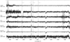 |
Fig. 5. Normalised spectra of known cataclysmic variables AKO9, CX1, CX2, CV1, of the new CVs in NGC 6681 and NGC 7099, and of the CV underlying the Nova T Sco in 1860. All spectra are detected by their broad Balmer emission lines, they also show He I emission. The spectrum shown for AKO9 was created by combining several observed spectra. |
One of them, CX1 in NGC 6218 was detected as an X-ray source with optical counterpart and classified as a CV by Lu et al. (2009) who consider it to be a member of the cluster based on its X-ray luminosity. We find that its optical counterpart is not the star marked in their finding chart but rather the star directly to the east with a F606W magnitude of 20.8. With this new counterpart, we can confirm that CX1 is indeed a CV.
We do not see the characteristic broad Balmer emission lines for a CV in any spectrum of W56/X6 in NGC 104 which was classified as a CV in Heinke et al. (2005). However, the spectra show a Hα absorption line that is less deep than our spectral model predicts. Since this is not clearly a CV, we do not include it in our discussion in Sect. 5.1.
4.2.2. Nova T Scorpii
In 1860, a classical nova in NGC 6093 was observed by Pogson (1860), Nova T Scorpii. Both Shara & Drissen (1995) and Dieball et al. (2010) looked for the underlying CV using near- and far-UV observations and they found a UV bright source at the right spatial position. Using the finding charts in Dieball et al. (2010), we can identify their source 2129 with ACS ID 44184 (F336W−F438W = −0.1, F438W = 18.5, Piotto et al. 2015; Soto et al. 2017). This star was independently detected by our algorithm because of its broad Hα emission in several of its ten spectra observed with MUSE. A visual inspection shows that also Hβ and a weak He I emission are present and variable. The Hα and Hβ lines seem to switch between emission and absorption. However, as ACS ID 44184 is located on the lower RGB in the optical CMD, the CV has either a giant donor star or it is not resolved in the HST photometry but instead blended with a unrelated star.
4.2.3. New cataclysmic variables
Additionally to the seven known CVs, we find two more stars with very similar emission lines, indicating that these two stars are CVs as well. One new CV is close to the centre of NGC 7099 with a distance of 11″ and a F606W magnitude of 20.3 in the ACS catalogue (ACS ID 23423). Based on its position close to an X-ray source and its blue U − V colour, Lugger et al. (2007) identified this star as a possible CV candidate (source C). However, it is not included as a CV in the CVSGGC, which is why we list it as a new CV here.
The new CV in NGC 6681 (ACS ID 19706) has a distance of 27″ to the cluster centre and a F606W magnitude of 22.7. The spectra of the new and known CVs are shown in Fig. 5. Both new CVs are close (0.13 and 0.25″, respectively) to a Chandra X-ray source listed in the November 2017 pre-release of the Chandra Source Catalog Release 2.0 (Evans et al. 2010). Although NGC 6681 was observed with HST in the UV (see e.g. Massari et al. 2013) and with the Chandra X-ray observatory (Pooley 2007; Dieball 2008), no articles about CVs in this cluster have been published.
Are these CVs actually part of their respective cluster? In general, we use the radial velocity and metallicity to determine if a star is a member of a globular cluster or a field star. The standard spectral fit failed to determine reliable radial velocities or metallicities from the spectra of the new CVs. We used a Gaussian fit to the Hα line to estimate the radial velocity for each CV, including the known CVs. The velocities differ from the cluster values by up to 300 km s−1. This could be because the emission lines in some cases seem to have a more complex, that is non-Gaussian, shape, or because of intrinsically high velocity variations due to the orbital motions, or possibly because of eclipses of the accretion disc as observed for AKO9 (Knigge et al. 2003).
We assume that CVs in GCs are spatially distributed in the same way as all other stars in a GC. In the simulations of Belloni et al. (2019) CVs are either distributed more centrally or in the same way as main-sequence stars, depending on the relation time of the GCs. With this property of CVs we can also use Bayes factors to decide between the two hypotheses A ≡ “CV is a cluster member” and B ≡ “CV is not a cluster member”. To calculate the factors we made use of the spatial distribution and membership probability derived from the observed radial velocity and metallicity of all the other stars observed with MUSE in the same field of view (see Kamann et al. 2018 for details). The distances of the new CVs to the respective cluster centre are about 1/6 of the half-light radius (NGC 7099) and 2/3 (NGC 6681) when the values from Harris (1996) are used. In the MUSE field of view (FoV) of NGC 7099 96% of all stars are cluster members; this leaves about 4% non-members. Of all member stars, 8% are closer to the cluster centre than the CV we consider, while the remaining 92% are farther away. Thus, the likelihood of being a member star and at the same separation from the cluster centre or even closer is pA = 0.074. As for non-members, 10% lie closer to the centre than the CV, and 90% are farther away. This gives pB = 0.004. The Bayes factor is pA/pB ≈ 18, which means that the positions of the CV provide evidence in favour of hypothesis A. The same analysis for the CV that may be associated with NGC 6681 gives a Bayes factor of pA/pB ≈ 13. Here, 92% are member stars, of which two third lie closer to the centre than the CV. Of the 8% non-members, 55% lie closer to the centre. According to the interpretation of Jeffreys (1998, p. 432), Bayes factors between 10 and 103/2 provide strong evidence in favour of hypothesis A. In conclusion, the positions of the CVs and all the other stars in the MUSE FoV strongly suggest that both CVs are members of the respective cluster.
4.3. Optical counterpart of M62-VLA1
Several stellar mass black holes or candidates are known in globular clusters, including three in NGC 3201 (Giesers et al. 2018, 2019), M22-VLA1 and -VLA2 in NGC 6656 (Strader et al. 2012), and M62-VLA1 in NGC 6266 (Chomiuk et al. 2013). The black-hole candidates in NGC 3201 were discovered by Giesers et al. (2018, 2019) using variations in the radial velocities of their visible companions observed with MUSE. These discoveries demonstrate that MUSE observations can be used to detect stellar exotica in GCs.
The black-hole candidate M62-VLA1 is close to the centre of NGC 6266 and was discovered by Strader et al. (2012) using radio and X-ray observations. It is likely to be part of a binary system with a star on the lower RGB, which the authors identified in HST images very close to their radio source. Our emission-line search found the optical counterpart of this black hole because of its Hα emission line. Both the position of this star and the counterpart reported in Strader et al. (2012) match, as well as the location in the colour-magnitude diagram. This star was observed several times with MUSE in 2015 and again in 2018 with varying S/N. The spectra with the highest S/N show a Hα emission line which seem to vary between observations. These variations in the Hα region are shown in Fig. 6 where the shape of the emission line changes within tens of minutes. We need more observations to determine reliable orbital parameters for this system similarly to the black holes and the 92 other binary systems in NGC 3201 (Giesers et al. 2019).
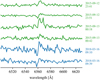 |
Fig. 6. Hα region of multiple spectra of the likely companion of the black-hole candidate M62-VLA1. This part of the spectrum is variable on the timescale of minutes. |
4.4. Red stragglers and sub-subgiants
Red stragglers (RS) and sub-subgiants (SSG) are stars in globular clusters that occupy the region redwards of the RGB or below the subgiant branch in the CMD. Since stellar evolution theory predicts these regions to be empty, their existence needs to be explained by more complicated formation theories (Geller et al. 2017a,b; Leiner et al. 2017). In addition to their unusual location in the CMD, RS are X-ray and Hα emitters, photometrically variable and mostly radial-velocity binaries (Geller et al. 2017a). As expected, several detected emission-line stars fall into the CMD region occupied by RS (four stars) and SSG (12 stars, see column “ID” in Table A.2). In particular, we detected the RS binary in NGC 6254 discovered by Shishkovsky et al. (2018) which is also a source of radio and X-ray radiation. A similar case is a star (ACS ID 40733) in the RS region of NGC 6541 which has a very broad and variable Hα emission, and it is close to an X-ray source ( ). Of the eleven SSG that show Hα emission and are probable cluster members, eight are close to an X-ray source, eight show variations in their radial velocities, and seven SSG are both close to an X-ray source and have radial velocity variations. All four RS with Hα emission are members of their respective cluster, three are close to an X-ray source and those three RS also show radial velocity variations. We did not detect variability in the radial velocities of the fourth RS and it is not associated with an X-ray source. These correlations fit the general characteristics of SSG and RS as described in Geller et al. (2017a). Orbital parameters for several SSG systems in NGC 3201, including the Hα emitters discovered here, are presented in Giesers et al. (2019).
4.5. Pulsating variables
About 40% of all emission-line stars found in this survey are already known pulsating variable stars including W Viriginis variables, slow irregular variables, long-period variables, semiregular variables, and RR Lyrae variables. Spectra of these stars show constant or variable Hα and sometimes Hβ emission fluxes.
Since the work of Struve (1947) it is known that spectra of RR Lyrae stars have a varying, weak emission component in several Hydrogen lines. Figure 7 shows two spectra of the RR Lyrae star V90 in NGC 3201 as an example of variable emission lines. The two spectra were observed roughly 24 h apart and only the earlier one shows Hα and Hβ emission lines. The flux profiles are very similar to the first or second apparition of the RR Lyr variable X Ari shown Gillet & Fokin (2014) in Fig. 1. The variable star V13 and possibly also V190 in NGC 6266 are currently classified as RR Lyrae stars in the literature. However, their spectra show very strong Hα and Hβ emission lines, similar to those of W Viriginis variables.
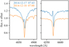 |
Fig. 7. Two spectra of the RR Lyrae star NGC 3201-V90 (CVSGGC) observed approximately 24 h apart show very different Balmer profiles. Hα and Hβ emission is only observed in one of the spectra, but not in the other one. |
4.6. Known nebulae
There are four known planetary nebulae (PNe) in the whole globular cluster system of the Milky Way. These are Ps 1 in NGC 7078 (Pease 1928), GJJC-1 in NGC 6656 (Gillett et al. 1989), JaFu-1 in Pal 6, and JaFu-2 in NGC 6441 (both Jacoby et al. 1997).
The most successful and also largest survey of PNe in globular clusters is the one from Jacoby et al. (1997), who used the on-band/off-band technique at the [O III] line at 5007 Å on 133 globular clusters. With this survey, they doubled the number of known PNe in GCs from two to four.
Of the four globular clusters with known PNe, Pal 6 is not included in our sample of GCs. Although our survey covers NGC 6656, GJJC-1 is not inside the MUSE FoV because of its position inside the cluster. This leaves Ps 1 and JaFu-2 for which we provide flux maps and spectra. Figure 8 shows [O III] maps of the two PNe side-by-side, the PN spectra are shown in Fig. 9. The spectra were extracted with a relatively large circular aperture covering the whole nebula. Although the nebulae are not HST point sources and, accordingly, we did not automatically extract a spectrum at their positions, the detection algorithm finds the nebular emission lines. This is because their emission flux contaminated the otherwise purely stellar spectra of dozens of nearby stars as its high spatial variability is not accounted for in the extraction.
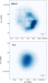 |
Fig. 8. Flux maps of the two known planetary nebulae in our sample: JaFu-2 (top) in NGC 6441 and Ps 1 (bottom) in NGC 7078. Shown is the [O III]λ5007 flux after the stellar background has been subtracted. |
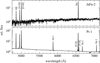 |
Fig. 9. Spectra of JaFu-2 (top) and Ps 1 (bottom). Prominent emission lines of Hydrogen, He I, [N II], and [O III] are labelled. |
In addition to these two planetary nebulae, we detected a nova remnant in NGC 6656 which is described in detail in Göttgens et al. (2019). However, we did not find any additional nebulae in our observations. We checked this null-result by stacking cubes from different observations to increase our sensitivity. We used the on-band/off-band technique around Hα to search for extended emitting regions and did not find any nebula.
4.7. Galaxies
For each spectrum, we used the full list of emission-line candidates and their wavelengths to check if they correspond to a list of typical galactic emission lines, assuming they all have the same redshift. Using this method, we find 21 background galaxies that contaminate spectra we have extracted at known stellar positions in observations of several GCs (see Table 3). Since these spectra contain the stellar Hα absorption line, we conclude that these are indeed blended spectra of a star and a background galaxy. The spectra were identified by their prominent emission lines of Hydrogen and ionised Oxygen, as shown in Fig. 10 for three examples. We detected emission lines corresponding to restframe wavelengths of 3727 Å from [O II], of 4959 Å and 5007 Å from [O III], and Hβ and Hα emission. Table 3 lists the position, the redshift calculated from the emission lines, and the projected angular separation to the cluster centre for each galaxy. Because of the low [N II] to Hα flux, all galaxies fall into the region occupied by starburst galaxies in the BPT diagram (Baldwin et al. 1981; Veilleux & Osterbrock 1987), except for one galaxy behind NGC 6752 at z = 0.364 which lies at the border of Seyfert galaxies and LINER. Deeper photometric observations of the fields containing the new galaxies may identify the counterparts which could be used to convert relative stellar proper motions into absolute proper motions, as done for NGC 6681 using HST images (Massari et al. 2013). These serendipitous discoveries resemble the one reported by Bedin et al. (2019), who found a dwarf spheroidal galaxy behind the globular cluster NGC 6752 using HST photometry. The fact that a galaxy lies very close to the core of the core-collapsed cluster NGC 7099 shows our capability to look through the GCs.
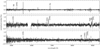 |
Fig. 10. Normalised residuals of stellar spectra that contain extragalactic emission lines including from [O II], [O III], and H I. Redshifts determined from these lines are z = 0.05, 0.36 and 0.737, respectively. Top and bottom panels: starburst galaxy, while middle panel: AGN. |
4.8. Unidentified sources
We find several emission-line stars that lie close to known X-ray sources. As a reference, we used the November 2017 pre-release of the Chandra Source Catalog Release 2.0 (Evans et al. 2010), which includes positions and error ellipses (including astrometric uncertainties) for X-ray sources in all but two clusters in our survey (NGC 6254 and NGC 6624). Based on the source positions and the associated errors, we estimated that there is no physical relation between a star and an X-ray source if their distance is > 1″. In general, multiple stars have a distance > 1″ to an X-ray source which prohibits a unique identification of the optical counterpart. However, because both emission-line sources and X-ray sources are rare objects in globular clusters, we indicate if an X-ray source is close in the Table A.2.
As indicated in Table A.2, some stars show variable Hα emission wings or asymmetric absorption. In the case of giant stars, these features could point to chromospheric activity or mass motions (e.g. Cohen 1976; Cacciari et al. 2004; Meszaros et al. 2008).
5. Discussion and conclusions
5.1. Completeness of the extraction of stellar sources
There are two steps in the detection of emission-line sources in MUSE data that influence how many existing sources can be found: the extraction completeness and the efficiency of matched filtering. We discuss only the first one here, the second one was described in Sect. 3.3.
The extraction completeness is the ratio of ACS catalogue sources for which a spectrum can be extracted from the MUSE datacube to all sources in the MUSE field of view. Figure 11 shows the dependence of our extraction completeness for all clusters taking all spectra with a S/N better than five into account. An extraction completeness of 100% does not mean that we have a spectrum of all stars in our FoV but only of those listed in the ACS catalogue. This is an important distinction for low brightness stars in the central few arcseconds of core-collapsed clusters, such as NGC 7078. Thus we expect that the completeness depends not only on the brightness of a star but also on its position relative to the cluster centre (see Fig. A.1).
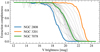 |
Fig. 11. Spectral extraction completeness (S/N > 5) for all clusters with respect to the ACS catalogue as a function of brightness (filters are listed in Table 4). Each grey curve represents a single cluster, the curves for NGC 2808, NGC 3201, and NGC 7078 are highlighted. Since the completeness mainly depends on the stellar density, it also depends on the radial distance to the cluster centre (see Fig. A.1). |
We estimate the extraction completeness for different magnitudes and for three regions: the whole FoV, the central 10″, the intermediate region from 10″ to 60″ and the remaining outer regions. Figure A.1 shows how our extraction completeness depends on the brightness of the star and its position in the case of NGC 7078. In general we see a completeness of close to 100% for bright stars throughout the cluster. The crowded cluster centre hinders the extraction of faint sources and the completeness starts to drop below 50% for magnitudes between 18 and 19 mag for most clusters.
5.2. Do we find enough CVs?
Massive globular clusters are expected to host about 200 CVs (Ivanova et al. 2006; Knigge 2012). However, the cluster with the most CV candidates, as determined by UV and optical photometry and X-ray data, is NGC 104 with 43 CVs (Rivera Sandoval et al. 2018). In contrast, the number of spectroscopically confirmed CVs is much lower: only ten CVs have been confirmed by spectroscopy in the whole globular cluster system of the Milky Way (Knigge 2012; Webb & Servillat 2013). We add seven CVs to this list, including two newly detected CVs. CVs in globular clusters are hard to observe by spectroscopy because of the low brightness of the secondary component and crowding. We expect to find dwarf novae (DNe), a subtype of CVs, because they have spectra with emission lines in quiescence (Clarke et al. 1984; Warner 1995) and observations show that most CVs are DNe (Knigge et al. 2011). Is our number of CV detections consistent with the prediction? To answer this question, we used the average CV brightness distribution from MOCCA simulations of globular clusters (Belloni et al. 2016). We did not consider the effects of incomplete spatial coverage in our survey, because most CVs are expected to be located inside the half-mass radius of the respective cluster (Belloni et al. 2016, but also see Belloni et al. 2019). For each cluster, we drew samples from this distribution and used our completeness function and a detection probability of 80% (Sect. 3.3) to estimate the number of CVs for which we should have extracted spectra (see Table A.1). Since the clusters differ in their structural parameters and Belloni et al. (2016) give a CV brightness distribution for an average globular cluster, the number of CVs for each individual cluster is probably not meaningful. The total number of expected CV detections using the model of Belloni et al. (2016) in our sample is 10 ± 2, which is consistent with our number of nine detected CVs.
The step that restricts the overall completeness for CVs the most is the extraction completeness at magnitudes of 22 and below. This could be improved with longer observations using the narrow-field mode (NFM) of MUSE, which will offer a much higher spatial sampling in a smaller FoV.
5.3. Exclusion of more PNe
While the limiting fluxes given in Table 2 are, if interpreted strictly, only valid for emission in stellar spectra, we can rule out any large diffuse source of Hα emission lines in our fields of view. Any nebula or other diffuse source of emission would need to overlap with at least some stars of which we extracted spectra. In the same way we easily detected JaFu-2, Ps 1, and the nova remnant in NGC 6656 (Göttgens et al. 2019), these contaminated spectra would have been found.
There are still some possible but unlikely ways a hypothetical PNe could be hidden in a GC: It could be very small so that it only contaminates a few stars, ideally of low brightness. In this case, we might not extract a spectrum for them. The maximum size of this nebula cannot be large, considering the high density of sources for which we can extract spectra. Another possibility is a nebula with very faint Hα emission that would have to be much fainter than the known ones because those were easily found with our detection method.
However, it is still possible that more nebulae similar to the nova in NGC 6656 lie outside the area covered by our survey. In this case, it has to be in a region of relatively high stellar density where it cannot be detected by photometric surveys.
6. Summary
We analysed data from our MUSE survey of 26 Galactic globular clusters, looking for signs of emission-line objects. Taking advantage of previous work on the same data, including data reduction, spectra extraction, and spectral analysis, we find 156 emission-line stars and several non-stellar emission-line sources. By assuming a Gaussian emission-line shape and using matched filtering, we detected this shape in the residuals generated during a full spectrum fit to the observed spectra. Since this generated many potentially interesting emission-line candidates, we use a threshold to select only the most promising candidates and checked them visually. We did not use external catalogues to search for known sources in our data, but we used them to validate and categorise our findings. We find two new cataclysmic variables, many known pulsating variable stars, and several unidentified emission-line stars close to known X-ray sources. The total number of CVs detected in this survey is consistent with numerical simulations when our spectral extraction completeness is taken into account. In addition to stellar emission-line sources, we also find 20 previously unknown starburst galaxies and one AGN in the background with redshifts from 0.05 to 0.74.
ESO Programme IDs: 094.D-0142, 095.D-0629, 096.D-0175, 097.D-0295, 098.D-0148, 099.D-0019, 0100.D-0161, 0101.D-0268, and 0102.D-0270.
Acknowledgments
We want to thank R. Terlevich for his helpful comment about the emission lines in the PN spectra. FG, SK, and SD acknowledge support from the German Research Foundation (DFG) through projects KA 4537/2-1 and DR 281/35-1. SK gratefully acknowledges funding from a European Research Council consolidator grant (ERC-CoG-646928- Multi-Pop). PMW, SK, SD, and BG also acknowledge support from the German Ministry for Education and Science (BMBF Verbundforschung) through projects MUSE-AO, grants 05A14BAC and 05A14MGA, and MUSE-NFM, grants 05A17MGA and 05A17BAA. Based on observations made with ESO Telescopes at the La Silla Paranal Observatory under programme IDs 094.D-0142, 095.D-0629, 096.D-0175, 097.D-0295, 098.D-0148, 099.D-0019, 0100.D-0161, 0101.D-0268, and 0102.D-0270. Also based on observations made with the NASA/ESA Hubble Space Telescope, obtained from the data archive at the Space Telescope Science Institute. STScI is operated by the Association of Universities for Research in Astronomy, Inc. under NASA contract NAS 5-26555.
References
- Abbott, B., Abbott, R., Abbott, T., et al. 2016, Phys. Rev. Lett., 116, 061102 [Google Scholar]
- Albrow, M. D., Gilliland, R. L., Brown, T. M., et al. 2001, ApJ, 559, 1060 [NASA ADS] [CrossRef] [Google Scholar]
- Anderson, J., Sarajedini, A., Bedin, L. R., et al. 2008, AJ, 135, 2055 [NASA ADS] [CrossRef] [Google Scholar]
- Askar, A., Sedda, M. A., & Giersz, M. 2018, MNRAS, 478, 1844 [NASA ADS] [CrossRef] [Google Scholar]
- Bacon, R., Accardo, M., Adjali, L., et al. 2010, in Ground-based and Airborne Instrumentation for Astronomy III, Int. Soc. Opt. Photon., 7735, 773508 [CrossRef] [Google Scholar]
- Bacon, R., Conseil, S., Mary, D., et al. 2017, A&A, 608, A1 [NASA ADS] [CrossRef] [EDP Sciences] [Google Scholar]
- Baldwin, J. A., Phillips, M. M., & Terlevich, R. 1981, PASP, 93, 5 [NASA ADS] [CrossRef] [EDP Sciences] [Google Scholar]
- Bassa, C., Pooley, D., Homer, L., et al. 2004, ApJ, 609, 755 [NASA ADS] [CrossRef] [Google Scholar]
- Bedin, L. R., Salaris, M., Rich, R. M., et al. 2019, MNRAS, 484, L54 [NASA ADS] [Google Scholar]
- Belloni, D., Giersz, M., Askar, A., Leigh, N., & Hypki, A. 2016, MNRAS, 462, 2950 [NASA ADS] [CrossRef] [Google Scholar]
- Belloni, D., Giersz, M., Rivera Sandoval, L. E., Askar, A., & Ciecielag, P. 2019, MNRAS, 483, 315 [NASA ADS] [CrossRef] [Google Scholar]
- Cacciari, C., Bragaglia, A., Rossetti, E., et al. 2004, A&A, 413, 343 [NASA ADS] [CrossRef] [EDP Sciences] [Google Scholar]
- Campos, F., Pelisoli, I., Kamann, S., et al. 2018, MNRAS, 481, 4397 [NASA ADS] [CrossRef] [Google Scholar]
- Chomiuk, L., Strader, J., Maccarone, T. J., et al. 2013, ApJ, 777, 69 [NASA ADS] [CrossRef] [Google Scholar]
- Clarke, J. T., Capel, D., & Bowyer, S. 1984, ApJ, 287, 845 [NASA ADS] [CrossRef] [Google Scholar]
- Clement, C. 2017, EPJ Web Conf., 152, 01021 [Google Scholar]
- Clement, C. M., Muzzin, A., Dufton, Q., et al. 2001, AJ, 122, 2587 [NASA ADS] [CrossRef] [Google Scholar]
- Cohen, J. G. 1976, ApJ, 203, L127 [NASA ADS] [CrossRef] [Google Scholar]
- Cool, A. M., Haggard, D., Arias, T., et al. 2013, ApJ, 763, 126 [NASA ADS] [CrossRef] [Google Scholar]
- Dieball, A. 2008, Chandra Proposal 10300600 [Google Scholar]
- Dieball, A., Long, K. S., Knigge, C., Thomson, G. S., & Zurek, D. R. 2010, ApJ, 710, 332 [NASA ADS] [CrossRef] [Google Scholar]
- Evans, I. N., Primini, F. A., Glotfelty, K. J., et al. 2010, ApJS, 189, 37 [NASA ADS] [CrossRef] [EDP Sciences] [Google Scholar]
- Geller, A. M., Leiner, E. M., Bellini, A., et al. 2017a, ApJ, 840, 66 [NASA ADS] [CrossRef] [Google Scholar]
- Geller, A. M., Leiner, E. M., Chatterjee, S., et al. 2017b, ApJ, 842, 1 [NASA ADS] [CrossRef] [Google Scholar]
- Giesers, B., Dreizler, S., Husser, T.-O., et al. 2018, MNRAS, 475, L15 [NASA ADS] [CrossRef] [Google Scholar]
- Giesers, B., Kamann, S., Dreizler, S., et al. 2019, A&A, in press, https://doi.org/10.1051/0004-6361/201936203 [Google Scholar]
- Gillet, D., & Fokin, A. B. 2014, A&A, 565, A73 [NASA ADS] [CrossRef] [EDP Sciences] [Google Scholar]
- Gillett, F. C., Jacoby, G. H., Joyce, R. R., et al. 1989, ApJ, 338, 862 [NASA ADS] [CrossRef] [Google Scholar]
- Göttgens, F., Weilbacher, P. M., Roth, M. M., et al. 2019, A&A, 626, A69 [NASA ADS] [CrossRef] [EDP Sciences] [Google Scholar]
- Harris, W. E. 1996, AJ, 112, 1487 [NASA ADS] [CrossRef] [Google Scholar]
- Heinke, C. O., Grindlay, J. E., Edmonds, P. D., et al. 2003, ApJ, 598, 516 [NASA ADS] [CrossRef] [Google Scholar]
- Heinke, C. O., Grindlay, J. E., Edmonds, P. D., et al. 2005, ApJ, 625, 796 [NASA ADS] [CrossRef] [Google Scholar]
- Herenz, E. C., & Wisotzki, L. 2017, A&A, 602, A111 [NASA ADS] [CrossRef] [EDP Sciences] [Google Scholar]
- Husser, T.-O., Wende-von Berg, S., Dreizler, S., et al. 2013, A&A, 553, A6 [NASA ADS] [CrossRef] [EDP Sciences] [Google Scholar]
- Husser, T.-O., Kamann, S., Dreizler, S., et al. 2016, A&A, 588, A148 [NASA ADS] [CrossRef] [EDP Sciences] [Google Scholar]
- Ivanova, N., Heinke, C. O., Rasio, F. A., et al. 2006, MNRAS, 372, 1043 [NASA ADS] [CrossRef] [Google Scholar]
- Jacoby, G. H., Morse, J. A., Fullton, L. K., Kwitter, K. B., & Henry, R. B. C. 1997, AJ, 114, 2611 [NASA ADS] [CrossRef] [Google Scholar]
- Jacoby, G. H., Marco, O. D., Davies, J., et al. 2017, ApJ, 836, 93 [NASA ADS] [CrossRef] [Google Scholar]
- Jeffreys, H. 1998, The Theory of Probability (Oxford: Oxford University Press) [Google Scholar]
- Kaluzny, J., Rozyczka, M., Thompson, I. B., et al. 2016, Acta Astron., 66, 31 [NASA ADS] [Google Scholar]
- Kamann, S., Wisotzki, L., & Roth, M. M. 2013, A&A, 549, A71 [NASA ADS] [CrossRef] [EDP Sciences] [Google Scholar]
- Kamann, S., Husser, T.-O., Dreizler, S., et al. 2018, MNRAS, 473, 5591 [NASA ADS] [CrossRef] [Google Scholar]
- Knigge, C. 2012, Mem. Soc. Astron. It., 83, 549 [NASA ADS] [Google Scholar]
- Knigge, C., Zurek, D. R., Shara, M. M., Long, K. S., & Gilliland, R. L. 2003, ApJ, 599, 1320 [NASA ADS] [CrossRef] [Google Scholar]
- Knigge, C., Baraffe, I., & Patterson, J. 2011, ApJS, 194, 28 [NASA ADS] [CrossRef] [Google Scholar]
- Kremer, K., Ye, C. S., Chatterjee, S., Rodriguez, C. L., & Rasio, F. A. 2018, ApJ, 855, L15 [NASA ADS] [CrossRef] [Google Scholar]
- Kunder, A., Stetson, P. B., Catelan, M., Walker, A. R., & Amigo, P. 2013, AJ, 145, 33 [NASA ADS] [CrossRef] [Google Scholar]
- Lebzelter, T., & Wood, P. R. 2016, A&A, 585, A111 [NASA ADS] [CrossRef] [EDP Sciences] [Google Scholar]
- Leiner, E., Mathieu, R. D., & Geller, A. M. 2017, ApJ, 840, 67 [NASA ADS] [CrossRef] [Google Scholar]
- Lu, T.-N., Kong, A. K. H., Bassa, C., et al. 2009, ApJ, 705, 175 [NASA ADS] [CrossRef] [Google Scholar]
- Lugger, P. M., Cohn, H. N., Heinke, C. O., Grindlay, J. E., & Edmonds, P. D. 2007, ApJ, 657, 286 [NASA ADS] [CrossRef] [Google Scholar]
- Lugger, P. M., Cohn, H. N., Cool, A. M., Heinke, C. O., & Anderson, J. 2017, ApJ, 841, 53 [NASA ADS] [CrossRef] [Google Scholar]
- Massari, D., Bellini, A., Ferraro, F. R., et al. 2013, ApJ, 779, 81 [NASA ADS] [CrossRef] [Google Scholar]
- Meszaros, S., Dupree, A. K., & Szentgyorgyi, A. 2008, AJ, 135, 1117 [NASA ADS] [CrossRef] [Google Scholar]
- Ochsenbein, F., Bauer, P., & Marcout, J. 2000, A&AS, 143, 23 [NASA ADS] [CrossRef] [EDP Sciences] [Google Scholar]
- Pease, F. G. 1928, PASP, 40, 342 [NASA ADS] [CrossRef] [Google Scholar]
- Piotto, G., Milone, A. P., Bedin, L. R., et al. 2015, AJ, 149, 91 [NASA ADS] [CrossRef] [Google Scholar]
- Pogson, N. 1860, MNRAS, 21, 32 [NASA ADS] [CrossRef] [Google Scholar]
- Pooley, D. 2007, Chandra Proposal 09300101 [Google Scholar]
- Pooley, D., Lewin, W. H. G., Homer, L., et al. 2002, ApJ, 569, 405 [NASA ADS] [CrossRef] [Google Scholar]
- Ransom, S. M. 2007, Proc. Int. Astron. Union, 3, 291 [CrossRef] [Google Scholar]
- Rivera Sandoval, L. E., van den Berg, M., Heinke, C. O., et al. 2018, MNRAS, 475, 4841 [NASA ADS] [CrossRef] [Google Scholar]
- Roth, M. M., Sandin, C., Kamann, S., et al. 2018, A&A, 618, A3 [NASA ADS] [CrossRef] [EDP Sciences] [Google Scholar]
- Sarajedini, A., Bedin, L. R., Chaboyer, B., et al. 2007, AJ, 133, 1658 [NASA ADS] [CrossRef] [Google Scholar]
- Shara, M. M., & Drissen, L. 1995, ApJ, 448, 203 [NASA ADS] [CrossRef] [Google Scholar]
- Shishkovsky, L., Strader, J., Chomiuk, L., et al. 2018, ApJ, 855, 55 [NASA ADS] [CrossRef] [Google Scholar]
- Soto, M., Bellini, A., Anderson, J., et al. 2017, AJ, 153, 19 [NASA ADS] [CrossRef] [Google Scholar]
- Strader, J., Chomiuk, L., Maccarone, T. J., Miller-Jones, J. C. A., & Seth, A. C. 2012, Nature, 490, 71 [NASA ADS] [CrossRef] [Google Scholar]
- Struve, O. 1947, PASP, 59, 192 [NASA ADS] [CrossRef] [Google Scholar]
- Veilleux, S., & Osterbrock, D. E. 1987, ApJS, 63, 295 [NASA ADS] [CrossRef] [Google Scholar]
- Vio, R., & Andreani, P. 2016, A&A, 589, A20 [NASA ADS] [CrossRef] [EDP Sciences] [Google Scholar]
- Warner, B. 1995, Cataclysmic Variable Stars, Cambridge Astrophysics (Cambridge, UK: Cambridge University Press), 126 [CrossRef] [Google Scholar]
- Webb, N. A., & Servillat, M. 2013, A&A, 551, A60 [NASA ADS] [CrossRef] [EDP Sciences] [Google Scholar]
- Webb, N. A., Serre, D., Gendre, B., et al. 2004, A&A, 424, 133 [NASA ADS] [CrossRef] [EDP Sciences] [Google Scholar]
- Weilbacher, P. M., Streicher, O., Urrutia, T., et al. 2012, in Software and Cyberinfrastructure for Astronomy II, Int. Soc. Opt. Photon., 8451, 84510B [CrossRef] [Google Scholar]
- Weilbacher, P. M., Streicher, O., Urrutia, T., et al. 2014, in Astronomical Data Analysis Software and Systems XXIII, eds. N. Manset, & P. Forshay, ASP Conf. Ser., 485, 451 [NASA ADS] [Google Scholar]
- Wendt, M., Husser, T.-O., Kamann, S., et al. 2017, A&A, 607, A133 [NASA ADS] [CrossRef] [EDP Sciences] [Google Scholar]
- Wenger, M., Ochsenbein, F., Egret, D., et al. 2000, A&AS, 143, 9 [NASA ADS] [CrossRef] [EDP Sciences] [Google Scholar]
Appendix A: Completeness
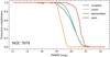 |
Fig. A.1. Spectral extraction completeness in NGC 7078 relative to the ACS catalogue. For this cluster, we reach a completeness of 50% at a magnitude of 17, 20, and 21.5 for the central region (innermost 10″), an intermediate region (between 10″ and 60″), and the outer regions (outside 60″), respectively. |
Number of expected CVs in each cluster using the brightness distribution from Belloni et al. (2016).
Stars with spectra containing significant emission lines.
All Tables
Limiting fluxes for all clusters, calculated using a broad emission line (40 Å) and also valid for narrow lines (see text).
Number of expected CVs in each cluster using the brightness distribution from Belloni et al. (2016).
All Figures
|
Fig. 1. Illustration of emission-line detection with matched filtering. Top: observed flux of V190 in NGC 6266 with Hα emission and the fitted spectral model. Bottom: Hα emission line is still present in the residuals, as well as an absorption line at 6700 Å which is only found in the models. The convolution with a Gaussian increases the emission line above the threshold calculated from the mean absolute deviation of the residuals. |
| In the text | |
|
Fig. 2. Fraction of simulated emission lines that are recovered with a filter width of 6 Å depending on the simulated line width. Only detections above a detection significance Ds > 7.5 are taken into account. |
| In the text | |
|
Fig. 3. Limiting flux for which 80% of sources will be detected as determined from simulated emission lines for different clusters as a function of brightness. Each grey curve represents a GC, the clusters NGC 104, NGC 3201, and NGC 5139 are highlighted. |
| In the text | |
|
Fig. 4. Empirical true positive rate of matched filtering after checking about 1200 stars with detected emission lines. Each bin contains 90 stars and the errorbars in x-direction contain the central 1σ interval of the detection significance per bin. |
| In the text | |
|
Fig. 5. Normalised spectra of known cataclysmic variables AKO9, CX1, CX2, CV1, of the new CVs in NGC 6681 and NGC 7099, and of the CV underlying the Nova T Sco in 1860. All spectra are detected by their broad Balmer emission lines, they also show He I emission. The spectrum shown for AKO9 was created by combining several observed spectra. |
| In the text | |
|
Fig. 6. Hα region of multiple spectra of the likely companion of the black-hole candidate M62-VLA1. This part of the spectrum is variable on the timescale of minutes. |
| In the text | |
|
Fig. 7. Two spectra of the RR Lyrae star NGC 3201-V90 (CVSGGC) observed approximately 24 h apart show very different Balmer profiles. Hα and Hβ emission is only observed in one of the spectra, but not in the other one. |
| In the text | |
|
Fig. 8. Flux maps of the two known planetary nebulae in our sample: JaFu-2 (top) in NGC 6441 and Ps 1 (bottom) in NGC 7078. Shown is the [O III]λ5007 flux after the stellar background has been subtracted. |
| In the text | |
|
Fig. 9. Spectra of JaFu-2 (top) and Ps 1 (bottom). Prominent emission lines of Hydrogen, He I, [N II], and [O III] are labelled. |
| In the text | |
|
Fig. 10. Normalised residuals of stellar spectra that contain extragalactic emission lines including from [O II], [O III], and H I. Redshifts determined from these lines are z = 0.05, 0.36 and 0.737, respectively. Top and bottom panels: starburst galaxy, while middle panel: AGN. |
| In the text | |
|
Fig. 11. Spectral extraction completeness (S/N > 5) for all clusters with respect to the ACS catalogue as a function of brightness (filters are listed in Table 4). Each grey curve represents a single cluster, the curves for NGC 2808, NGC 3201, and NGC 7078 are highlighted. Since the completeness mainly depends on the stellar density, it also depends on the radial distance to the cluster centre (see Fig. A.1). |
| In the text | |
|
Fig. A.1. Spectral extraction completeness in NGC 7078 relative to the ACS catalogue. For this cluster, we reach a completeness of 50% at a magnitude of 17, 20, and 21.5 for the central region (innermost 10″), an intermediate region (between 10″ and 60″), and the outer regions (outside 60″), respectively. |
| In the text | |
Current usage metrics show cumulative count of Article Views (full-text article views including HTML views, PDF and ePub downloads, according to the available data) and Abstracts Views on Vision4Press platform.
Data correspond to usage on the plateform after 2015. The current usage metrics is available 48-96 hours after online publication and is updated daily on week days.
Initial download of the metrics may take a while.