The full infrared spectrum of molecular hydrogen

E. Roueff; H. Abgrall; P. Czachorowski; K. Pachucki; M. Puchalski; J. Komasa

doi:10.1051/0004-6361/201936249

Home

All issues

Volume 630 (October 2019)

A&A, 630 (2019) A58

Full HTML

Open Access

Issue		A&A Volume 630, October 2019


Article Number		A58
Number of page(s)		5
Section		Atomic, molecular, and nuclear data
DOI		https://doi.org/10.1051/0004-6361/201936249
Published online		24 September 2019

A&A 630, A58 (2019)

The full infrared spectrum of molecular hydrogen^⋆

E. Roueff¹, H. Abgrall¹, P. Czachorowski², K. Pachucki², M. Puchalski³ and J. Komasa³

¹ Sorbonne Université, Observatoire de Paris, Université PSL, CNRS, LERMA, 92190 Meudon, France
e-mail: evelyne.roueff@obspm.fr
² Faculty of Physics, University of Warsaw, Pasteura 5, 02-093 Warsaw, Poland
³ Faculty of Chemistry, Adam Mickiewicz University, Uniwersytetu Poznańskiego 8, 61-614 Poznań, Poland

Received: 5 July 2019
Accepted: 15 August 2019

Abstract

Context. The high spectral resolution R ∼ 45 000 provided by IGRINS (Immersion Grating INfrared Spectrometer) at MacDonald Observatory and R ∼ 100 000 achieved by CRIRES (CRyogenic high-resolution InfraRed Echelle Spectrograph) at VLT (Very Large Telescope) challenges the present knowledge of infrared spectra.

Aims. We aim to predict the full infrared spectrum of molecular hydrogen at a comparable accuracy.

Methods. We take advantage of the recent theoretical ab initio studies on molecular hydrogen to compute both the electric quadrupole and magnetic dipole transitions taking place within the ground electronic molecular state of hydrogen.

Results. We computed the full infrared spectrum of molecular hydrogen at an unprecedented accuracy and derive for the first time the emission probabilities including both electric quadrupole (ΔJ = 0, ±2) and magnetic dipole transitions (ΔJ = 0) as well as the total radiative lifetime of each rovibrational state. Inclusion of magnetic dipole transitions increases the emission probabilities by factors of a few for highly excited rotational levels, which occur in the 3–20 μ range.

Key words: molecular data / molecular processes / infrared: general

^⋆

Full Table 2 is only available at the CDS via anonymous ftp to cdsarc.u-strasbg.fr (130.79.128.5) or via http://cdsarc.u-strasbg.fr/viz-bin/cat/J/A+A/630/A58

© E. Roueff et al. 2019

Open Access article, published by EDP Sciences, under the terms of the Creative Commons Attribution License (http://creativecommons.org/licenses/by/4.0), which permits unrestricted use, distribution, and reproduction in any medium, provided the original work is properly cited.

1. Introduction

Molecular hydrogen (H₂) is a symmetric molecule, which prohibits electric dipole transitions to occur within its X¹ ground electronic state. Then electric quadrupole and magnetic dipole transitions can take place, reciprocally submitted to ΔJ = 0, ±2 and ΔJ = 0 selection rules. Considerable attention has been paid to the ab initio studies of this simple molecule where the resolution of the one dimensional Schrödinger equation allows the energy spectrum of the ground electronic state to be derived, as described in the pioneering work by Kołos & Wolniewicz (1964). Various corrections have been further introduced in order to compare the theoretical ab initio values to the experimentally derived values by Dabrowski (1984) from the VUV (Vacuum Ultra-Violet) absorption and emission flash discharge spectra of H₂ in the Lyman and Werner bands. The rotation–vibration energy level measurements were derived for all vibrational levels v = 0−14, and a maximum rotational J value of J = 29 with a predicted accuracy of 0.1 cm⁻¹. These measurements challenged theoretical calculations as the discrepancy between experimentally derived values and theoretical calculations reached about 4 cm⁻¹ for highly excited rotational levels. An additional important step in the ground state energy determinations was provided by the study of the quadrupole infrared spectrum at the laboratory (Bragg et al. 1982; Jennings & Brault 1983), which provides level energy terms with an accuracy of about 0.001 cm⁻¹. These studies, which are limited to energy terms of low vibrational and rotational values, have prompted detailed fundamental ab initio studies of the H₂ spectrum where nonadiabatic, relativistic, quantum electrodynamic (QED) corrections are carefully introduced by Pachucki & Komasa (2009) and Komasa et al. (2011). In parallel, astrophysical observations in the infrared have allowed the detection of tens of highly H₂ excited emission rovibrational transitions occuring in so-called Photon dominated regions (PDRs) such as the Orion Bar (Kaplan et al. 2017) or NGC 7023 (Le et al. 2017) or in shocked regions such as the Orion KL outflow (Oh et al. 2016; Geballe et al. 2017) and Herbig-Haro objects (Pike et al. 2016). Forthcoming infrared facilities, such as CRIRES (CRyogenic high-resolution InfraRed Echelle Spectrograph) at VLT (Very Large Telescope) and JWST (James Webb Space Telescope) in space will allow the wavelength window and the sensitivity to be extended. We find that it is thus timely to provide the complete infrared spectrum of H₂ involving any possible transition linking all available rovibrational levels at the highest level of accuracy.

2. Infrared spectrum of ground state H₂

2.1. Quantum mechanical calculations of line positions

Individual energy levels and their wave functions were determined in the framework of the nonrelativistic quantum electrodynamics (NRQED; Caswell & Lepage 1986; Pachucki 2005). This theory is suitable for bound energy levels of atomic and molecular systems composed of light nuclei. Within this approach, the energy is expressed in the form of an expansion in powers of the fine structure constant α

(1)

where E⁽ⁱ⁾ is proportional to αⁱ and may contain powers of lnα. The subsequent terms of this expansion are commonly known as the nonrelativistic energy E⁽²⁾, the relativistic E⁽⁴⁾, the QED E⁽⁵⁾, and higher order E⁽ⁱ⁾, i > 5, corrections. Each term, in turn, can be expanded in the small electron-to-proton mass ratio m_e/M_P as implemented in the nonadiabatic perturbation theory (NAPT) by Pachucki & Komasa (2008, 2015). The nonrelativistic energy E⁽²⁾ is then obtained by solving the nonadiabatic radial Schrödinger equation composed of the Born–Oppenheimer, the adiabatic correction, and the nonadiabatic correction potentials (Pachucki & Komasa 2009). For H₂ these electronic potentials are known to the relative accuracy of 10⁻⁹ − 10⁻¹⁴ (Pachucki 2010; Pachucki & Komasa 2014, 2015), which enables the nonrelativistic dissociation energy of an individual level to be determined with the accuracy limited only by the missing higher order nonadiabatic corrections ∼(m_e/M_P)³. The latter have recently been found to be of the order of 10⁻⁴ − 10⁻⁵ cm⁻¹ (Pachucki & Komasa 2018).

The hydrogen molecule in its electronic ground state (X) accommodates 302 bound states¹. An apparent advantage of the NAPT approach is that once the necessary potentials are constructed all the energy levels can be obtained simultaneously. An alternative to the NAPT and significantly more accurate approach to the nonrelativistic energy has recently been developed by Pachucki & Komasa (2018). In this approach, the E⁽²⁾ of a selected energy level is evaluated directly in a four-body calculation without separation of electronic and nuclear movements. The accuracy of such calculations is limited by the current precision of the physical constants and amounts to 10⁻⁷ cm⁻¹ for the dissociation energy of an individual level. At present, for about one-fifth of all the bound levels much more accurate nonrelativistic energies are available.

The NAPT was also applied to evaluate the relativistic correction E⁽⁴⁾. The electronic relativistic potential for H₂ was determined with accuracy higher than 10⁻⁶ cm⁻¹ by Puchalski et al. (2017). Recently, Czachorowski et al. (2018) evaluated the leading order recoil ∼m_e/M_P correction to this potential so that currently its accuracy is limited by the unknown higher order terms ∼(m_e/M_P)² and is of the order of 10⁻⁶ cm⁻¹. The uncertainty introduced by the E⁽⁴⁾ term to the dissociation energy of a level is estimated as 10⁻⁶ cm⁻¹.

The QED term E⁽⁵⁾ was obtained from the electronic QED potential determined by Piszczatowski et al. (2009) and later refined by Puchalski et al. (2016, 2017). So far, no numerical values for the finite nuclear mass (i.e. recoil) correction to the QED potential are known. This missing correction currently limits the overall accuracy of the molecular levels energy predicted by theory. The uncertainty resulting from this missing contribution is estimated as 2 E⁽⁵⁾/M_P ∼ 10⁻⁴ cm⁻¹.

The higher order E⁽⁶⁾ QED correction was evaluated in the non-recoil limit by Puchalski et al. (2016). The accuracy of this correction is limited by two factors that contribute errors of the same order – the unknown finite-nuclear-mass corrections and the numerical convergence. The final uncertainty on the E⁽⁶⁾ energy of a level is estimated as 10⁻⁶ cm⁻¹ or less.

Complete expressions for the higher order corrections E⁽ⁱ⁾, i > 6, are unknown. For this reason, their numerical values were estimated by Czachorowski et al. (2018), on the basis of the dominating terms selected by analogy to atomic hydrogen, with relatively large uncertainties. However these corrections, as well as the other tiny contributions like the finite nuclear size correction, contribute at the level of 10⁻⁴ cm⁻¹ or less to the total dissociation energy.

As mentioned above, the final accuracy of a single energy level is currently restricted by the accuracy of QED contribution and changes slowly from state to state. There is, however, a significant cancellation of the errors carried by individual levels involved in a transition energy. This is particularly pronounced for near-lying levels. This cancellation was controlled for each energy contribution separately. The final uncertainty determined this way accompanies each line position (see Δσ column in Table 2). The above uncertainty discussion is illustrated by the numerical data displayed in Table 1 concerning the 1-0 S(1) transition. More details on the theoretical and computational procedures outlined above can be found in Komasa et al. (2019).

Table 1.

Calculated contributions (and uncertainties) to S(1) transition energy in H₂ fundamental band.

Table 2.

List and properties of rovibrational transitions of H₂.

Both electric quadrupole and magnetic dipole transitions may occur within the X electronic ground state. Below we discuss separately both types of the transitions and supply working formulas for them.

2.2. Electric quadrupole transitions

Quadrupole vibration–rotation transition probabilities of molecular hydrogen were first computed by Turner et al. (1977) for vibrational levels up to v = 14 and rotational levels up to J = 20. These calculations were subsequently improved and extended by Wolniewicz et al. (1998) for all available bound rovibrational levels of H₂ with a more accurate quadrupole moment function Q(r). The electric quadrupole emission probability W_{v′J′→v″J″} in s⁻¹ is formulated as given in theoretical textbooks (e.g., Sobelman (2006)):

(2)

where all quantities are expressed in CGS units. f_v, J(r) is the radial wavefunction of the ground state H₂ molecule, solution of the radial Schrödinger equation, corresponding to the discrete eigenvalue E_v, J. The symbols J, M stand for the spherical harmonics, solution of the angular part of the Schrödinger equation. The ω is the angular frequency of the transition. Introducing the wavenumber σ = and numerical values for the physical constants, the previous expression becomes

(3)

The sum over the various substates M′, M″ gives rise to the f(J′,J″) angular coeffcients, as reported in Wolniewicz et al. (1998), with specific selection rules corresponding to O (ΔJ = −2), Q (ΔJ = 0) and S (ΔJ = 2) transitions.

To evaluate the electric quadrupole moments we employed the radial function (in au)

(4)

with the expectation value evaluated with the Born–Oppenheimer wave function ϕ. The calculated values of Q(r), employed already in Pachucki & Komasa (2011) and in Campargue et al. (2012), are in agreement with those obtained by Wolniewicz et al. (1998) except that the latter represent twice the Q(r). The working equation used for computing the emission probabilities is

(5)

(6)

where the wavenumbers σ are expressed in reciprocal centimeters (cm⁻¹).

2.3. Magnetic dipole transitions

The possibility of magnetic dipole transitions was raised by Pachucki & Komasa (2011) who reported the corresponding transition moment g(r) as a function of the internuclear distance r and computed the corresponding emission probabilities within the v = 1 → 0 transition. The emission probability, expressed in s⁻¹ is given by:

(7)

(Sobelman 2006). Only ΔJ = 0 and M′ = M″ transitions are allowed in this case from the J matrix element:

(8)

Introducing the wavenumber σ as previously and using the transition moment function g(r) in atomic units we obtain:

(9)

2.4. Present computations

The emission probabilities involve both the transition wavenumbers and the radial integration of the corresponding matrix elements. We computed the matrix elements from the f_v, J(r) solutions of the one dimension radial Schrödinger equation corresponding to the H₂ ground state, by using the renormalized Numerov method (Johnson 1977):

(10)

where M = M_P/2 is the nuclear reduced mass of H₂, V(r) is the adiabatic potential function composed of the Born–Oppenheimer potential reported in Pachucki (2010) and the adiabatic correction function presented in Pachucki & Komasa (2014).

The E_v, J eigenvalues correspond to the discrete rovibrational energies of H₂. We have verified that the computed emission probabilities are in excellent agreement with those reported previously in Wolniewicz et al. (1998) and in Pachucki & Komasa (2011). Here, we extend the computations of the magnetic dipole transitions of Pachucki & Komasa (2011) to all possible v′J − v″J transitions.

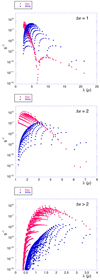	Fig. 1. Electric quadupole A_qu (red) and magnetic dipole A_ma (blue) contributions to the transition probabilities in s⁻¹ for the Q branches of the H₂ rovibrational spectrum within the ground state for Δv = 1, Δv = 2, Δv > 2.
Open with DEXTER

3. Results and discussion

The informations concerning all possible transitions within the ground electronic state of H₂ (4711) are given in electronic format. Table 2 provides the first rows of the datafile. In addition to the quantum numbers involved in the transitions, we display the transition wavenumbers σ in cm⁻¹ and their theoretical estimated accuracy (see Sect. 2.1), the wavelengths in micron and the resulting accuracy, the electric quadrupole transition probability A_qu, the magnetic dipole transition probability A_ma, the sum A = A_qu + A_ma giving the transition probability of the transition, the inverse of the total radiative lifetime τ of the upper energy level of the transition A_tot = ∑_lA_u → l in s⁻¹. We then report the energy terms of the upper level where the origin 0 is taken for the infinite separation of the two hydrogen atoms and the estimated accuracy in the same units. The next column gives the energy of the upper level expressed in Kelvin, when measured from the ground rovibrational state, as this value is used by astrophysicists when analysing the observed emission spectrum in order to derive excitation temperature, and the last column stands for the statistical weight of the upper level of the transition. We recall that the statistical weight of a particular level is given by (2J + 1)×g_I where g_I = 1 for even values of J (para levels) and g_I = 3 for odd values of J (ortho levels).

A first comment concerns the wavelengths of the actual transitions taking place within the ground electronic state of H₂. As an example, Pike et al. (2016) report the (2-1) S(27) transition of H₂ at 2.1790 μ detection towards Herbig-Haro 7. The wavelength is computed from the predictions given in Dabrowski (1984). Former (Komasa et al. 2011) and present calculations show that the energy of the v = 2, J = 29 level is not bound so that the transition is misidentified. Our present computations report a closebye transition at 2.1784 μ corresponding to (8-5) S(14) with a very low emission probability of 2.52 × 10⁻¹¹ s⁻¹, which appears not realistic. The H₂ quadrupole transition wavenumbers and corresponding emission probabilities are also displayed in the HITRAN database (Gordon et al. 2017). We have checked the overall agreement between our computations and those displayed in the HITRAN database. The transition wavenumbers values are restricted to four decimal digits in HITRAN whereas the quoted uncertainty reported in the present work is variable and spans an interval between a few 10⁻³ and a few 10⁻⁶ cm⁻¹, so that some differences in the last digits can be obtained. The number of transitions reported in HITRAN2016 is not fully complete as a result of possible numerical difficulties linked to spline interpolations of the transition moments such as those arising for CO overtone transitions, as discussed in Medvedev et al. (2016). The accuracy of our potential function and electric quadrupole as well as magnetic dipole moments prevents the occurrence of such difficulties.

A second comment concerns the relevance of the magnetic dipole contribution in the Q transitions of H₂ which has been overlooked so far in astrophysical and plasma studies. In order to quantify their possible impact we have plotted both electric quadrupole A_qu and magnetic dipole A_ma for all Q transitions by separating Δv = 1, Δv = 2, and Δv > 2 transitions. The largest contribution of the magnetic dipole compared to electric quadrupole transition probabilities is obtained for Δv = 1 transitions and λ above 3.5 μ, which involve high J rotational quantum numbers. This trend was already pointed out for the v = 1 → 0 fundamental band Q transitions by Pachucki & Komasa (2011). The differences can reach more than one order of magnitude. The available spectroscopy measurements of line strengths from Bragg et al. (1982) were restricted to low J values (J = 1, 2, 3 of the 1-0 band) and are insensitive to the magnetic dipole contribution. However, the state of the art techniques of intensity determination could allow to further check our derivations. In particular, the Q(6)−Q(10) transitions of the fundamental band show already a 6–20% magnetic dipole contribution to the radiative transition probability, which could be challenged through experiments. Finally, we think that the present computations provide the most accurate H₂ transition wavenumbers, wavelengths, emission probabilities which should be used in the analysis of high temperature plasma and astrophysical conditions.

¹

The v′=14, J′=4 level is considered as the highest bound level.

Acknowledgments

We thank the referee for his(her) pertinent suggestions which helped to improve the paper. Part of this work was supported by the Programme National de Physique et Chimie du Milieu Interstellaire (PCMI) of CNRS/INSU with INC/INP co-funded by CEA and CNES. The computational part of this work was supported by NCN (Poland) grant 2017/25/B/ST4/01024 as well as by a computing grant from the Poznan Supercomputing and Networking Center.

References

Bragg, S. L., Brault, J. W., & Smith, W. H. 1982, ApJ, 263, 999 [NASA ADS] [CrossRef] [Google Scholar]
Campargue, A., Kassi, S., Pachucki, K., & Komasa, J. 2012, Phys. Chem. Chem. Phys., 14, 802 [CrossRef] [Google Scholar]
Caswell, W. E., & Lepage, G. P. 1986, Phys. Lett. B, 167, 437 [NASA ADS] [CrossRef] [Google Scholar]
Czachorowski, P., Puchalski, M., Komasa, J., & Pachucki, K. 2018, Phys. Rev. A, 98, 052506 [NASA ADS] [CrossRef] [Google Scholar]
Dabrowski, I. 1984, Can. J. Phys., 62, 1639 [NASA ADS] [CrossRef] [Google Scholar]
Geballe, T. R., Burton, M. G., & Pike, R. E. 2017, ApJ, 837, 83 [NASA ADS] [CrossRef] [Google Scholar]
Gordon, I. E., Rothman, L. S., Hill, C., et al. 2017, J. Quant. Spectrosc. Radiat. Transf., 203, 3 [NASA ADS] [CrossRef] [Google Scholar]
Jennings, D. E., & Brault, J. W. 1983, J. Mol. Spectrosc., 102, 265 [NASA ADS] [CrossRef] [Google Scholar]
Johnson, B. R. 1977, J. Chem. Phys., 67, 4086 [NASA ADS] [CrossRef] [Google Scholar]
Kaplan, K. F., Dinerstein, H. L., Oh, H., et al. 2017, ApJ, 838, 152 [NASA ADS] [CrossRef] [Google Scholar]
Kołos, W., & Wolniewicz, L. 1964, J. Chem. Phys., 41, 3674 [NASA ADS] [CrossRef] [Google Scholar]
Komasa, J., Piszczatowski, K., Lach, G., et al. 2011, J. Chem. Theory Comput., 7, 3105 [NASA ADS] [CrossRef] [Google Scholar]
Komasa, J., Puchalski, M., Czachorowski, P., Lach, G., & Pachucki, K. 2019, Phys. Rev. A, in press [Google Scholar]
Le, H. A. N., Pak, S., Kaplan, K., et al. 2017, ApJ, 841, 13 [NASA ADS] [CrossRef] [Google Scholar]
Medvedev, E. S., Meshkov, V. V., Stolyarov, A. V., Ushakov, V. G., & Gordon, I. E. 2016, J. Mol. Spectrosc., 330, 36 [NASA ADS] [CrossRef] [Google Scholar]
Oh, H., Pyo, T.-S., Kaplan, K., et al. 2016, ApJ, 833, 275 [NASA ADS] [CrossRef] [Google Scholar]
Pachucki, K. 2005, Phys. Rev. A, 71, 012503 [NASA ADS] [CrossRef] [Google Scholar]
Pachucki, K. 2010, Phys. Rev. A, 82, 032509 [NASA ADS] [CrossRef] [Google Scholar]
Pachucki, K., & Komasa, J. 2008, J. Chem. Phys., 129, 034102 [NASA ADS] [CrossRef] [Google Scholar]
Pachucki, K., & Komasa, J. 2009, J. Chem. Phys., 130, 164113 [NASA ADS] [CrossRef] [PubMed] [Google Scholar]
Pachucki, K., & Komasa, J. 2011, Phys. Rev. A, 83, 032501 [NASA ADS] [CrossRef] [Google Scholar]
Pachucki, K., & Komasa, J. 2014, J. Chem. Phys., 141, 224103 [NASA ADS] [CrossRef] [Google Scholar]
Pachucki, K., & Komasa, J. 2015, J. Chem. Phys., 143, 034111 [NASA ADS] [CrossRef] [Google Scholar]
Pachucki, K., & Komasa, J. 2018, Phys. Chem. Chem. Phys., 20, 247 [CrossRef] [Google Scholar]
Pike, R. E., Geballe, T. R., Burton, M. G., & Chrysostomou, A. 2016, ApJ, 822, 82 [NASA ADS] [CrossRef] [Google Scholar]
Piszczatowski, K., Lach, G., Przybytek, M., et al. 2009, J. Chem. Theory Comput., 5, 3039 [CrossRef] [Google Scholar]
Puchalski, M., Komasa, J., Czachorowski, P., & Pachucki, K. 2016, Phys. Rev. Lett., 117, 263002 [NASA ADS] [CrossRef] [Google Scholar]
Puchalski, M., Komasa, J., & Pachucki, K. 2017, Phys. Rev. A, 95, 052506 [NASA ADS] [CrossRef] [Google Scholar]
Sobelman, I. I. 2006, Theory of Atomic Spectra (Alpha Science International Ltd) [Google Scholar]
Turner, J., Kirby-Docken, K., & Dalgarno, A. 1977, ApJS, 35, 281 [NASA ADS] [CrossRef] [Google Scholar]
Wolniewicz, L., Simbotin, I., & Dalgarno, A. 1998, ApJS, 115, 293 [NASA ADS] [CrossRef] [Google Scholar]

All Tables