| Issue |
A&A
Volume 630, October 2019
|
|
|---|---|---|
| Article Number | A150 | |
| Number of page(s) | 17 | |
| Section | Interstellar and circumstellar matter | |
| DOI | https://doi.org/10.1051/0004-6361/201936162 | |
| Published online | 10 October 2019 | |
Properties of central stars of planetary nebulae with distances in Gaia DR2★
1
Department of Computer Science and Information Technology, Universidade da Coruña (UDC),
Campus Elviña sn,
15071 A Coruña,
Spain
e-mail: This email address is being protected from spambots. You need JavaScript enabled to view it.
2
CITIC, Centre for Information and Communications Technology Research, Universidade da Coruña,
Campus de Elviña sn,
15071 A Coruña,
Spain
3
Department of Nautical Sciences and Marine Engineering, Universidade da Coruña (UDC),
Paseo de Ronda 51,
15011
A Coruña,
Spain
e-mail: This email address is being protected from spambots. You need JavaScript enabled to view it.
4
Instituto de Astrofísica de Canarias,
38200 La Laguna,
Tenerife,
Spain
5
Astrophysics Department; CSIC, Universidad de La Laguna (ULL), 38206 La Laguna,
Tenerife,
Spain
6
Applied Physics Department, Universidade de Vigo (UVIGO),
Campus Lagoas-Marcosende s/n,
36310 Vigo,
Spain
Received:
24
June
2019
Accepted:
24
August
2019
Abstract
Context. We have compiled a catalogue of central stars of planetary nebulae (CSPN) with reliable distances and positions obtained from Gaia Data Release 2 (DR2) astrometry. Distances derived from parallaxes allow us to analyse the galactic distribution and estimate other parameters such as sizes, kinematical ages, bolometric magnitudes, and luminosities.
Aims. Our objective is to analyse the information regarding distances together with other available literature data about photometric properties, nebular kinematics, and stellar effective temperatures to throw new light on this rapid and rather unknown evolutionary phase. We seek to understand how Gaia distances compare with other indirect methods commonly used and, in particular, with those derived from non-local thermodynamic equilibrium (non-LTE) models; how many planetary nebulae (PNe) populate the Galaxy; and how are they spatially distributed. We also aim to comprehend their intrinsic luminosities, range of physical sizes of the nebulae; how to derive the values for their kinematical ages; and whether those ages are compatible with those derived from evolutionary models.
Methods. We considered all PNe listed in catalogues from different authors and in Hong Kong/AAO/Strasbourg/Hα (HASH) database. By X-matching their positions with Gaia DR2 astrometry we were able to identify 1571 objects in Gaia second archive, for which we assumed distances calculated upon a Bayesian statistical approach. From those objects, we selected a sample of PNe with good quality parallax measurements and distance derivations, we which refer to as our Golden Astrometry PNe sample (GAPN), and obtained literature values of their apparent sizes, radial and expansion velocities, visual magnitudes, interstellar reddening, and effective temperatures.
Results. We found that the distances derived from DR2 parallaxes compare well with previous astrometric derivations of the United States Naval Observatory and Hubble Space Telescope, but that distances inferred from non-LTE model fitting are overestimated and need to be carefully reviewed. From literature apparent sizes, we calculated the physical radii for a subsample of nebulae that we used to derive the so-called kinematical ages, taking into account literature expansion velocities. Luminosities calculated with DR2 distances were combined with literature central stars Teff values in a Hertzsprung–Russell (HR) diagram to infer information on the evolutionary status of the nebulae. We compared their positions with updated evolutionary tracks finding a rather consistent picture. Stars with the smallest associated nebular radii are located in the flat luminosity region of the HR diagram, while those with the largest radii correspond to objects in a later stage, getting dimmer on their way to become a white dwarf. Finally, we commented on the completeness of our catalogue and calculated an approximate value for the total number of PNe in the Galaxy.
Key words: planetary nebulae: general / Hertzsprung–Russell and C–M diagrams / Galaxy: stellar content / parallaxes / methods: data analysis
Full Table A.1 is only available at the CDS via anonymous ftp to cdsarc.u-strasbg.fr (130.79.128.5) or via http://cdsarc.u-strasbg.fr/viz-bin/cat/J/A+A/630/A150
© ESO 2019
1 Introduction
The planetary nebulae (PNe) phase represents a very short stage in the late evolution of low- and intermediate-mass stars, which occurs while they ionise their envelope to finally enter the white dwarf (WD) cooling track. This stellar evolutionary phase is interesting for a number of reasons. One reason is that PNe significantly contribute to the chemical enrichment of the interstellar medium by the ejection of processed material in the form of gas and dust. Chemical abundances can be easily derived from PNe spectra to constrain the initial composition of the progenitor star and to provide clues to mixing and nucleosynthesis processes. Emission line spectra of PNe can be used to easily identify them and their luminosity function has been used as an extragalactic distance indicator. Still, there are some fundamental open issues. In particular, the discrepancy in the distances to the central stars derived by different methods, such as parallaxes, hydrodynamical wind models, or evolutionary models using non-LTE atmospheres. This problem can only be addressed by measuring precise and consistent distances to PNe. Distances can be used to determine intrinsic properties of the nebulae, such as radii andluminosities, and allow the derivation of masses and evolutionary ages by means of evolutionary models.
Gaia satellite Data Release 2 (DR2) contains information on astrometry (parallaxes and proper motions), brightness in three bands, and radial velocities for a limited subsample of red stars for more than a billion galactic sources. These positional and kinematical measurements provide important tools to analyse the composition and evolution of the Milky Way, and they have allowed, for instance, the first complete and accurate census of the Galaxy through a Hetzsprung–Russell (HR) diagram (Gaia Collaboration 2018a), and the kinematical mapping of the different populations of stars revealing orbits, substructures, and velocity dispersions totally unexpected for an axisymmetric Galaxy in dynamical equilibrium (Gaia Collaboration 2018b). Gaia will be scanning the sky for at least four more years, while improving the quality of the obtained astrometric and photometric measurements. In the meantime, DR2 parallaxes allow the computation of distances and the derivation of the absolute luminosities of the central stars of PNe (CSPN) and the radii of the nebulae. In this paper we review some properties of the population of PNe in our Galaxy as seen through the eyes of Gaia in DR2.
Section 2 discusses the errors in the measurement of parallaxes present in DR2, the systematic corrections (zero point), statistical errors, and the way they can be used to derive statistically consistent distances (Lindegren et al. 2018; Bailer-Jones et al. 2018). In Sect. 3 we explain how we retrieved the astrometric measurements for available PNe in DR2. From all PNe identified in DR2 with available distances in Bailer-Jones et al. (2018), some statistical properties are presented. In order to study the intrinsic properties of those nebulae with reliable distance derivations, we selected a sample of PNe, which we call the Golden Astrometry PNe (GAPN), with good quality parallax measurements and distance derivations, by imposing quality cuts in the available measurements of parallaxes. Some additional cleaning was carried out to exclude objects from this sample that were misclassified as PNe or post-AGB stars.
In Sect. 4, galactic distribution and distances adopted for GAPN are presented and compared with those obtained with previous determinations of distances using astrometry (Harris et al. 2007), non-local thermodynamic equilibrium (non-LTE) models (Napiwotzki 2001), and other methods (Stanghellini & Haywood 2010; Frew et al. 2016; Schönberner et al. 2018). Using these distances, nebular radii are also estimated, derived from angular sizes in the Hong Kong/AAO/Strasbourg/Hα (HASH) database (Parker et al. 2016). Nebular absolute sizes and literature expansion velocities (with a correction) for a suited subsample of nebulae are used to derive kinematical ages, as shown in Sect. 5.
Section 6 is devoted to analysing the physical properties of some of our GAPN based on their distances and on literature values of their visual magnitudes, interstellar reddening, and effective temperatures. We calculate the luminosities and derive the star temperature versus luminosity positions in the HR diagram, which can be discussed in comparison with updated evolutionary tracks in Miller Bertolami (2017). Finally, an estimation of PNe density, scale height, birth rate, and total number of nebulae in the Galaxy are provided in Sect. 7, using a procedure based on Frew (2008) and compared with other literature results such as Zijlstra & Pottasch (1991) and Pottasch (1996). We also analyse the completeness of our general sample and, finally, summarise our conclusions.
2 Parallaxes and distances in DR2
In Gaia DR2, parallaxes and their uncertainties are given with a great accuracy, milliarcseconds (mas), but the formal uncertainties listed in DR2 are estimated from the internal consistency of measurements and they do not represent the total errors. Following Lindegren et al. (2018), the total error in DR2 parallaxes is the addition of random (internal) and systematic errors, the latter including the parallax zero point, and they are dependent, at least, on position, magnitude, and colour. This is in part due to patterns imprinted by the Gaia scanning law and to the spacecraft attitude errors.
On the one hand, parallaxes need a bias correction called “zero point”, w0, and according to the study of Lindegren, as a global average, this parameter takes a value of −0.03 mas. On the other hand, it is necessary to correct the internal error of parallax measurements, σi, where values depend on the specific source as given by Gaia DR2. Additionally, DR2 parallax measurements are subject to systematic errors, σs, which depend on the brightness of the object (i.e. G magnitude in the Gaia photometric system). The total error, σT, can be obtained from

where k is estimated to be 1.08 (Lindegren et al. 2018). Following DR2 documentation, we calculated the total error as follows:
![Mathematical equation: \begin{equation*}\sigma_{\textrm{T}} = \left\{\!\!\! \begin{array}{ll} \sqrt{1.08^{2}\times\sigma_{\textrm{i}}^{2}+(0.043)^{2}}, & \mathrm{if\ } G > 13 \\[6pt] \sqrt{1.08^{2}\times\,\sigma_{\textrm{i}}^{2}+(0.021)^{2}}, & \mathrm{if\ } G \leq 13 \end{array} \right.\!\!\! .\end{equation*}](/articles/aa/full_html/2019/10/aa36162-19/aa36162-19-eq2.png) (1)
(1)
Once computed, total uncertainties in parallaxes can be used to establish confidence criteria in our selection of stars, which allows us to work with reliable distance values derived from them. Additionally, we considered the recommended goodness-of-fit indices for Gaia DR2 astrometry (Lindegren et al. 2018), the unit weight error (UWE), which is computed from the astrometric chi square test of the measurements, and the renormalised unit weight error (RUWE), which uses an empirical normalisation factor provided in DR2 ESA web page. We chose the limiting values of both quantities that are recommended in DR2 documentation, i.e. UWE < 1.96 or RUWE < 1.40.
The derivation of distances from parallaxes (πtrue) with high uncertainties is not straightforward because distance “r” has a non-linear relationship to the measured quantity, r = 1∕πtrue, and it is constrained to be positive (Luri et al. 2018). A useful approach is to consider some assumptions about the distribution of the distances in our Galaxy, known as a prior within a statistical Bayesian analysis. As discussed in Bailer-Jones (2015) and Astraatmadja & Bailer-Jones (2016), a possibility is to assume that the a priori probability volume density of stars in the Milky Way is exponentially declining with some appropriate distance scale. This exponentially decreasing space density (EDSD) is explicitly endorsed in DR2. We decided to use the Bailer-Jones et al. (2018) catalogue of estimated distances from DR2 parallaxes, which uses an EDSD with a distance scale L that varies as a function of galactic latitude and longitude, according to a model suited for Gaia observations. In the next sections we discuss the distance errors and the distribution of distances obtained for our sample of PNe.
3 Selection of a sample of PNe central stars with distances and reliable distances in DR2
3.1 General selection
There are several compilations of PNe and CSPN in recent literature, among which we chose the following: Kerber et al. (2003); Stanghellini & Haywood (2010); Weidmann & Gamen (2011); and HASH database (Parker et al. 2016). Firstly, we considered the objects contained in the first three catalogues (Kerber, Stanghellini, and Weidmann), taking into account both coordinates and names. Next, we complemented our compilation selecting the objects catalogued as “true PN” in the HASH database, which includes, in addition to the other catalogues, new objects that were detected in several Hα surveys.
Thus, intotal, we ended up with 2554 sources. The next step was to verify which of these objects were observed by Gaia in DR2. It is understood that Gaia observations are aimed to detect unresolved sources, in our case PNe central stars; hence, PNe without a visible central star or with a very faint star are not expected to be catalogued in DR2. For this task we used the ARI’s Gaia Services andwe did queries by list to the Gaiadr2.gai_source table using the coordinates or the names of the PNes. By obtaining the closest Gaia object for each coordinate/name given in our PNe list, we retrieved Gaia DR2 measurements (parallaxes, G magnitudes…) when available, reaching a number of 1948 sources with measured parallaxes. Among these, we further checked for objects with dubious identifications, keeping only those objects with coordinates not farther than 5 arcsec from those listed in DR2, finding a total number of 1736 objects.
This list of objects was then queried to the Simbad database, doing an X-match with Gaia’s objects coordinates to obtain more parameters of the sources (object type, photometry, angular size, radial velocity …) provided by this database. Several sources in our catalogue were identified by Simbad with an object type other than “PN” and were excluded from our list. So, we ended up with a final list of 1571 objects.
Once the Gaia DR2 ID of the objects were obtained, we proceeded to retrieve their estimated distances from us by querying the gaiadr2_complements.geometric_distance table in DR2. This table lists the values of the estimated distances, using the Bayesian approach by Bailer-Jones et al. (2018) mentioned in the previous section. Apart from the estimated distances, this approach provides lower and upper bounds of the distance values, among other parameters.
The distributions of parallaxes relative errors and distance errors (higher and lower bounds) are shown in Fig. 1 More than 600 PNe have their parallaxes measured with relative errors higher than 100%, which translates into errors in the derivation ofdistances higher than 50% for most of the stars in our sample (for the upper bound of errors). Meanwhile, Fig. 2 shows the histogram of the derived distances, for the sample of 1571 PNe with distances in DR2.
We are aware of the problem that the use of parallaxes with large uncertainties translates into distances and other astrophysical quantities derived from them, such as luminosities and sizes. As discussed in Luri et al. (2018), truncation of data using a threshold for the parallax relative error, or the exclusion of objects with negative measured parallaxes from a sample, makes the distribution of distances unrepresentative and can lead to wrong conclusions regarding the statistical properties of the sample. Consequently, we decided to keep the complete sample for the discussion regarding general properties of our sample, such as the distance distribution of PNe and the estimation of the number of PNe in our galaxy. Conclusions in such cases can only be formulated among the appropriate errors reported for the measured quantities.
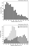 |
Fig. 1 Parallax relative errors (upper) and low and high distances relative errors (lower). |
 |
Fig. 2 Distances to PNe in DR2 derived with a Bayesian approach (Bailer-Jones et al. 2018). |
3.2 Selection of sample with reliable distances
A different approach can be followed if we intend to derive individual properties for a subsample with high quality measurements of both parallaxes and the corresponding distances. With this objective in mind, we constructed a sample of PNe with reliable distances in DR2, our GAPN, with constraints in the following properties:
Angular distance: the distance in arc seconds between the PN coordinates and the closest object detected by Gaia. We chose objects with angular distances lower than 5 arcsec from the original coordinates.
Parallax relative error: obtained by taking into account all reported internal and systematic errors, as explained in Sect. 2. We chose a threshold for parallax relative errors of 30%.
Low/high distance relative error: obtained by taking into account both low and high bounds in distance, given by the adopted Bayesian approach. We selected objects with relative errors for both lower and upper distance bounds lower than 30%.
Unit weight error (UWE): this is defined as
 , where χ2 is the astrometric_chi2_al value and N is the astrometric_n_good_obs_al value. These parameters are provided by Gaia database. We set a lower threshold value for UWE of 1.96, following the recommendation in Lindegren et al. (2018).
Renormalised unit weight error (RUWE): this is the UWE value divided by the normalisation function U0 (G, C) (or U0 (G) for sources without known colour). This function depends on the brightness and colour of the sources, G (“phot_g_mean_mag”) and on C = GBP − GRP and has been interpolated from the tables provided in (“ESA Gaia DR2 known issues” page). The RUWE lower threshold value was set to 1.4 (Lindegren et al. 2018).
In order to check the identification of some dubious sources, we studied in detail those located farther than 2 arcsec from DR2 coordinates, those objects with distances beyond 8 kpc from us, and those whose nebular radius was estimated as larger than 1 pc (using bibliographic angular sizes and the obtained distances, as we explain later in the paper). So, finally, after discarding all dubious cases, we ended up with a catalogue of 211 GAPN.
4 Discussion on galactic distribution, distances, physical sizes, and radial velocities
As shown in Fig. 2, the distribution of distances for the sample of 1571 PNe is rather smooth. This distribution can be fitted with a Gaussian function with maximum value at 3.55 kpc and sigma 1.94 kpc. To visualise how errors are affecting distance derivations, in Fig. 3 we show the number of PNe at several distance intervals (0–500 pc, 500–1000 pc, 1000–1500 pc, and 1500–2000 pc); relative errors are binned at 10 or 20% intervals. This is plotted for both distance error bounds, i.e. low and high. It can be seen that while in the case of the lower bound errors values higher than 50% are found for a very marginal number of PNe, if higher bounds of errors are considered the behaviour is very different; a significant number of nebulae beyond the first 500 pc are affected by relative errors of the order of 50% and higher. In the following sections we focus on the selected sample of 211 PNe with very reliable distances, the GAPN sample.
4.1 Galactic distribution, parallaxes, and distances for GAPN
Figure 4 shows the spatial distribution in galactic coordinates for GAPN planetaries. As expected, most of the PNe are located close to the galactic plane, and about 60% of the objects are located at latitudes between 10 and −10 degrees. It can also be appreciated that there are more PNe closer to the galactic centre, with more than 25% of GAPN located at galactic longitudes between −30 and 30 degrees. The exact coordinates and Gaia DR2 ID’s of this sample objects can be seen in Table A.1.
Figure 5 shows the distribution of parallax relative errors for our catalogue of GAPN, which are always below 30% owing to our selection criteria. If we study the relationship between the parallax relative error and the brightness of the star, we do not find a simple trend; but we can conclude that for stars brighter than G = 10, parallax relative errors are below 5%, while for those stars with G values between 10 and 12, parallaxes tend to be bounded below 15%.
The upper panel of Fig. 6 presents the distribution of nebulae as a function of distance inferred for our GAPN. From a distance close to 2 kpc, the number of nebulae decreases. To analyse if this can be related to the completeness of our sample, we plotted the distribution of sources in the galactic centre direction in the lower panel of Fig. 6, where the galactic longitudes are −90° < l < 90°; there are a total of 137 nebulae.
Both distributions are similar, showing a decrease of the number of sources at distances beyond 2 kpc. From this we can infer that our selection of sources with good astrometric measurements is probably limited in completeness, approximately to such a distance. We return to the completeness of our sample in Sect. 7.4. In Table A.1 all numerical values about parallaxes and distances are shown together with their uncertainties.
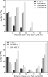 |
Fig. 3 Relative errors in distances for different distance ranges derived from DR2 parallaxes upon a Bayesian approach (Bailer-Jones et al. 2018). Errors are shown for lower (upper panel) and higher (lower panel) bounds. |
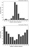 |
Fig. 4 Distribution of PNe in galactic coordinates: latitude (upper panel) and longitude (lower panel). |
 |
Fig. 5 Distribution of parallaxes relative errors for PNe in the GAPN subsample. |
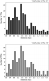 |
Fig. 6 Histogram of distances for GAPN: for the full sample (upper panel) and only for objects in the galactic centre direction with longitudes between −90° and +90° (lower panel). |
4.2 Comparison with other distance determinations
We can compare our DR2 distances with other literature values obtained from astrometric measurements or from other (indirect) methods. In particular, we compared our estimations with those of Harris et al. (2007), for astrometry; Napiwotzki (2001), for non-LTE model stellar atmosphere fitting; Stanghellini & Haywood (2010), for statistical distances; Frew et al. (2016); for surface brightness versus radius; and Schönberner et al. (2018), for hydrodynamical model fitting. This comparison is illustrated in the various panels of Fig. 7, where the dotted line is the 1:1 relation and the solid line represents the linear regression between the two determinations, which help us to visualise how far the results are from each other. All the points are represented within their error bars.
A comparison with other astrometric distances, such as those in Harris et al. (2007), shows a good agreement between uncertainties (upper panel of Fig. 7). A similar result was found in Kimeswenger & Barría (2018) synoptic study of PNe distances in DR2. Statistical distances (Stanghellini & Haywood 2010) do not agree with Gaia distances, showing overestimated values in many cases. A linear fit to these distances leads to a bias of 1 kpc. However, panel c in Fig. 7 shows that such bias is affected by the presence of a marginal group of objects displaying wide discrepancies with DR2. A possible explanation is that those objects are bipolar or butterfly-like PNe, and such a statistical method cannot be applied to those classes of nebulae.
We now comment on non-LTE model stellar atmosphere fitting to derive distances. From the pioneering work of Mendez et al. (1988), followed by Kudritzki et al. (2006), and Pauldrach et al. (2004), several authors have used non-LTE model stellar atmospheres to derive distances. The analysis of the stellar spectra delivers Teff and surface gravity g values, which are then used to estimate themass from a Teff vs. log (g) diagram with calculated post-AGB evolutionary tracks. So far, this method has been applied to 27 CSPN (Napiwotzki 2001). We find that Napiwotzki (2001) distances tend to be larger than DR2 distances (see panel b in Fig. 7). A linear fit provides a bias around 400 pc with respect to Gaia distances. In view of these results we think that it is worthwhile to review current non-LTE model stellar atmospheres, applied to very hot CSPN, as described below.
It is interesting to note that Napiwotzki (2001) discussed the existence of positive bias between his spectroscopic distances and those obtained from United States Naval Observatory (USNO) and Hubble Space Telescope (HST) parallaxes and concluded that sample truncation in distance or in parallax values can explain such discrepancies between statistical uncertainties of the order of 20%. His simulations imply that astrometric distances should be corrected for an undetermined quantity due to a positive bias. Positive bias is a well-known effect that appears when sample truncation is done based, for instance, on the quality of the parallaxes. Our GAPN sample distances were derived using a Bayesian procedure that allows very small or negative parallaxes to have their corresponding distances calculated between confidence intervals. Once distances were derived, we selected useful values by, among others, constraining the goodness of fit indices of Gaia astrometric measurements. Even considering some possible positive selection effect in the distances derived for our GAPN sample, astrometric distances would be overestimated and not underestimated as they are in this case.
We would like to point out that the discrepancies between astrometric and spectroscopic non-LTE distances that we are discussing are evident only for central stars (CS) with Teff larger than 90 000 K. In Fig. 7b there is a small sample of CS with distances in Napiwotzki (2001) (star symbols) that are compatible with DR2 derivations, and they all fall in this low Teff regime. A plausible explanation has been indicated by D. Lennon (priv. comm.) in the sense that non-LTE models are not using line-blanketing for metals.
Finally, when considering the case of Frew et al. (2016) and Schönberner et al. (2018) determinations, we found no clear bias between their results and our derivations (see panels d and e of Fig. 7). The Frew et al. (2016) distance scale was based on a statistically derived relation of the Hα surface brightness evolution with nebular radius. Schönberner et al. (2018) calculated the distances to 15 round-shaped PNe by measuring the expansion velocity of the nebular rim and shell edges, and by correcting the velocities of the respective shock fronts with 1D radiation-hydrodynamics simulations of nebular evolution. The latter authors found a reasonable agreement with literature values except with those obtained with non-LTE model atmosphere fitting (spectroscopic gravity distance). They explained such differences as due to the fact that CSPN mass is not a measured quantity. The mass value depends on the chosen post-AGB evolutionary track and, for instance, the inclusion of overshooting leads to lower masses for a given luminosity. Evolutionary tracks in the literature do not include overshooting. Interestingly, Schönberner et al. (2018) discussed the use of updated evolutionary models for the calculation of luminosities and masses and concluded that spectroscopic gravity distances are, in general, higher than those derived by other methods and can produce unreasonably high luminosities. This conflicts with the predictions from stellar evolutionary theory because central star masses are even beyond the Chandrasekhar mass limit in some cases.
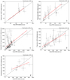 |
Fig. 7 Comparison between DR2 and other distance derivations. |
4.3 Physical radii
The knowledge of distances allowed us to obtain the physical size of the PNe from the observed nebular angular sizes. The HASH database lists major and minor axis angular diameters for most of known PNe derived from Hα photometry. A typical radius for the nebulae (R) can then beobtained without taking into account the projection effects or the complexity of some of the nebular shapes, simply by considering the average angular radius in arc seconds from the Hα 10% isophote and DR2 distances.
Figure 8 shows the distribution of such typical radii for the case of low latitude nebulae, with latitude values between 10 and −10 degrees, as compared with the remaining objects. Without going into the details about the morphology of the nebulae, which is beyond the scope of this work, it can be noted that 70% of the PNe radii are larger than the typical PNe value of 0.1 pc (Osterbrock & Ferland 2006). We found that PNe close to the galactic plane represent a wide range of sizes and do not show any trend to be larger, as would be expected if they mostly evolved from high-mass progenitors with higher expansion velocities (Corradi & Schwarz 1995). Table A.1 lists the typical radius for 206 GAPN present in the HASH database.
 |
Fig. 8 Planetary nebulae physical radii for objects near the galactic plane (− 10° < lat < 10°) and for the rest of galactic latitudes. |
4.4 Radial velocities
It is also interesting to analyse the radial velocities of our GAPN sample and to compare their values with those expected for a pure circular galactic rotation. We retrieved radial velocities from the literature for a total of 125 PNe (see Table A.1). The upper panel of Fig. 9 shows the distribution of systemic radial velocities corrected to the local standard of rest (LSR). The lower panel of the figure indicates the radial velocities as a function of the galactic longitude. Filled circles correspond to objects located near the galactic plane (latitudes lower than ±10°). We found that, in general, our low latitude GAPN sample follows grosso modo the radial velocities sinusoidal curves expected for their range of distances, considering the case of pure circular rotation for a flat rotation disc at 230 km s−1. Some nebulae display a wide velocity departure from pure rotation. These are mostly nebulae with galactic longitudes close to zero, i.e. those in the direction of the galactic centre, which are expected to show a high velocity dispersion and a departure from the rotational general trend. A detailed study is also beyond the scope of this work.
5 Radii, expansion velocities, and kinematical ages
The fact of having, for the first time, precise parallaxes that allow us a consistent estimation of distances and physical sizes of a meaningful sample of nebulae, offers us the opportunity to calculate their ages based on nebular sizes and expansion velocities. We also briefly discuss the limitations and hypothesis under which these determinations have been carried out in the literature.
It has been common practice to derive the so-called kinematical ages as the ratio of the nebular size and expansion velocity, this latter calculated from the broadness or splitting of the most brilliant nebular lines, mainly from [OIII], [NII], and Hα. As has been reviewed by several authors (Schönberner et al. (2014) and references therein), the velocity field of a PN is a complex structure that depends on the CS mass; this velocity field does not vary not linearly with time, apart from other considerations regarding, for instance, the density structure of the nebulae. Furthermore, precise values of expansion velocities also depend on the excitation level of the emission lines used to derive them (the so-called Wilson effect). Usually, expansion velocities are measured inthe inner bright rim of the nebular structure, while nebular sizes refer to the outer shell of the objects. There are both observational and theoretical evidences that velocities in the shell and in the rim are different during most of the evolution of the nebulae (Villaver et al. 2002; Corradi et al. 2007; Jacob et al. 2013). The post-shock velocity, i.e. the flow velocity immediately behind the leading shock of the shell (or the outer edge of the shell), has also been proposed as a simplerproxy of the true nebular expansion speed (Schönberner et al. 2005; Corradi et al. 2007; Jacob et al. 2013), but this value is only available in the literature for a small sample of nebulae because it is difficult to measure.
Villaver et al. (2002) simulations of the dynamical evolution of the circumstellar gas around PNe demonstrated, for the first time, that nebular shells are subject to acceleration during their evolution and that the kinematical ages, as derived from sizes and expansion velocities, can significantly depart from the CS evolutionary time. These authors found that the kinematical ages are always higher than the CS ages when the nebula is younger than 5000 yr while, for intermediate ages (between 5000 and 10 000 yr), the ages derived from a dynamical analysis tend to overestimate the age of the CS for high-mass progenitors (in their simulations, 3.5 and 5 M⊙) and to underestimate it for the low-mass progenitors.
Schönberner et al. (2005), using 1D hydrodynamic simulations of nebulae envelopes, pointed out that rim and shell velocities are usually very different from each other, unless the nebula is rather old (ages greater than 8000 yr) and the star is approaching its maximum temperature. Jacob et al. (2013) showed how hydrodynamic models of the evolution of the envelopes can be used to derive correction factors for the measured expansion velocities (both for rim and post shock velocities) that can, then, be used to derive more realistic values for the true expansion speed of the outer nebular shell.
From the information above, it is evident that while the use of hydrodynamic models and their interpretation with data is being discussed, a consistent set of nebulae data is mandatory to be able to compare observations of nebulae expansion velocities and kinematical ages derived from them with other model-dependent quantities, such as evolutionary ages or the total number of PNe in a stellar population, as derived from population synthesis models.
In Tables A.2 and A.3, we show a compilation of 68 PNe with good DR2 distances (i.e. belonging to our GAPN sample) with consistent literature values for their Teff, interstellar extinction values, visible magnitudes, expansion velocities, and the corresponding kinematical ages. After examining several literature PNe data sources, we decided to use data on PNe properties in the compilation by Frew (2008). Temperatures, in particular, are taken from Frew (2008) or from Frew et al. (2016). Absolute visible magnitudes are based on the Frew (2008) reported magnitudes, corrected with DR2 distances, and expansion velocities correspond to the values also listed in Frew (2008; Table 9.4), while [NII] and post-shock velocities are from Jacob et al. (2013). Additionally, we imposed that the objects are neither known binaries nor H-deficient PNe, and that they have a nearly spherical shape (Rmin ≥ 0.8 × Rmax). Expansion velocities reported in Frew (2008) were measured as a weighted average of available literature values, and no information about the specific ion or method (line broadness or line splitting) is provided by the author. For those cases where [NII] velocities are available from Jacob et al. (2013), we were able to compare them with Frew (2008) velocities and we found a general good agreement among them (no significant bias and a mean dispersion around 5 km s−1). We also found that post-shock velocities are always higher than [NII] velocities with a positive bias of about 15 km s−1.
In view of the discussion above, it seems that a reasonable option is to correct the rim expansion velocities using the correction factors in Jacob et al. (2013) to account for the fact that the rim velocities are lower than the overall nebular expansion velocities for most of the evolutionary time. In Jacob et al. (2013), correction factors of the order of 1.3–1.6 are proposed for the different kinematical scenarios for most of the lifetime of nebulae. The exact value of the correction factor depends on the mass of the CS and on its evolutionary stage and, also, on hydrodynamical modelling. Taking into account the rather high uncertainties in the velocity data, we decided to consider an overall value of 1.5 for the correction factor for rim velocities to derive the corresponding kinematical ages. This correction value is similar to that adopted by Gesicki et al. (2014), who used the Perinotto et al. (2004) hydrodynamical models to calibrate the relation between the average expansion velocity, radius, and age.
Considering all this information, we were able to select a sample of 45 nebulae with reliable expansion velocities, whose distribution is shown in Fig. 10 (upper panel). It can be observed that most of these have expansion velocities between 30 and 50 km s−1.
In addition, we can estimate an average expansion velocity and its typical deviation, so that we obtain

This estimation is close to the value of 42 ± 10 km s−1 given by Jacob et al. (2013). Once we know the nebular expansion velocity, it is possible to estimate the so-called kinematical age for each PN by a simple relation, such as

In Fig. 10, we show the distribution of the kinematical ages that we found for our sample of PNe. Although most of the PNe are rather young, with ages under 15 000 yr, we also found nebulae spanning ages well beyond those values.
Now, we can also estimate an average value for the kinematical age of the sample, which is known as visibility time (⟨ TVT⟩) of a PNe population (Jacob et al. 2013). This can be derived from the average expansion velocity and average radius as follows:

Then, the visibility time can be calculated as

This visibility time is very similar to the value of (21 000 ± 5000) yr given by Jacob et al. (2013). We should stress the limitations of this derivation. Firstly, simply because our statistics is rather poor, and secondly, because we probably have a bias with age, with more young PNe than old because PNe tend to dim as they get older. To study such trend we analysed separately the ages of those PNe that are located closer than 1 kpc versus those located farther away. As expected, we found that the distribution of ages for the nearby sample is rather homogeneous while, for the second sample, nebulae tended to be younger.
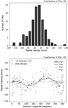 |
Fig. 9 Distribution of systemic radial velocities (upper panel) and radial velocities as a function of galactic longitude (lower panel) for a selection of objects in the GAPN sample. |
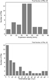 |
Fig. 10 Distribution of expansion velocities (corrected) from the literature (upper panel) and kinematical ages derived from them (lower panel). See text for details. |
6 Temperatures and luminosities of the central stars
Reliable distance determinations obtained from Gaia astrometry allow us to consider the exercise of placing these PNe in a HR diagram and to analyse if it is possible to obtain some useful information about their evolutionary status, by comparing the distribution of objects with the positions predicted by the most recent evolutionary models (Miller Bertolami 2017). Furthermore, we can compare the evolutionary ages with kinematical ages obtained in the previous section. To carry out this analysis it is necessary to compile reliable information on the central star effective temperatures (Teff) and the necessary information to calculate the luminosities of the objects. In particular, we need visible magnitudes, distances, extinctions, and bolometric corrections.
6.1 Effective temperature
Central stars Teff are often estimated with the Zanstra method (Zanstra 1928) by measuring H I and He II nebular fluxes, or at least one of them, and taking into account the value of the V magnitude of the star and the nebular extinction.
Frew (2008) listed Teff estimations based on different bibliographic sources, focussing on the values obtained from Helium Zanstra method. After examining several literature compilations with PNe data on Teff, visual magnitudes, and interstellar reddening derivations, we decided for consistency to centre our analysis on the sample of GAPN in common with the Frew (2008) compilation. We selected objects with precise values rather than bounded values. Also, we restricted our selection to those objects that are neither known binaries nor H-deficient PNe. Figure 11 presents PNe temperatures with their errors for 68 PNe in common with our GAPN sample. Most of these have Teff between 90 000 and 120 000 K and a bias towards high temperatures because the stars with Teff < 45 000 K do not produce He twice ionised (Kaler & Jacoby 1991).
 |
Fig. 11 Histogram of CSPN effective temperatures for objects in GAPN with data in Frew (2008). |
 |
Fig. 12 Absolute visible magnitude for stars in GAPN in common with Frew (2008). |
6.2 Brightness, extinction, and luminosity
We now focus on the brightness and luminosities of our sample of CSPN. Gaia G-band magnitudes, GBP −GRP colour, and V values (taken from Frew 2008) are shown in Table A.3. Most of the stars have G magnitude values between 12 and 18, a distribution that peaked at 15.5 magnitudes, and negative GBP −GRP colour values, as corresponds to their high temperatures. In addition, V values range between 10 and 20 magnitudes and peak around 16.5 magnitudes. We compared the G and V magnitudes object by object to further check for data consistency in our sample. Table A.3 also lists Frew (2008) extinction values for the sample of 68 PNe selected from our GAPN. The great majority of stars have very low extinction in the range 0–0.2 magnitudes.
Absolute visible magnitudes can then be derived taking into account our DR2 distances and extinctions from Frew (2008) (Fig. 12). These magnitudes span values between 2 and 8 for most of the stars, which is the expected range during the evolutionary stage of PNe.
Absolute bolometric magnitudes, MB, were derived using the calibration procedure published by Vacca et al. (1996), i.e.

where

These bolometric corrections were calculated for O and early B spectral types assuming a maximum Teff = 50 000 K. However, this relation depends only weakly on the surface gravity of the star, so we assumed that it is correct for higher temperatures. From bolometric magnitudes we derived the luminosities. Both quantities are shown in Figs. 13 and 14.
 |
Fig. 13 Absolute bolometric magnitude for stars in GAPN in common with Frew (2008). |
 |
Fig. 14 Luminosity for stars in GAPN in common with Frew (2008). |
6.3 Location in the HR diagram
Once the luminosities are derived, the stars can be plotted on a HR diagram to compare their distribution with the prediction of evolutionarymodels for post-AGB stars. We decided to make a comparison with the new evolution tracks by Miller Bertolami (2017) because they include updated opacity values, both for the low and high temperature regimes and for both the C- and O-rich AGBstars. These models also included conductive opacities and nuclear reaction rates that have been updated, and a consistent treatment of the stellar winds for the C- and O-rich regimes. The author explains that the new models reproduce several AGB and post-AGB observables that were not reproduced by the older grids (see Miller Bertolami 2017 for details). From these models, post-AGB timescales are approximately three to tentimes shorter than those of old post-AGB stellar evolution models, and luminosities are about 0.1− 0.3 dex brighter than from previous models with similar remnant masses.
Figure 15 shows such HR diagram together with the evolutionary tracks for a wide range of masses. Considering the location on the HR diagram of the stars, we interpolated masses and evolutionary ages, as shown in Fig. 16. Numerical values can be consulted in Table A.3. Most of the stars have masses between 0.525 and 0.625 M⊙.
For a more detailed study, we divided the HR diagram into three regions. The first region corresponds to the stars in a very early stage, while they are increasing their temperature (till log (Teff) = 4.8) at a rather constant luminosity value and fulfilling  . The second region corresponds to the same flat luminosity part of the HR diagram, but for higher temperatures, from log (Teff) = 4.8 until the maximum Teff value. Finally, the third region covers the evolution of objects that have reached their maximum temperatures as PNe and are decreasing in luminosity (
 ) on their way to becoming a WD star. We now analyse our Gaia DR2 derived quantities that, in the case of the CSPN, are updated luminosities and, for the nebulae, are the physical radii; this physical quantity increases its value with evolution as the nebulae expand. We aim to see if the new models allow us to draw a consistent picture of the evolutionary stage of the objects. We limit this analysis to a subsample of PNe with expansion velocities obtained from the literature (55 PNe out of 68 PNe, see Table A.2).
In Table 1 we present the mean values we obtained for masses, physical radii, and evolutionary ages in each of the three HR diagram regions. The masses mean values are similar in the three regions. Because evolutionary times in the early stages are very short, high-mass objects tend to pile up in the later stage. Regarding radii and evolutionary ages, as expected, there is a clear increase per region of the mean values in both parameters. We find values for the mean radius of 0.093, 0.298, and 0.804 pc, respectively. The mean values of evolutionary ages in each of the regions are 14.2, 20.5, and 33.8 kyr, respectively. Such mean ages show a high dispersion because in each of the regions there are objects with all possible mass values and evolutionary times depend strongly on mass. Following Miller Bertolami (2017), to compile such ages, we added a transition time from an early post-AGB stage until Teff = 7000 K (or log (Teff) = 3.85). Such transition times are about 1 kyr for the highest mass CSPN and 2 kyr for the remaining masses.
Secondly, considering evolutionary ages and radii, we can estimate the mean expansion velocities spanned by the nebulae and compare those values with those reported in the literature and discussed in Sect. 5. The only region where we found consistent values (in mean) is the latest evolutionary phase, when the stars are very evolved objects already cooling towards the white dwarf stage. Noticeably, expansion velocities for our sample of 31 objects in common with Frew (2008) in this region have a mean value of around 24 km s−1 (without correction factor), which coincides with the mean expansion velocity that we can derive from evolutionary ages and radii. In any case it has to be pointed out that the dispersion of the values of the last quantity is very high. In the other two regions, corresponding to an early evolutionary phase, expansion velocities mean values are very low in comparison with Frew (2008) observational velocities. It should be taken into account that evolutionary ages depend strongly on the value of Teff, and they are very different depending on the mass value adopted for the CS. Estimations of mean expansion velocities in the early evolutionary stages are subjected to a larger uncertainty than those in a more advanced stage.
It is important to stress again that, in general, we find quite a high dispersion for the mean values of radii, ages and, consequently, evolutionary expansion velocities, because we are dealing with stars with different masses, i.e. stars that evolve at significantly different velocities. Despite this, we found that the position in the HR diagram of the stars provides valuable information about the PN evolutionary state, and that the expansion and size of the envelopes agree in general terms with the evolutionary state of the CS. Mean values of all these parameters and their typical deviations are presented in Table 1. In this study, we do not discard objects according to their geometric shape to obtain their expansion velocity, and therefore we have a selection of 54 PNe (and not 45 as in Sect. 5).
It is interesting to note that three stars in Fig. 15 appear to be located out of the Miller-Bertolami evolutionary tracks, lying to the lower Teff zone. The accompanying PNe are PN We 1-10, PN K 2-2, and PN M 2-55. We searched in detail the available literature about these sources and came to the conclusion that the most plausible hypothesis about their atypical location in the HR diagram is that they are born-again PNe (Herwig et al. 1999), two of which (PN We 1-10 and PN K 2-2) are very large nebulae that have rather low expansion velocities and correspondingly, large kinematical ages. The CS Teff and luminosity values for the three of these fit well with He-burning evolutionary tracks (see for instance Iben 1984). More work, however, is needed to confirm this explanation.
 |
Fig. 15 Hertzsprung–Russell diagram for a selection of GAPN stars, together with Miller Bertolami (2017) evolutionary tracks. |
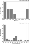 |
Fig. 16 Estimated masses and evolutionary ages derived from Miller Bertolami (2017) evolutionary tracks. |
Mean values of different parameters in three regions of the HR diagram, together with their dispersion values, in brackets.
7 Properties of PNe population in the Galaxy
The total number of PNe populating our Galaxy is an intrinsically interesting value that can be used to study the underlying population from which they derive. For instance, evolutionary times and progenitor masses can be used to constrain the SFH for the range of ages covered by the PNe. Using the information regarding 3D positions of the PNe obtained from Gaia DR2, for the complete sample of 1571 PNe, we can estimate the total population of PNe in the Milky Way.
7.1 Density
Firstly, we need to calculate the density of PNe in our neighbourhood and, as a first approximation, we can assume that such value can be extrapolated to the whole Galaxy. Following the procedure by Frew (2008), we calculated the number of stars inside a cylindrical volume around the Sun. We considered a radius of R = 2 kpc, which is close enough to claim for completeness and far enough to have a considerable number of PNe for statistical significance (see Fig. 6). We calculated the number of PNe inside a cylinder with radius r fulfilling r = D ×cos (ϕ) < 2 kpc (without height restrictions), where D is the distance and ϕ is the latitude in radians, obtaining a total of 374 PNe.
Then, we calculated the scale height Hz, i.e. the galactic height where the PNe population density decreased by a factor e from the galactic plane. We assumed that the Sun is close enough to the galactic plane. The heights from the galactic plane can be calculated as z = D ×sin (ϕ). The numerical values can be seen in Table A.1 and their distribution is shown in Fig. 17 in bins of z = 25 pc. This information can be used to derive Hz by a linear regression as shown in Fig. 18. Only PNe with |z < 600| were used for the fit because for higher altitudes the statistic is poor. We obtained the following relationship:
 |
Fig. 17 Galactic heights (absolute value) distribution for those PNe inside a cylinder with radius of 2 kpc. |
 |
Fig. 18 Logarithm of PNe population density as a function of the galactic height (absolute value), together with the linear regression. |

where an average quadratic error of σ2 = 0.34 was found. The corresponding value of the scale height is

which has an uncertainty of several tens of parsecs (see Sect. 7.4 for details). This value is lower than that provided by Frew (2008)of 217 ± 20 pc, but within the range of 180 ± 20 pc given by Pottasch (1996).
Once Hz has been derived, we can estimate the density of PNe in the Galaxy. If we consider only those PNe with an absolute galactic height below the scale height and inside a cylinder with radius 2 kpc, we obtain a total number of Nc = 269 PNe. The density can then be calculated taking into account the number of stars and the cylindrical volume, Vc, as

This value is slightly lower than that given by Zijlstra & Pottasch (1991) of 7 × 10⁻⁸ PN ×pc−3.
7.2 Totalpopulation
To estimate the total PNe population in our galaxy, we can use the linear regression function calculated in the previous section, i.e.

This gives the number of PNe as a function of absolute galactic height. Thus, a density function can be derived considering this expression per volume (V = πR2Δz), where R = 2 kpc and Δz = 25 pc is the height interval used to count PNe, is written as

If we assume that this density rules for all the Galaxy, ρG = ρz, and we extrapolate it to the whole galactic volume (approached to a disc of radius RG = 15 kpc), we obtain the total PNe population in the Galaxy disc as follows:
![Mathematical equation: \begin{align*}&\textrm{d}(N_{\textrm{G}}) = \dfrac{N(z)}{V} \times {\textrm{d}}(V_{\textrm{G}}),\\[3pt] &\textrm{d}(N_{\textrm{G}}) = \dfrac{46.7278 \times e^{-5.96\times 10^{-3}{\lvert{z}\rvert}}}{\pi\times(2000)^{2} \times 25} \times \pi \times (15000)^{2} \textrm{d}z,\\[3pt] &N_{\textrm{G}} = 105.1376 \times \int_{0}^{644} e^{-5.96 \times 10^{-3}{\lvert{z}\rvert}} \textrm{d}z = {17\,261} \hspace*{0.2cm} \textrm{PNe},\end{align*}](/articles/aa/full_html/2019/10/aa36162-19/aa36162-19-eq17.png)
where z = 644pc is the height and the number of PNe becomes zero according to the linear regression fitted to the data.
To our estimation of 17 261 PNe in the disc of the Galaxy, we must add the number of PNe estimated to be populating the bulge, which is about 3500 PNe according to Peyaud (2005); this leads to an estimation of 20 761 PNe in the Galaxy, excluding the halo. This number can be considered a lower limit, taking into account that we are certainly loosing, at least, both some compact nebulae and low brightness nebulae.
7.3 Birth rate
We can further attempt an estimation of the birth rate of the PNe in our galaxy (within the scale height limits), considering the obtained density of 63.8 PNe × kpc−3. If we estimate which percentage of the PNe have an age up to, for instance, 104 yr, we can calculate how many are born per year and per unit volume. Therefore, analysing data about the evolutionary ages obtained in Sect. 6, 32 PNe, out of a total sample of 68, resulted to be younger than 104 yr. This is an approximately 47% rate of young PNe.
Based on this, we can conclude that the density of PNe younger than 104 yr is approximately 30 PNe × kpc−3. And, dividing by this amount of years, we ended up estimating that the birth rate of the PNe is about 3 × 10⁻³ PNe ×kpc−3 ×yr−1. This rate is very similar to that reported in the classical work by Pottasch (1996).
7.4 Completeness of the sample
When dealing with studies of a large astrophysical sample, a difficult question to tackle is that of its completeness because in general there are several potential sources of incompleteness that cannot be neglected. The density estimated in Sect. 7.1 was calculated for the region within the scale height limits but in this section we intend to estimate a global galactic density. To accomplishthis, we considered a height of 644 pc as the point where the linear regression fitted to the PNe population density, as a function of galactic height, goes to zero (see Sect. 7.2). From that height, we assume that there are an insignificant number of PNe well beyond the galactic disc. We found 355 PNe inside the cylinder of 2 kpc radius and a height of 2 × 644 pc (twice the galactic height). From these numbers we can estimate an approximately total density of
 |
Fig. 19 Cumulative population histogram (only objects inside the galactic height) as a function of distance, together with the predictive population function derived using the calculated density. See text for details. |

For this study we used the general sample of 1571 PNe, but discarding the objects with a galactic height beyond 644 pc (the height limit for the density obtained), as we are assuming that an insignificant number of PNe are present at higher altitudes. In Fig. 19, we represent a cumulative distribution of this PNe population as a function of distance, together with the increasing function of population according to the density value obtained before and considering spherical volumes of radius equal to the distance. For spherical radii greater than 644 pc, it is necessary to subtract the spherical caps to the volume to fix the population function. As can be seen in Fig. 19, the prediction is fulfilled up to a distance of about 2300 pc, which becomes the distance for which we can expect that we have completeness. This value is similar to that found in Fig. 6 where the number of PNe drops for distances larger than about 2 kpc.
At this point, we reflect on the possible factors that contribute to the incompleteness of our sample. First, some objects are lost from the initial total collection of 2554 possible PNe for a variety of reasons: some nebulae lack a parallax measurement in Gaia DR2, others were detected by Gaia farther than 5 arcsec away from the PN compilation coordinates, and others were not catalogued as PNe in the Simbad database.
Apart from this, there are other external factors causing incompleteness. The most evident is the difficulty to detect objects thatare very far away. Also, high extinctions expected close to the galactic plane makes it difficult to detect objects in this region; as can be seen in Fig. 17, there are fewer PNe in the first 25 pc of height from the galactic plane than in the next 25 pc. Finally, as we already mentioned, nebulae with ages over 104 yr start to loose brightness reducing their detectability.
To summarise, provided below are the parameters derived in this section together with an estimation of their uncertainties, as calculated considering the extreme bounds of distance estimations (low and high bounds), as follows:
Scale height: 
Density: 
Galactic population: 
Birth rate:  .
.
We note that density is calculated considering the region within the scale height limits, and that the population is that estimated for the galactic disc. More general values can be found in the corresponding subsections.
8 Conclusions
From a total sample of 1571 PNe with parallaxes in Gaia DR2, we obtained reliable distances for 211 PNe to obtain our sample, GAPN. Our reliability criteria arise from a filtering of objects fulfilling different constraints such as, for example, having less than a 30% distance uncertainty, a parallax uncertainty also below 30%, and Gaia astrometric goodness-of-fit indexes UWE and RUWE values within the recommended thresholds (Lindegren et al. 2018). In addition, a more stringent filtering was adopted for doubtful objects.
Regarding their location, we can conclude that most PNe are located near the galactic plane (small latitudes) and in the galactic centre direction (longitudes close to 0°). Concerning distances, we observe that we can claim completeness up to approximately 2.3 kpc even though we detected some nebulae farther than 4 kpc. When comparing our results with those of other authors, we appreciate a significant similarity with those obtained from astrometric methods (USNO and HST). We found that distances obtained from non-LTE model fitting are overestimated and need to be carefully reviewed. Additionally, we found that in general our low latitude GAPN PNe follow the sinusoidal radial velocity curves expected for their range of distances, considering the case of pure circular rotation for a flat rotation disc at 230 km s−1.
We calculated the physical radii for a subsample of nebulae and we found that most of them have a radius larger than 0.1 pc and only a few have a radius larger than 1 pc. Considering physical radii and observational expansion velocities as taken from literature, we derived the so-called kinematical ages of the nebulae and discussed the limitations of such derivations. Although most of the PNe are rather young, with ages under 15 000 yr, we also found nebulae spanning ages well beyond those values. From the average kinematical age value and the mean physical radius of the sample, we obtained a value for the visibility time of the PNe population, ⟨ TVT⟩, similar to that derived by Jacob et al. (2013).
Luminosities calculated with DR2 distances were combined with literature Teff values in a HR diagram to study the evolutionary status of the stars and their nebulae. We compared the position of the CS in the HR diagram with the new evolutionary tracks by Miller Bertolami (2017) and we found a rather consistent picture. Stars with the smallest nebular radii are located in the flat luminosity region of the HR diagram, while those with the largest radii correspond to objects in a later evolution stage, getting dimmer on their way to become a WD. For a more detailed analysis, we divided the diagram into three regions and obtained the mean values and dispersion for the mass, radius, and evolutionary age. We calculated an expansion velocity mean value per region, which can be compared with the mean observational expansion velocity from literature data. The only region in which we found consistent values (in mean) is the latest evolutionary phase, when the stars are very evolved objects already cooling towards the WD stage. In the other two regions, corresponding to early evolutionary phases, the estimations of mean expansion velocities are subjected to larger uncertainty. Also, we find it important to stress that in general a rather high dispersion for the mean values of radii, ages, and, consequently, evolutionary expansion velocities is found; this is because we are dealing with CS of different masses, therefore evolving at significantly different velocities. Despite this, the HR diagram positions of the stars provide valuable evolutionary information, and the size of the envelopes and expansion results quite agree with the evolutionary stage of the CSPNe.
Finally, we can draw some conclusions about the total PNe population in the Galaxy. Based on the whole sample of 1571 PNe and taking into account only those inside a close volume (2 kpc radius cylinder) around the Sun, we obtained a density function and extrapolated this value to the whole Galaxy. This procedure has given us a total number of 20 761 PNe in the Milky Way. This number is a bit smaller than others in the literature, but the value is inside the uncertainties limits. We also estimated in 3 × 10⁻³ PNe ×kpc−3 ×yr−1 as the birth rate of PNe in our galaxy. We also included a brief discussion on the limitations for all the quantities derived in the present work and on the possible factors contributing to the incompleteness of our chosen sample.
Acknowledgements
This work has made use of data from the European Space Agency (ESA) Gaia mission and processed by the Gaia Data Processing and Analysis Consortium (DPAC). This research has made use of the SIMBAD database, HASH database, and the ALADIN applet. The authors thank D. Lennon for his comments on non-LTE spectroscopic distances derivations, and an anonymous referee for his/her useful comments and suggestions. Funding from Spanish Ministry projects ESP2016-80079-C2-2-R, RTI2018-095076-B-C22, Xunta de Galicia ED431B 2018/42, and AYA-2017-88254-P is acknowledged by the authors. M.M. thanks the Instituto de Astrofísica de Canarias for a visiting stay funded by the Severo Ochoa Excellence programme. IGS acknowledges financial support from the Spanish National Programme for the Promotion of Talent and its Employability grant BES-2017-083126 cofunded by the European Social Fund.
Appendix A Additional tables
Astrometric data.
Expansion velocity, radius, kinematical age.
Photometry, temperature, mass, evolutionary age.
References
- Adelman-McCarthy, J. K. 2011, VizieR Online Data Catalog: II/306 [Google Scholar]
- Ahn, C. P., Alexandroff, R., Prieto, C. A., et al. 2012, ApJS, 203, 21 [NASA ADS] [CrossRef] [Google Scholar]
- Ali, A., Dopita, M. A., Basurah, H. M., et al. 2016, MNRAS, 462, 1393 [NASA ADS] [CrossRef] [Google Scholar]
- Astraatmadja, T. L., & Bailer-Jones, C. A. L. 2016, ApJ, 832, 137 [NASA ADS] [CrossRef] [Google Scholar]
- Bailer-Jones, C. A. L. 2015, PASP, 127, 994 [NASA ADS] [CrossRef] [Google Scholar]
- Bailer-Jones, C. A. L., Rybizki, J., Fouesneau, M., Mantelet, G., & Andrae, R. 2018, AJ, 156, 58 [NASA ADS] [CrossRef] [Google Scholar]
- Barbier-Brossat, M., Petit, M., & Figon, P. 1994, A&AS, 108, 603 [NASA ADS] [Google Scholar]
- Beaulieu, S. F., Dopita, M. A., & Freeman, K. C. 1999, ApJ, 515, 610 [NASA ADS] [CrossRef] [Google Scholar]
- Bianchi, L., Bohlin, R., Catanzaro, G., Ford, H., & Manchado, A. 2001, AJ, 122, 1538 [NASA ADS] [CrossRef] [Google Scholar]
- Corradi, R. L. M., & Schwarz, H. E. 1995, A&A, 293, 871 [NASA ADS] [Google Scholar]
- Corradi, R. L. M., Steffen, M., Schönberner, D., & Jacob, R. 2007, A&A, 474, 529 [NASA ADS] [CrossRef] [EDP Sciences] [Google Scholar]
- Duflot, M., Figon, P., & Meyssonnier, N. 1995, A&AS, 114, 269 [NASA ADS] [Google Scholar]
- Feibelman, W. A. 1999, PASP, 111, 221 [NASA ADS] [CrossRef] [Google Scholar]
- Frew, D. J. 2008, PhD Thesis, Department of Physics, Macquarie University, NSW 2109, Australia [Google Scholar]
- Frew, D. J., Parker, Q. A., & Bojičić, I. S. 2016, MNRAS, 455, 1459 [NASA ADS] [CrossRef] [Google Scholar]
- Gaia Collaboration (Babusiaux, C., et al.) 2018a, A&A, 616, A10 [NASA ADS] [CrossRef] [EDP Sciences] [Google Scholar]
- Gaia Collaboration (Katz, D., et al.) 2018b, A&A, 616, A11 [NASA ADS] [CrossRef] [EDP Sciences] [Google Scholar]
- Gesicki, K., Zijlstra, A. A., Hajduk, M., & Szyszka, C. 2014, A&A, 566, A48 [NASA ADS] [CrossRef] [EDP Sciences] [Google Scholar]
- Gontcharov, G. A. 2006, Astron. Lett., 32, 759 [NASA ADS] [CrossRef] [Google Scholar]
- Harris, H. C., Dahn, C. C., Canzian, B., et al. 2007, AJ, 133, 631 [NASA ADS] [CrossRef] [Google Scholar]
- Herwig, F., Blöcker, T., Langer, N., & Driebe, T. 1999, A&A, 349, L5 [NASA ADS] [Google Scholar]
- Iben, I. J. 1984, ApJ, 277, 333 [NASA ADS] [CrossRef] [Google Scholar]
- Jacob, R., Schönberner, D., & Steffen, M. 2013, A&A, 558, A78 [NASA ADS] [CrossRef] [EDP Sciences] [Google Scholar]
- Kaler, J. B., & Jacoby, G. H. 1991, ApJ, 382, 134 [NASA ADS] [CrossRef] [Google Scholar]
- Karataş, Y., Bilir, S., Eker, Z., & Demircan, O. 2004, MNRAS, 349, 1069 [NASA ADS] [CrossRef] [Google Scholar]
- Keller, G. R., Bianchi, L., & Maciel, W. J. 2014, MNRAS, 442, 1379 [NASA ADS] [CrossRef] [Google Scholar]
- Kerber, F., Mignani, R. P., Guglielmetti, F., & Wicenec, A. 2003, A&A, 408, 1029 [NASA ADS] [CrossRef] [EDP Sciences] [Google Scholar]
- Kimeswenger, S., & Barría, D. 2018, A&A, 616, L2 [NASA ADS] [CrossRef] [EDP Sciences] [Google Scholar]
- Kondratyeva, L. N., & Denissyuk, E. K. 2003, A&A, 411, 477 [NASA ADS] [CrossRef] [EDP Sciences] [Google Scholar]
- Kudritzki, R. P., Urbaneja, M. A., & Puls, J. 2006, IAU Symp., 234, 119 [NASA ADS] [CrossRef] [Google Scholar]
- Lindegren, L., Hernández, J., Bombrun, A., et al. 2018, A&A, 616, A2 [NASA ADS] [CrossRef] [EDP Sciences] [Google Scholar]
- Luri, X., Brown, A. G. A., Sarro, L. M., et al. 2018, A&A, 616, A9 [NASA ADS] [CrossRef] [EDP Sciences] [Google Scholar]
- Manick, R., Miszalski, B., & McBride, V. 2015, MNRAS, 448, 1789 [NASA ADS] [CrossRef] [Google Scholar]
- Mendez, R. H., Kudritzki, R. P., Herrero, A., Husfeld, D., & Groth, H. G. 1988, A&A, 190, 113 [NASA ADS] [Google Scholar]
- Miller Bertolami, M. M. 2017, IAU Symp., 323, 179 [NASA ADS] [Google Scholar]
- Napiwotzki, R. 2001, A&A, 367, 973 [NASA ADS] [CrossRef] [EDP Sciences] [Google Scholar]
- Osterbrock, D. E., & Ferland, G. J. 2006, Astrophysics of Gaseous Nebulae and Active Galactic Nuclei (Sausalito, CA : University Science Books) [Google Scholar]
- Parker, Q. A., Bojičić, I. S., & Frew, D. J. 2016, J. Phys. Conf. Ser., 728, 032008 [CrossRef] [Google Scholar]
- Pauldrach, A. W. A., Hoffmann, T. L., & Méndez, R. H. 2004, A&A, 419, 1111 [NASA ADS] [CrossRef] [EDP Sciences] [Google Scholar]
- Perinotto, M., Schönberner, D., Steffen, M., & Calonaci, C. 2004, A&A, 414, 993 [NASA ADS] [CrossRef] [EDP Sciences] [Google Scholar]
- Peyaud, A. E. J. 2005, PhD thesis, Department of Physics, Macquarie University, Sydney, University Louis Pasteur, Strasbourg, France [Google Scholar]
- Pottasch, S. R. 1996, A&A, 307, 561 [NASA ADS] [Google Scholar]
- Schönberner, D., Jacob, R., & Steffen, M. 2005, A&A, 441, 573 [NASA ADS] [CrossRef] [EDP Sciences] [Google Scholar]
- Schönberner, D., Jacob, R., Lehmann, H., et al. 2014, Astron. Nachr., 335, 378 [NASA ADS] [CrossRef] [Google Scholar]
- Schönberner, D., Balick, B., & Jacob, R. 2018, A&A, 609, A126 [NASA ADS] [CrossRef] [EDP Sciences] [Google Scholar]
- Stanghellini, L., & Haywood, M. 2010, ApJ, 714, 1096 [NASA ADS] [CrossRef] [Google Scholar]
- Strauss, M. A., Huchra, J. P., Davis, M., et al. 1992, ApJS, 83, 29 [NASA ADS] [CrossRef] [EDP Sciences] [Google Scholar]
- Vacca, W. D., Garmany, C. D., & Shull, J. M. 1996, ApJ, 460, 914 [NASA ADS] [CrossRef] [Google Scholar]
- Villaver, E., Manchado, A., & García-Segura, G. 2002, ApJ, 581, 1204 [NASA ADS] [CrossRef] [Google Scholar]
- Weidmann, W. A., & Gamen, R. 2011, A&A, 526, A6 [NASA ADS] [CrossRef] [EDP Sciences] [Google Scholar]
- Wilson, R. E. 1953, General Catalogue of Stellar Radial Velocities (Washington D.C.: Carnegie Institute Washington D.C. Publication) [Google Scholar]
- Zanstra, H. 1928, Nature, 121, 790 [NASA ADS] [CrossRef] [Google Scholar]
- Zhang, Y.-Y., Deng, L.-C., Liu, C., et al. 2013, AJ, 146, 34 [NASA ADS] [CrossRef] [Google Scholar]
- Zijlstra, A. A., & Pottasch, S. R. 1991, A&A, 243, 478 [NASA ADS] [Google Scholar]
All Tables
Mean values of different parameters in three regions of the HR diagram, together with their dispersion values, in brackets.
All Figures
 |
Fig. 1 Parallax relative errors (upper) and low and high distances relative errors (lower). |
| In the text | |
 |
Fig. 2 Distances to PNe in DR2 derived with a Bayesian approach (Bailer-Jones et al. 2018). |
| In the text | |
 |
Fig. 3 Relative errors in distances for different distance ranges derived from DR2 parallaxes upon a Bayesian approach (Bailer-Jones et al. 2018). Errors are shown for lower (upper panel) and higher (lower panel) bounds. |
| In the text | |
 |
Fig. 4 Distribution of PNe in galactic coordinates: latitude (upper panel) and longitude (lower panel). |
| In the text | |
 |
Fig. 5 Distribution of parallaxes relative errors for PNe in the GAPN subsample. |
| In the text | |
 |
Fig. 6 Histogram of distances for GAPN: for the full sample (upper panel) and only for objects in the galactic centre direction with longitudes between −90° and +90° (lower panel). |
| In the text | |
 |
Fig. 7 Comparison between DR2 and other distance derivations. |
| In the text | |
 |
Fig. 8 Planetary nebulae physical radii for objects near the galactic plane (− 10° < lat < 10°) and for the rest of galactic latitudes. |
| In the text | |
 |
Fig. 9 Distribution of systemic radial velocities (upper panel) and radial velocities as a function of galactic longitude (lower panel) for a selection of objects in the GAPN sample. |
| In the text | |
 |
Fig. 10 Distribution of expansion velocities (corrected) from the literature (upper panel) and kinematical ages derived from them (lower panel). See text for details. |
| In the text | |
 |
Fig. 11 Histogram of CSPN effective temperatures for objects in GAPN with data in Frew (2008). |
| In the text | |
 |
Fig. 12 Absolute visible magnitude for stars in GAPN in common with Frew (2008). |
| In the text | |
 |
Fig. 13 Absolute bolometric magnitude for stars in GAPN in common with Frew (2008). |
| In the text | |
 |
Fig. 14 Luminosity for stars in GAPN in common with Frew (2008). |
| In the text | |
 |
Fig. 15 Hertzsprung–Russell diagram for a selection of GAPN stars, together with Miller Bertolami (2017) evolutionary tracks. |
| In the text | |
 |
Fig. 16 Estimated masses and evolutionary ages derived from Miller Bertolami (2017) evolutionary tracks. |
| In the text | |
 |
Fig. 17 Galactic heights (absolute value) distribution for those PNe inside a cylinder with radius of 2 kpc. |
| In the text | |
 |
Fig. 18 Logarithm of PNe population density as a function of the galactic height (absolute value), together with the linear regression. |
| In the text | |
 |
Fig. 19 Cumulative population histogram (only objects inside the galactic height) as a function of distance, together with the predictive population function derived using the calculated density. See text for details. |
| In the text | |
Current usage metrics show cumulative count of Article Views (full-text article views including HTML views, PDF and ePub downloads, according to the available data) and Abstracts Views on Vision4Press platform.
Data correspond to usage on the plateform after 2015. The current usage metrics is available 48-96 hours after online publication and is updated daily on week days.
Initial download of the metrics may take a while.


