| Issue |
A&A
Volume 630, October 2019
|
|
|---|---|---|
| Article Number | A126 | |
| Number of page(s) | 11 | |
| Section | Stellar structure and evolution | |
| DOI | https://doi.org/10.1051/0004-6361/201936126 | |
| Published online | 03 October 2019 | |
Revisiting Kepler-444
I. Seismic modeling and inversions of stellar structure
1
Observatoire de Genève, Université de Genève, 51 Ch. Des Maillettes, 1290 Sauverny, Switzerland
e-mail: gael.buldgen@unige.ch
2
STAR Institute, Université de Liège, Allée du Six Août 19C, 4000 Liège, Belgium
3
School of Physics and Astronomy, University of Birmingham, Edgbaston, Birmingham B15 2TT, UK
4
Department of Physics, Wichita State University, Wichita, KS 67260-0032, USA
Received:
18
June
2019
Accepted:
23
July
2019
Context. The CoRoT and Kepler missions have paved the way for synergies between exoplanetology and asteroseismology. The use of seismic data helps providing stringent constraints on the stellar properties which directly impact the results of planetary studies. Amongst the most interesting planetary systems discovered by Kepler, Kepler-444 is unique by the quality of its seismic and classical stellar constraints. Its magnitude, age and the presence of 5 small-sized planets orbiting this target makes it an exceptional testbed for exoplanetology.
Aims. We aim at providing a detailed characterization of Kepler-444, focusing on the dependency of the results on variations of key ingredients of the theoretical stellar models. This thorough study will serve as a basis for future investigations of the planetary evolution of the system orbiting Kepler-444.
Methods. We use local and global minimization techniques to study the internal structure of the exoplanet-host star Kepler-444. We combine seismic observations from the Kepler mission, Gaia DR2 data, and revised spectroscopic parameters to precisely constrain its internal structure and evolution.
Results. We provide updated robust and precise determinations of the fundamental parameters of Kepler-444 and demonstrate that this low-mass star bore a convective core during a significant portion of its life on the main sequence. Using seismic data, we are able to estimate the lifetime of the convective core to approximately 8 Gyr out of the 11 Gyr of the evolution of Kepler-444. The revised stellar parameters found by our thorough study are M = 0.754 ± 0.03 M⊙, R = 0.753 ± 0.01 R⊙, and Age = 11 ± 1 Gyr.
Key words: stars: interiors / stars: fundamental parameters / asteroseismology / stars: oscillations / planetary systems
© ESO 2019
1. Introduction
With the advent of space-based photometry missions such as CoRoT (Baglin et al. 2009), Kepler (Borucki et al. 2010) and TESS (Ricker et al. 2015), and with the future launch of the PLATO mission (Rauer et al. 2014), asteroseismology has been established as a standard discipline to derive fundamental stellar properties. These capabilities led naturally to synergies between stellar seismologists and exoplanetologists, as planetary detections almost exclusively use stellar-dependent approaches. Consequently, a better characterization of the host star also significantly improves the accuracy and precision of the derived planetary parameters.
Good examples of such synergies are found in Christensen-Dalsgaard et al. (2010), Batalha et al. (2011), Huber et al. (2013a,b), Huber (2018), and Campante et al. (2018), where the use of stellar seismology can be seen as a key component of the studies of the planetary system. Moreover, the importance of stellar evolution for planets is not only limited to the determination of stellar fundamental parameters, but also to the dynamical evolution of planetary systems and the potential evaporation of planetary atmospheres. In this context, understanding transport properties of both angular momentum and chemical elements is crucial, as transport affects rotation, which affects activity, which in turn alters the planetary properties.
In this study, we revisit one of the most well-known planet-host stars for which a detailed seismic characterization has been carried out by Campante et al. (2015), Kepler-444 (also identified as HIP 94931, KIC 6278762, KOI-3158, and LHS 3450). Kepler-444 has been extensively studied in recent years, with attempts to put upper limits on the planetary masses and densities to constrain the formation history of the system (Dupuy et al. 2016; Mills & Fabrycky 2017; Hadden & Lithwick 2017). It is composed of five small planets, orbiting within 0.1 AU of their host star with periods shorter than 10 days. Their estimated densities imply the presence of volatile elements and the fact that they transit a luminous star (MG = 8.64, with MG being the mean photometric magnitude of Gaia in G-band as described in Evans et al. 2018) make them excellent targets for in-depth atmospheric characterization. Such tightly packed planetary systems are particularly interesting in terms of formation history; some studies suggest that such systems should form locally, while the low density of some of these planets, especially in the case of Kepler-444 argues in favor of a formation scenario where the two outermost planets form behind the snowline followed by a migration phase (Mills & Fabrycky 2017). Kepler-444 is however rather specific as the star is a triple system with a pair of spatially unresolved M-dwarf companions (Campante et al. 2015; Dupuy et al. 2016) which could have influenced the protoplanetary disk (Kraus et al. 2016; Hirsch et al. 2017; Bazsó et al. 2017). From a planetary perspective, Kepler-444 is not unique, as many other such systems have already been observed and studied to characterize the correlation between low stellar metallicity and the occurrence of multi-planet systems (Hobson & Gomez 2017; Brewer et al. 2018). These systems of packed, small, inner-planets are also of particular interest as they may exhibit tidally stressed plate tectonics (Zanazzi & Triaud 2019).
In addition, Kepler-444 is of particular interest to study the atmospheric properties of exoplanets close to their host stars. Recently, Bourrier et al. (2017) detected a strong variation of the HI Ly−α signal during transiting and nontransiting periods of the system. These strong variations could either be due to stellar variability or to the presence of a strong hydrogen exosphere around the two outermost exoplanets. The hypothesis of stellar activity, although supported by the presence of variations during a nontransiting period, is still unlikely given the old age of the star. However, increased stellar activity would of course also have dramatic consequences for the evaporation of the planetary atmospheres and could be of importance when studying other compact systems. Meanwhile, confirmation of the planetary origin of the signal would imply that Kepler-444e and Kepler-444f could be the first known ocean planets with vast amounts of water at their surface capable of replenishing a hydrogen rich exosphere, itself capable of reproducing the strong HI Ly−α variations (Bourrier et al. 2017).
In this first study, we rather focus on the details of the stellar seismic modeling, for example the variations of the transport of chemicals, opacity and abundance tables. We use the recently published Gaia parallaxes (Gaia Collaboration 2016, 2018) as well as revised spectroscopic parameters of Kepler-444 and discuss their impact on the stellar fundamental parameters. We carry out seismic inversions of the stellar mean density following Reese et al. (2012), Buldgen et al. (2015a, 2018). Section 2 lays out the seismic and classical constraints used in the forward modeling, the minimization strategy as well as the model properties and the various physical ingredients that have been tested in our study. Section 3 presents the results of mean density inversions applied to Kepler-444 and discusses the model-dependency and the impact of various surface corrections. Section 4 discusses the details of the core conditions of the star, namely the survival of a convective core during an extended portion of the main sequence. Section 5 summarizes our results and discusses future studies of Kepler-444 and their potential impact in the context of the TESS (Ricker et al. 2015) and PLATO missions (Rauer et al. 2014).
Our future studies will use these results to model of Kepler-444 including transport processes of angular momentum following the prescriptions for magnetic instabilities used by Eggenberger et al. (2010). These models will then be used to constrain the dynamical evolution of the planetary system, using approaches of Privitera et al. (2016a,b,c), Meynet et al. (2017) and including the effects of dynamical tides following Rao et al. (2018).
2. Forward modeling
In this section, we discuss the forward modeling procedures used to study the internal structure of Kepler-444 and determine its fundamental parameters. We used the Liège stellar evolution code (CLES; Scuflaire et al. 2008a) and the Liège stellar oscillation code (LOSC; Scuflaire et al. 2008b) to compute the models and the adiabatic frequencies used in the modeling procedure both in the AIMS software (Rendle et al. 2019) and in the Levenberg-Marquardt algorithm as well as in the inversion procedures discussed in Sect. 3. The minimization procedure both in AIMS and in the Levenberg-Marquardt algorithm used four free parameters, namely mass, age and initial chemical composition (X0 and Z0) of Kepler-444.
The forward modeling of Kepler-444 is carried out using a combination of classical and seismic data. We used the individual frequencies corrected for the line-of-sight Doppler velocity shifts (see Davies et al. 2014) provided in Campante et al. (2015), which have been obtained from the observations of Kepler-444 during the nominal phase of the Kepler mission. In addition, we used the seismic log g value from Campante et al. (2015) and the values for Teff from Campante et al. (2015) and Mack et al. (2018). We considered the [Fe/H] and [α/Fe] values from Mack et al. (2018) for the models using α−enriched abundance tables. For the models using solar-scaled abundance tables, we considered the correction of Salaris et al. (1993) and used [M/H] ≈ −0.37 ± 0.09 dex, as in Campante et al. (2015)
We carried out the modeling using the metallicity correction of Salaris et al. (1993) when using solar-scaled abundance tables, and considered both the OPAL opacity tables (Iglesias & Rogers 1996) and the more recent OPLIB opacity tables (Colgan et al. 2016) to test the dependence of the modeling results in the opacity tables. We also used adequately α−enriched abundance tables and their corresponding OPAL opacity tables (Iglesias & Rogers 1996). In all cases, we included low temperature opacities of Ferguson et al. (2005) as well as the effects of conduction following Potekhin et al. (1999), Cassisi et al. (2007).
In addition to these parameters, we determined the luminosity from the parallax values given in the second Gaia data release (Gaia Collaboration 2016, 2018). The luminosity was computed as follows

where mλ, BCλ, and Aλ are the magnitude, bolometric correction, and extinction in a given band λ, d is the distance, and we adopt Mbol, ⊙ = 4.75 for the bolometric magnitude of the Sun. We use the 2MASS K-band magnitude properties: the bolometric correction is derived using the code written by Casagrande & VandenBerg (2014, 2018a,b), while the extinction is inferred via the Green et al. (2018) dust map. We obtain the distance in two ways: by inverting the Gaia parallax or using the distance published by Bailer-Jones et al. (2018). Because the relative parallax error is very small for Kepler-444, the parallax inversion does not introduce any significant bias in the computation of the distance. This is why, in both cases, we obtain a similar value for the luminosity: L ≈ 0.39 ± 0.02 L⊙, which is at the verge of perfect agreement with the value derived from the HIPPARCOS parallax of L ≈ 0.37 ± 0.03 L⊙ reported in Campante et al. (2015). Considering the revised spectroscopic parameters of Mack et al. (2018), the luminosity derived from the Gaia data is L ≈ 0.417 ± 0.019 L⊙. This increase is due to the change in Teff between the two studies that significantly impacts the bolometric correction, BCλ. Indeed, Mack et al. (2018) provide a value of Teff = 5172 ± 75 K, whereas Campante et al. (2015) derived a value of 5046 ± 74 K. Considering one or the other luminosity value with its nominal uncertainties may impact the model characteristics. Here, we make a compromise between the two studies by choosing a value of 0.40 ± 0.04 L⊙ in our modeling, as no comment was made in Mack et al. (2018) regarding their discrepancies with Campante et al. (2015) in effective temperature.
2.1. Global minimization technique
First, we used the AIMS software (Rendle et al. 2019) to carry out a wide-range exploration of the parameter space using different constraints for the modeling. AIMS is a global minimization tool using a Monte Carlo Markov chain (MCMC) approach and Bayesian statistics to provide probability distribution functions for stellar parameters from a set of observational constraints. The result of one of these runs is illustrated in Fig. 1 for a case where we used the following combination of seismic and classical constraints: the r0, 1 and r0, 2 frequency ratios, following the definition of Roxburgh & Vorontsov (2003), the luminosity, the effective temperature, the seismic log g, and the [Fe/H]. We also included a mean density estimate of 2.495 ± 0.050 g cm−3, using a reference model built with AIMS using the individual frequencies as constraints and carrying out an initial inversion as in Sect. 3.1. We adopted conservative error bars as no analysis of the model dependencies had been carried out at that stage. We did not rely on the results from the run using individual frequencies to determine other fundamental parameters of Kepler-444, but rather favored the use of the frequency ratios as they are less sensitive to the surface effects. The results between the two runs were however compatible within 1.5σ. The model grid, required by AIMS to carry out the minimization, was built using the FreeEOS equation of state (Irwin 2012), the OPAL opacities, the AGSS09 abundances (Asplund et al. 2009), the mixing-length theory of convection (following Cox & Giuli 1968), and taking into account microscopic diffusion following the approach of the original work done by Thoul et al. (1994), without including the Paquette et al. (1986) screened potentials. As upper boundary conditions, the models used an Eddington gray atmosphere (Eddington 1959).
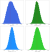 |
Fig. 1. Probability distribution functions for the mass (upper left), age (upper right), mean density (lower left), and radius (lower right) for Kepler-444, obtained using AIMS. The vertical lines indicate the position of the best model obtained from a simple scan of the grid. |
An illustration of the impact of using different observational constraints is shown in Fig. 2, where we show the results for models built using either the individual frequencies or the frequency ratios besides the nonseismic parameters listed above. As can be seen, some differences between the model frequencies are observed. The model built fitting the individual frequencies included the Ball et al. (2016) correction for the surface effects. We plot here the uncorrected frequencies for this model to illustrate the impact of the surface correction at the higher frequencies. The amplitude of the empirical surface correction is actually much larger than the observational uncertainties on the individual frequencies themselves. The model built using the frequency ratios does not show the same behavior, but shows a slightly worse agreement at low frequencies.
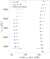 |
Fig. 2. Echelle diagram for Kepler-444. The observational values are plotted in blue while the green and red symbols refer to two reference models computed using different seismic constraints. Δν is the average large frequency separation (determined here following a least-square fitting of the individual large frequency separations for all modes). |
However, both models have similar fundamental parameters. The main difference is in the estimated precision of these parameters. Using the individual frequencies as direct constraints improves the precision by a factor 2.5 compared to that obtained when using the frequency ratios. Similar effects were seen in Rendle et al. (2019) when testing AIMS on theoretical models and on the Sun. In practice, such precision is unrealistic as the individual frequencies are strongly affected by the surface corrections. Moreover, from a theoretical point of view, each frequency does not provide independent information on the internal structure of the star as the link between pulsation frequencies and the internal structure of a star can be expressed using only a few parameters1. Consequently, directly using them as constraints in a stellar model selection procedure will lead to an overestimated precision on the inferred stellar model parameters. As we see below, changing the physical ingredients may lead to modifications of the fundamental parameters at a non-negligible order of magnitude with respect to the precision of inferences from Kepler data. This casts some doubt on the level of precision announced by the modeling of the individual frequencies.
This first step of modeling using AIMS allowed us to derive a limited subspace of stellar parameters on which additional investigations can then be attempted with local minimization techniques. Therefore, to fully explore the dependences of the derived stellar parameters on the model input physics, we carried out an additional exploration of the parameter space using a Levenberg-Marquardt algorithm. This allowed us to refine the results obtained with the global minimization and compute a wide range of models on the fly, using different physical ingredients.
2.2. Local minimization and impact of model ingredients
We considered a wide range of physical ingredients for the models built for the local analysis using the Levenberg-Marquardt algorithm. For the equation of state, we tested the CEFF (Christensen-Dalsgaard & Däppen 1992), FreeEOS (Irwin 2012), and OPAL (Rogers & Nayfonov 2002) equations of state. For the abundances, we tested the AGSS09 (Asplund et al. 2009), GN93 (Grevesse & Noels 1993), and α-enriched AGSS09 tables with [α/Fe] = 0.2 and 0.3. We considered various opacity tables, namely the OPAL (Iglesias & Rogers 1996) and OPLIB tables (Colgan et al. 2016) for a scaled solar mixture, as well as OPAL tables for α-enriched abundances. We also investigated the impact of varying the hypotheses linked to the transport of chemicals by microscopic diffusion, namely the use of the Paquette et al. (1986) screened potentials as well as the impact of the hypothesis of partial ionization, which ought to have an impact on the evolutionary track (Schlattl 2002). We also varied the outer boundary conditions of the models, testing the impact of Krishna Swamy (1966), Vernazza et al. (1981) and Eddington gray T(τ) relations on the results. The convection theory of Canuto et al. (1996) was also used in a model and compared to the classical mixing-length theory, implemented in CLES following the approach described in Cox & Giuli (1968). We used a solar-calibrated mixing length parameter for all our minimizations, adapting it accordingly to the outer boundary conditions and convection formalism used in the modeling.
The fundamental parameters obtained using these various physical ingredients are summarized in Table 12. The minimization procedure was carried out starting from various initial conditions, inside and outside of the range provided by AIMS, for the different sets of ingredients, using the same set of classical constraints as in AIMS and the frequency ratios. Overall, the Levenberg-Marquardt minimization confirmed the values provided with the MCMC approach.
Parameters of the models of Kepler-444 computed in this study.
Some minimizations were also performed including αMLT as one of the free parameters. We found that the value remained close to solar and did not significantly improve the fit. The degeneracy of the problem did not allow us to find an “optimal” value of αMLT from the modeling. Also, following the analytical formulas of Magic et al. (2015) would lead to a slight increase of the mixing-length parameter with respect to the solar value. This would lead the optimal model to lie within the “higher-mass” range of the interval we find.
First, we notice that the variations induced by the physical parameters on the Levenberg-Marquardt results remain limited, although not negligible. For most cases, they are smaller than the uncertainties given by AIMS and those reported in Campante et al. (2015). This is not surprising, but it should be noted that some of these variations are still significant with respect to the uncertainties provided by AIMS. The largest variations are observed when using the Canuto et al. (1996) formalism of convection3, leading to a significantly lower mass. Unsurprisingly, the OPLIB opacities also significantly alter the modeling result, leading to a lower mass value. Changing the solar mixture or using α-enhanced mixtures does not significantly alter the parameters, as already noted by Campante et al. (2015). However, in our test cases, using α-enhanced tables lead to a much better fit of nonseismic constraints while keeping the agreement with the seismic data.
On a sidenote, given the age and low metallicity of Kepler-444, the helium abundance is naturally bound to be close to the primordial abundance. In our study, we considered the primordial helium values determined by Peimbert et al. (2016) and Fernández et al. (2018) of respectively YP = 0.2446 ± 0.0029 and YP = 0.244 ± 0.006 as lower boundaries for our models. This value actually imposes an upper boundary on the mass of Kepler-444 and from our investigations using a solar-calibrated mixing-length, models of 0.77 M⊙ and more could only agree with seismic data if their initial helium abundance was lower than the primordial value. This higher-mass regime could potentially be reached if a significant modification was made to the radiative opacities or if one uses a nonsolar calibrated mixing-length. This is for example the case if we use a mixing-length value calibrated from the 3D simulations, following the formulas of Magic et al. (2015).
The fundamental parameters found after these investigations confirm the results of Campante et al. (2015). However, our thorough modeling has shown that changes in the physical ingredients of the stellar model could easily induce variations of the determined stellar fundamental parameters at a level significant for the reported observational uncertainties of Kepler data. This implies that fundamental parameter determinations of Kepler targets must consider the systematics of the model uncertainties in order to provide reliable precision estimates to other fields of astrophysics, as is attempted in Table 3 of Silva Aguirre et al. (2015). In the particular case of Kepler-444, the modeling with AIMS using the frequency ratios can provide more realistic estimates of the uncertainties on the fundamental parameters stemming from the observational uncertainties. These can be assessed from Fig. 1. To these estimates, we can add the maximal systematic variations found from the tests using various physics to have a more robust precision4. From a simple arithmetic average of the values obtained from the Levenberg-Marquardt fits, we determine the fundamental parameters of Kepler-444 to be 0.749 ± 0.045 M⊙, 0.750 ± 0.015 R⊙ and 11.45 ± 1.0 Gyr for the mass, radius and age, respectively. In this last step, we have increased the error bars to take into account the dispersion we saw when varying the physical ingredients in our detailed analysis with the Levenberg-Marquardt minimization algorithm. We remain conservative with respect to the error bars provided by the Levenberg-Marquardt algorithm itself, which are typically a factor two lower, for all quantities (i.e., ≈0.02 M⊙ for mass, ≈0.007 R⊙ for radius and ≈0.5 Gyr for age). Here, we have added the dispersion between the various models in Table 1 to these uncertainties to obtain an increased precision for the stellar parameter determinations. We also note that these values are in good agreement with those found using AIMS.
In Sect. 3, we carry out mean density inversions and compute a second set of models using a similar strategy to that shown in this section to determine updated values of the fundamental parameters. These values are given in Sect. 3.2. Moreover, we will discuss in Sect. 4 some additional aspects of the modeling that have been brought to light by our extended modeling procedure.
3. Inversions for stellar structure
To further increase the thoroughness of the seismic modeling of Kepler-444, we supplemented our forward approach with seismic inversions of global quantities, so-called indicators, as in Reese et al. (2012), Buldgen et al. (2015a,b,2018). In the specific case of Kepler-444, we limit ourselves to inversions of the mean density. The reason of these limitations is found in the quality of the seismic data. Indeed, in the specific case of Kepler-444, the high radial order of the observed modes and the uncertainties on the frequency values do not allow us to use other quantities such as the tu or the SEnv indicators (unlike the case of the study of the 16Cyg binary system in Buldgen et al. 2016a,b). We performed tests on one core condition indicator, denoted SCore in Buldgen et al. (2018) and found that it confirmed the properties of the models already fitting the frequency ratios.
The inversions of structural indicators are based on the linear approximation between relative frequency differences and structural corrections derived by Dziembowski et al. (1990) and used for helioseismic inversions. The linear formulation of the inverse problem results from the variational principle of adiabatic stellar oscillations (Lynden-Bell & Ostriker 1967). In this context, the linear relation writes
with  being the structural kernel functions, related to the reference model used for the inversion and the eigenfunctions of the oscillation modes. Here, ℱ is the function related to the surface effect correction and the relative differences in quantities denoted as “δ” follow the definition
where the subscript “ref” is related to quantities of the reference model (frequencies, sound speed or density for example) and the subscript “obs” denotes the quantities related to the observed star. The goal of the inversion procedure is to estimate the observed structural quantities (s1, obs, s2, obs) from a given set of observed frequencies (ν1, obs, ν2, obs).
In practice, Eq. (2) can be written for a large variety of structural variables, for which corrections can then be inferred. The variables will always come in pairs, such as for example: (c2, ρ), (c2, Γ1), (ρ, Y), (u, Y), or (S5/3, Y) with 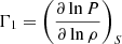 ,
,  the squared adiabatic sound speed, with P the local pressure and ρ the local density, Y the helium mass fraction,
  and
and  , a proxy of the entropy of the stellar material. In these last three cases, one assumes the equation of state of the stellar material to be known and thus the relative differences in Γ1 can be developed linearly according to
with Z being the heavy elements abundance. In practice, this last term is often omitted in asteroseismic inversions due to the low amplitude of the metallicity differences compared to the other terms. In general, the use of Γ1 or Y as a secondary variable can help to mitigate the amplitude of the cross-term of the inversion and thus increase the accuracy of the inference (see Buldgen et al. 2015b, for a discussion in the case of asteroseismic inversions).
The surface correction term, ℱ, is considered to be a slowly varying function of the frequency and modeled using empirical formulations (see e.g. Ball & Gizon 2014; Sonoi et al. 2015; Ball et al. 2016). In the following section, we test various approaches to quantify the robustness of our results with respect to the surface corrections.
In this study, we use the Substractive Optimally Localized Averages (SOLA) inversion technique (Pijpers & Thompson 1994) to determine structural indicators for Kepler-444. Other approaches have also been used to solve the inverse problem, complementary to that using the variational formulation (see e.g. Roxburgh 2002; Roxburgh & Vorontsov 2002a,b; Appourchaux et al. 2015). These could potentially provide a strong complement to the linear formalism, which is intrinsically limited and can be model-dependent.
3.1. Mean density inversions
Mean density inversions have been formalized by Reese et al. (2012) as a way to exploit individual oscillation frequencies to extract this key quantity from seismic observations in a model-independent way. The method has since been thoroughly tested (Reese et al. 2012; Buldgen et al. 2015a, 2019) and applied to various cases (see Buldgen et al. 2016a,b, 2017). The inversion procedure is based on Eq. (2), written for the (ρ, Γ1) structural pair.
The inversion for the mean density using the SOLA technique is carried out by defining a target function related to the integral definition of the mean density,
From Eq. (5), nondimensionalizing the integral and slightly modifying the expression gives the definition of the target function of the inversion:
with x = r/R being the normalized radial position of an element of stellar matter, R the photospheric radius, and ρR = M/R3, with M the mass of the star.
Following these definitions, the cost function of the SOLA inversion then reads
![$$ \begin{aligned} \mathcal{J} _{\bar{\rho }}(c_{i})=&\int _{0}^{1}\left[K_{\mathrm{Avg} } - \mathcal{T} _{\bar{\rho }}\right]^{2}\mathrm{d}x + \beta \int _{0}^{1}\left( K_{\mathrm{Cross} }\right)^{2}\mathrm{d}x \nonumber \\&+ \lambda \left[ 2 -\sum _{i}c_{i} \right] + \tan \theta \frac{\sum _{i}\left(c_{i}\sigma _{i}\right)^{2}}{\langle \sigma ^{2}\rangle } + \mathcal{F} _{\mathrm{Surf} }(\nu ). \end{aligned} $$](/articles/aa/full_html/2019/10/aa36126-19/aa36126-19-eq12.gif)
In Eq. (7), we have defined the averaging and cross-term kernels of the inversion, which are related to the structural kernels
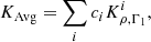
We have also introduced the so-called trade-off parameters, β and θ, which are used to adjust the balance between fitting the target function, mitigating the amplitude of the cross term contribution of the inversion and the amplification of observational error bars of the individual frequencies (σi). In addition, we have defined  with N the number of observed frequencies and introduced the inversion coefficients ci and a Lagrange multiplier λ.
The third term of Eq. (7) stems from homologous reasoning (see Reese et al. 2012), which defines a crude nonlinear generalization of the method to determine  , the inverted mean density, from
with  the mean density of the reference model and
  the relative differences between the observed and theoretical frequencies defined as in Eq. (2). In this study, we apply the nonlinear formula to all inversion procedures. Using this formalism, the error propagation of the inversion is also modified and thus the uncertainties on the inverted mean density are given by
The last term of Eq. (7) is related to the correction of surface effects. Various procedures have been suggested in the literature to tackle this tedious issue, which results from the intrinsic nature of solar-like oscillations. In helioseismology, the surface correction function is defined as a series of Legendre polynomials, which can go up to order six or seven depending on the considered dataset. This approach is however not suitable for asteroseismic applications, where the number of observed individual frequencies is insufficient to simultaneously fit the target function, mitigate the cross-term and the error propragation, while also reproducing the expected trend of the surface correction.
Consequently, early mean density inversions limited the surface correction to a linear term. However, comparisons in hare-and-hounds exercises showed that this approach was not robust and could bias the inverted values (Reese et al. 2016). In practice, more recent parametrizations of the surface effect are favored and included in the inversion procedure. Buldgen et al. (2019) investigated the effects of these corrections on mean density inversions for red giant stars and found that they could induce slight modifications of the results. Moreover, they also investigated the impact of nonadiabatic effects of the frequencies on the inverted results.
In this study, we test various approaches for the correction of the surface effect. The first one is to directly introduce the formulation of Ball et al. (2016) or Sonoi et al. (2015) in the SOLA cost-function and consider the coefficients of these correction laws to be free parameters to be determined by the inversion procedure, as is done for the classical helioseismic correction approach. Another approach is to correct a priori for the surface effects using either the empirical law depending on Teff and log g described in Sonoi et al. (2015) or using pre-determined values of the coefficients of the Ball et al. (2016) formula.
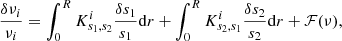
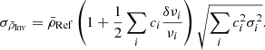
In the case of Kepler-444, we computed the mean density inversions for a wide range of reference models described in Sect. 2, varying the correction for the surface effects. The inversion results are illustrated in Fig. 3. As can be seen, the inversion is robust well within 1%, despite changing the reference model and the surface correction applied to the frequencies. Moreover, we found that the largest variations of the inversion results are observed when changing the surface correction law. More specifically, implementing directly the Ball et al. (2016) surface correction as additional free parameters leads to the largest deviations, as well as a significant reduction of the quality of the averaging kernel. This confirms the results already found in Buldgen et al. (2019) for red giant stars.
 |
Fig. 3. Results of mean density inversion for various reference models and surface corrections plotted against the masses of the reference models. The vertical lines indicate the limiting values considered to be consistent with the inversion procedure. |
In Fig. 3, the effect of the Ball et al. (2016) surface correction law can be seen for the inverted points with larger error bars that are above 2.5 g cm−3. Typically, using the Ball et al. (2016) surface correction induces a shift of 0.008 g cm−3, whereas the Sonoi et al. (2015) formula induces a shift of 0.005 g cm−3. Both methods shift the inversion results in the same direction, namely towards higher mean density values. The spread of values obtained from the model dependency is slightly smaller, typically of the order of 0.004 g cm−3 and located between 2.486 and 2.490 g cm−3.
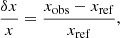
Another way of assessing the robustness of the inversion is to inspect the behavior of the averaging and cross-term kernels. This is done in Fig. 4 for Model1 of Table 1. The agreement with the target function and the amplitude of the cross-term is very similar to what has been obtained in previous studies analyzing the accuracy and robustness of mean density inversions5. Looking at Fig. 3, we can state that, by using various reference models and surface effect corrections, the mean density inversion still provides a very accurate and robust determination of the mean density of Kepler-444, beyond what would have been achievable by standard forward modeling.
 |
Fig. 4. Left panel: target function of the mean density inversion (green) and averaging kernel of the inversion (blue) as a function of the adimensional stellar radius. Right panel: cross-term kernel of the mean density inversion (blue) and its target value (zero; green), as a function of the adimensional stellar radius. |
Overall, the behavior of the inversion is satisfactory. We therefore conservatively assess that the mean density of Kepler-444 must lie within 2.496 ± 0.012 g cm−3. This result agrees with the value reported by Campante et al. (2015), who found 2.493 ± 0.028 g cm−3. Unsurprisingly, the inversion technique, making full use of the information of the frequency spectrum to determine the value of the indicator, provides a more precise estimate of the sought integrated quantity, by a factor two in this instance. This value can then be used to constrain stellar and planetary parameters to a higher degree of precision. We note that some of the models computed in Sect. 2 already fitted the mean density within its uncertainties.
On a sidenote, it is also worth noticing that even the mean density inversions show some degree of model-dependency, and, to an even greater degree, a dependency on the surface correction approach used when computing the inversion. This confirms that asteroseismic inversions, at least within the linear formalism6, are not fully model-independent. Consequently, assessing their true precision cannot be done by merely propagating the observational error bars of the individual frequencies derived from Eq. (11).
3.2. Revised forward modeling and impact on planetary parameters
Thanks to the very precise determination of the mean density of Kepler-444 from the inversion procedure, we can re-run a set of models using the Levenberg-Marquardt minimization and determine updated values for the fundamental parameters. We used the same set of constraints as in Sect. 2, but reduced the uncertainties on the mean density from 0.05 to 0.012 g cm−3, in agreement with the inversion procedure. As stated in Sect. 3.1, some of the reference models already agreed with the inverted mean density within the precision of the inversion procedure. However, this was not the case for all models, particulary those responsible for the largest spread in fundamental parameters such as those using the Canuto et al. (1996) formalism of convection or the OPLIB opacity tables. Whenever possible, we used the α-enriched opacities and abundance tables to compute this second set of models.
While the mean values of the fundamental parameters did not change significantly, recomputing the whole set of models using this more accurate value of the mean density allowed for a higher precision of their determination. The final values for this consolidated stellar seismic modeling are summarized in Table 2. For this last set of values, we have kept the error bars conservative and have combined the errors from the remaining dispersion between the various models and those from the uncertainties on the observational constraints. We note that these final values are in excellent agreement with those found in Campante et al. (2015); they are however, slightly more precise, as Campante et al. (2015) report a 0.043 M⊙ uncertainty on mass, a 0.013 R⊙ uncertainty on radius, and a +0.91 and −0.99 Gyr uncertainty on age. This is likely a consequence on the improved precision on the stellar mean density as a result of the use of the seismic inversion as we used a slightly larger uncertainty on the luminosity than Campante et al. (2015), as a result of the disagreements in Teff between the recent determinations found in the literature.
Improved stellar parameter values for Kepler-444.
Using these updated stellar parameters, we revise the most recent estimates of the planetary parameters derived by Mills & Fabrycky (2017). These results are summarized in Table 3 and we illustrate the position of planet (e) and (f) on a mass-radius diagram in Fig. 5.
Revised planetary parameters for Kepler-444 system.
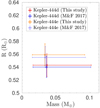 |
Fig. 5. Comparisons between the masses and radii of Kepler-444d and Kepler-444e determined from this study and the study of Mills & Fabrycky (2017). |
As could already be guessed from comparisons with Campante et al. (2015), we find no significant modifications to the values of the planetary masses and radii. Changes in the precision of the planetary radii are minimal, due to the reduced changes on the precision on the stellar radii. Similarly, the uncertainties on the mass values from Mills & Fabrycky (2017) are largely dominated by the uncertainties on the TTV data. Thus, revising the stellar parameters has little to no impact on the planetary masses. However, other systems where the uncertainties on the host star dominate could significantly benefit from a detailed seismic study such as the one carried out here. Consequently, we find that Kepler-444e and Kepler-444f remain excellent candidates of ocean planets. As noted by Mills & Fabrycky (2017), future observations with PLATO may provide the additional data required to more precisely determine the masses and radii of the planets orbiting Kepler-444, confirming their nature.
4. Survival of a convective core in Kepler-444
In Sect. 2, we show that the spread of the fundamental parameters we obtained remained small, but not negligible, compared to the uncertainties obtained from AIMS and the Levenberg-Marquardt minimization using one set of physical ingredients. The extended testing procedure we used allowed us to conclude that the derived parameters are robust. However, further investigations have led us to consider whether the accuracy of the fit could be further improved. It appeared that, despite converging systematically on the same results, all models presented a slight disagreement in the frequency ratios. We illustrate this effect in the right panel of Fig. 6, where we show in red the results for a best-fit model “Model11” of Table 1. One can clearly see that the higher range of frequency ratios is not well fitted by this model. This disagreement is present in all models considered, regardless of the physical ingredients used to fit the ratios.
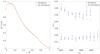 |
Fig. 6. Left panel: adimensional sound speed profile as a function of the adimensional stellar radius for two models (Model12 and Model13 in Table 1) of Kepler-444 with (green) and without (red) overshooting. Right panel: frequency ratios as a function of the observed radial frequency. The upper symbols are related to the r0, 2 ratios while the lower ones are related to the r0, 1 ratios. The blue symbols are related to the observed values of the ratios while their theoretical counterparts are plotted in green and red for Model13 and Model12 with and without overshooting, respectively. |
One solution to improve the agreement with these seismic indices is to include a moderate amount of overshooting in the modeling (typically αOv ≈ 0.18HP, with HP being the pressure scale height defined as  ). The results for such a model of Kepler-444, including overshooting, namely Model13 of Table 1, are illustrated in green in the right panel of Fig. 6. The variation in χ2 is relatively small, as one goes from 1.24 for the reduced χ2 of a model without overshooting to 0.99 for a model including overshooting. The largest contributions to the χ2 in the case with overshooting stem from the r0, 1 ratio of the n = 21 and n = 20 modes for the seismic constraints and from Teff for the nonseismic constraints. We note however that the values of Teff tend to favor the revised determination of Mack et al. (2018), but no firm conclusions can be drawn given the relatively large uncertainties.
Further increasing the extent of the mixed region leads, in this case, to the survival of the convective core on the main sequence for the model of Kepler-444 and significantly alters its present-day sound speed profile. In the left panel of Fig. 6, we illustrate the sound speed profile of two optimal models for Kepler-444 with and without a surviving convective core on the main sequence. In the left panel of Fig. 7, we illustrate the extent of the convective core as a function of the age of the model. As can be seen, including overshooting helps the convective core to maintain itself for a significant portion of the main sequence, despite the very low mass of the star.
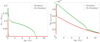 |
Fig. 7. Left panel: mass of the convective core expressed as a fraction of the stellar mass in Model13 (with overshooting, green) and Model12 (without overshooting, red) of Kepler-444 as a function of age. Right panel: central 3He abundance as a function of age for Model12 (red) and Model13 (green) of Kepler-444. |
Such a situation, although unexpected at first glance, is not uncommon, as Deheuvels et al. (2010) reported a similar feature in HD203608, a low-mass low-metallicity, and alpha-enriched solar-like oscillator observed by CoRoT. In the case of Kepler-444, the signature of the convective core appears fainter. To further confirm this result, we computed the so-called small frequency spacing used by Deheuvels et al. (2010) to discriminate models without overshooting and tested whether these indices could also keep trace of the survival of a convective core in Kepler-444. We found that the small spacings were not as constraining as the frequency ratios. Their behavior could be altered by other ingredients such as the upper boundary conditions and the use of the Canuto et al. (1996) formalism of convection in the envelope. The fact that we were not able to see the trace of the convective core in the small spacings might stem from the fact that it has already disappeared in Kepler-444 at the time of observation. This was not the case in HD203608, which still bears a convective core according to the seismic analysis of Deheuvels et al. (2010).
This behavior can also be understood by looking at the left panel of Fig. 6, illustrating the differences in sound speed for a model with and without a long-lasting convective core of Kepler-444. By comparing this illustration to Fig. 2 of Deheuvels et al. (2010), we can see that the sharp signature of the convective core that is present in HD203608 is almost erased in Kepler-444, due to the effects of microscopic diffusion. Following the second-order asymptotic developments of Provost et al. (1993), Deheuvels et al. (2010) explained that the small spacing would be sensitive to sharp variations in the sound speed profile. Since this variation has disappeared in Kepler-444, it is not surprising that the small spacings are very similar between models with and without a surviving convective core on the main sequence. The slope of the sound speed profile in the core is still however very different between the two models, as can be seen from the left panel of Fig. 6. This explains why the frequency ratios, indicative of the sound speed gradient in deep layers, provide a clearer diagnostic of the core history of Kepler-444.
By further increasing the values of the overshooting parameter, one can make the convective core survive even longer. However, attempts with larger values, that could lead to the presence a convective core in Kepler-444 at its current age, disagree with the observed ratios. When attempting to carry out minimizations with such larger values, the disagreement with the frequency ratios led to models for which the core had disappeared at the observation time, thus agreeing with the observed frequency ratios as models with lower overshooting values, but larger discrepancies for global parameters such as the mean density, luminosity, log g and, [Fe/H].
The physical explanation behind the survival of the convective core in such circumstances has been extensively detailed in Deheuvels et al. (2010). In the case of Kepler-444, tests using models built using seismic and classical constraints with and without overshooting indicate a similar origin as in the case of HD203608. In Fig. 7, we illustrate the evolution of the convective core in a model of Kepler-444 with and without overshooting and show its link to the evolution of the abundance of 3He in the central regions.
The evolution and survival of the convective core in the model is indeed clearly due to the 3He fusion reactions. Without overshooting, the abundances quickly reach an equilibrium value for the [3He/H] ratio, and the ppI chain achieves equilibrium. If overshooting is included during the evolution, the additional mixing provides more 3He in the central regions and extends the duration of nuclear burning out of equilibrium. Due to the much higher temperature sensitivity of out-of-equilibrium 3He burning, the generated energy flux cannot be evacuated by radiation alone and the convective core remains for longer during the main sequence, up to an age of ≈8 Gyr. However, as the extension of the convective core is smaller than the region where nuclear burning occurs the [3He/H] ratio reaches its equilibrium value after a while. The convective core then quickly disappears and nuclear burning now occurs in radiative equilibrium conditions. This can be seen in Fig. 7, where the slope of the central 3He abundance changes drastically at the time when the convective core disappears. From inspection of the energy generation rates, we can also confirm that the CNO cycle did not play any part in sustaining the convective core, the central temperatures being too low for it to have a significant role during the evolution.
While additional mixing is essential to sustain the convective core for an extended period on the main sequence, its origin is not necessarily only linked to “convective overshooting”7. Efficient mixing may also occur if, at the beginning of the main sequence, the star rotates almost in a solid way. In those conditions, transport of chemicals by the meridional circulation may also provide an additional source of 3He that will provide material for 3He burning and thus sustain the transitory convective core. This phenomenon is also mentioned in Roxburgh (1985) to explain a potential mechanism to sustain an efficient mixing in the solar core. The phenomenon was linked to the so-called “solar-spoon” mechanism presented by Dilke & Gough (1972) which was extensively discussed (see e.g. Ulrich & Rood 1973; Christensen-Dalsgaard et al. 1974; Unno 1975; Shibahashi et al. 1975, for a few references) and also investigated for Population III stars (Sonoi & Shibahashi 2012). In the latter case, the mixing results from the transport of chemicals by the nonlinear gravity modes generated by a form ϵ-mechanism due to the nuclear burning of 3He. Seismic data alone are not sufficient to distinguish between the two cases, or to confirm that a combination of both effects is at play. To that end, additional constraints on the lithium and beryllium abundances may provide an indication of the efficiency of rotational mixing in the early stages of evolution and thus inform us on whether rotation would be able to provide the required mixing of chemicals.
As seen from the seismic modeling results, the survival of the convective core does not affect the global stellar parameters. The main reason is that its extension is smaller than the region of nuclear burning, and therefore, it does not significantly modify the evolutionary track of Kepler-444. However, it could potentially affect the angular momentum transport properties and lead to discrepancies in later evolutionary stages. This aspect still remains rather speculative and will be further investigated in future studies.
5. Conclusion
Here, we carried out a thorough modeling of Kepler-444 using updated parallax values from Gaia DR2 (Gaia Collaboration 2018) as well as updated spectroscopic parameters (Mack et al. 2018). We combined global and local forward modeling approaches to structural inversion techniques to derive robust fundamental parameters for this exoplanet-host star. To do so, we tested a wide range of physical ingredients and analyzed the spread of the fundamental parameters obtained. Amongst others, we investigated the impact of α-enriched abundance tables and their corresponding opacities rather than solar-scaled abundances. Overall, we confirm the results of Campante et al. (2015) and also find relatively good agreement with the results of Silva Aguirre et al. (2015). We note, however, that the luminosity derived from the Gaia parallax is significantly higher than those obtained in these studies, especially if we consider recent spectroscopic constraints. Some of these discrepancies stem from the Gaia parallax itself, but also from differences in the effective temperature values reported in the literature. The case of Kepler-444 is therefore a good illustration of where the use of the very precise Gaia parallaxes can be limited by other spectroscopic constraints.
In addition to forward modeling, we used mean density inversions to provide a very precise, nearly model-independent value for the stellar mean density of 2.496 ± 0.012 g cm−3. This value was then used as a direct constraint for a second set of forward modeling, combined with the other classical and seismic constraints used in the modeling. Using this two-step approach, we determine the mass, radius and age of Kepler-444 to be 0.754 ± 0.030 M⊙, 0.753 ± 0.010 R⊙ and 11.00 ± 0.8 Gyr. As these parameters are very similar to those of Campante et al. (2015), we find no significant modifications of the planetary parameters using our modeling results.
However, we have determined that Kepler-444 bore a convective core during a significant fraction of its main-sequence evolution, as was found by Deheuvels et al. (2010) for the CoRoT target HD203608. The origin of the convective core in the case of Kepler-444 is similar to the case of HD203608 and can be linked to the nuclear burning of 3He out of equilibrium. The absence of equilibrium conditions for a prolongated portion of time after the ZAMS is due to an additional mixing, providing more nuclear fuel for the He3 combustion. The origin of this mixing is unclear and could be due to rotation, overshooting, or even nonlinear gravity modes, although this latter case seems less plausible considering the stability analyses of Sonoi & Shibahashi (2012). The seismic data alone cannot disentangle between these processes. Promising indicators of the efficiency of rotational mixing in the early stages that could help lift this degeneracy are the lithium and beryllium abundances, yet to be determined in the case of Kepler-444. So far, using seismology, we are however able to estimate the lifetime of the convective core to be of around 8 Gyr.
The survival of the convective core, as noted by Deheuvels et al. (2010), does not affect the fundamental parameters of the star, but it could play a key role in the angular momentum transport in later stages of evolution. A thorough modeling of the star including rotation and transport by magnetic instabilities as in Eggenberger et al. (2010) will be undertaken in a future paper. These transport prescriptions will then be used to characterize the dynamical properties of the system, following the approach of Privitera et al. (2016a) and Rao et al. (2018). In turn, such detailed studies will pave the way for joint analyses of the stellar-planetary system as a whole, including atmospheric characterizations and the change of these properties when coupled to seismically calibrated nonstandard stellar evolution models.
With the advent of TESS and PLATO, such synergies between exoplanetology and asteroseismology will be further reinforced. For the best targets, a thorough modeling and investigation of the history of the system with respect to the evolution of its host star can be foreseen. In this series of papers, we will illustrate these possibilities for a promising target observed by Kepler. In the specific case of Kepler-444, Mills & Fabrycky (2017) estimate that PLATO observations could help to significantly reduce the current uncertainties on the planetary masses.
MLT denotes the use of the classical mixing-length theory as in Cox & Giuli (1968), whereas CM denotes the use of the Canuto et al. (1996) formalism of convection. PartIon implies the use of partial ionization in the treatment of microscopic diffusion, OV implies the inclusion of convective overshooting in the core. VAL-C and Krishna-Swamy denote the use of a Vernazza et al. (1981) and a Krishna Swamy (1966)T(τ) relations.
Explicitely, we use here the expression of the convective flux by Canuto et al. (1996) and the expression of the scale length by Canuto & Mazzitelli (1991).
The value of the cross-term is multiplied by the relative differences in Γ1 between the reference model and the target, leading typically to negligible errors in the procedure (see Reese et al. 2012; Buldgen et al. 2015a, for a discussion).
Although similar issues have been reported in Appourchaux et al. (2015) for nonlinear inversion.
Acknowledgments
This work is sponsored by the Swiss National Science Foundation (project number 200020-172505). M.F. is supported by the FNRS (“Fonds National de la Recherche Scientifique”) through a FRIA (“Fonds pour la Formation à la Recherche dans l’Industrie et l’Agriculture”) doctoral fellowship. S.J.A.J.S. is funded by the Wallonia-Brussels Federation ARC grant for Concerted Research Actions. A.M. and J.M. acknowledge support from the ERC Consolidator Grant funding scheme (project ASTEROCHRONOMETRY, G.A. n. 772293). We gratefully acknowledge the support of the UK Science and Technology Facilities Council (STFC). V.B. acknowledges by the Swiss National Science Fundation (SNSF) in the frame of the National Centre for Competences in Research PlanetS and has received fundings from the European Research Council (ERC) under the European Union’s Horizon 2020 research and innovation programme (project Four Aces; grant agreement number 724427). This article used an adapted version of InversionKit, a software developed within the HELAS and SPACEINN networks, funded by the European Commissions’s Sixth and Seventh Framework Programmes.
References
- Appourchaux, T., Antia, H. M., Ball, W., et al. 2015, A&A, 582, A25 [NASA ADS] [CrossRef] [EDP Sciences] [Google Scholar]
- Asplund, M., Grevesse, N., Sauval, A. J., & Scott, P. 2009, ARA&A, 47, 481 [NASA ADS] [CrossRef] [Google Scholar]
- Baglin, A., Auvergne, M., Barge, P., et al. 2009, in IAU Symposium, eds. F. Pont, D. Sasselov, & M. J. Holman, 253, 71 [Google Scholar]
- Bailer-Jones, C. A. L., Rybizki, J., Fouesneau, M., Mantelet, G., & Andrae, R. 2018, AJ, 156, 58 [NASA ADS] [CrossRef] [Google Scholar]
- Ball, W. H., & Gizon, L. 2014, A&A, 568, A123 [NASA ADS] [CrossRef] [EDP Sciences] [Google Scholar]
- Ball, W. H., Beeck, B., Cameron, R. H., & Gizon, L. 2016, A&A, 592, A159 [NASA ADS] [CrossRef] [EDP Sciences] [Google Scholar]
- Batalha, N. M., Borucki, W. J., Bryson, S. T., et al. 2011, ApJ, 729, 27 [NASA ADS] [CrossRef] [Google Scholar]
- Bazsó, Á., Pilat-Lohinger, E., Eggl, S., et al. 2017, MNRAS, 466, 1555 [NASA ADS] [CrossRef] [Google Scholar]
- Borucki, W. J., Koch, D., Basri, G., et al. 2010, Science, 327, 977 [NASA ADS] [CrossRef] [PubMed] [Google Scholar]
- Bourrier, V., Ehrenreich, D., Allart, R., et al. 2017, A&A, 602, A106 [NASA ADS] [CrossRef] [EDP Sciences] [Google Scholar]
- Brewer, J. M., Wang, S., Fischer, D. A., & Foreman-Mackey, D. 2018, ApJ, 867, L3 [NASA ADS] [CrossRef] [Google Scholar]
- Buldgen, G., Reese, D. R., Dupret, M. A., & Samadi, R. 2015a, A&A, 574, A42 [NASA ADS] [CrossRef] [EDP Sciences] [Google Scholar]
- Buldgen, G., Reese, D. R., & Dupret, M. A. 2015b, A&A, 583, A62 [NASA ADS] [CrossRef] [EDP Sciences] [Google Scholar]
- Buldgen, G., Reese, D. R., & Dupret, M. A. 2016a, A&A, 585, A109 [NASA ADS] [CrossRef] [EDP Sciences] [Google Scholar]
- Buldgen, G., Salmon, S. J. A. J., Reese, D. R., & Dupret, M. A. 2016b, A&A, 596, A73 [NASA ADS] [CrossRef] [EDP Sciences] [Google Scholar]
- Buldgen, G., Reese, D., & Dupret, M.-A. 2017, Eur. Phys. J. Web Conf., 160, 03005 [NASA ADS] [CrossRef] [EDP Sciences] [Google Scholar]
- Buldgen, G., Reese, D. R., & Dupret, M. A. 2018, A&A, 609, A95 [NASA ADS] [CrossRef] [EDP Sciences] [Google Scholar]
- Buldgen, G., Rendle, B., Sonoi, T., et al. 2019, MNRAS, 482, 2305 [NASA ADS] [CrossRef] [Google Scholar]
- Campante, T. L., Barclay, T., Swift, J. J., et al. 2015, ApJ, 799, 170 [NASA ADS] [CrossRef] [Google Scholar]
- Campante, T. L., Santos, N. C., & Monteiro, M. J. P. F. G. 2018, Asteroseismology and Exoplanets: Listening to the Stars and Searching for New Worlds (Springer International Publishing AG), 49 [Google Scholar]
- Canuto, V. M., & Mazzitelli, I. 1991, ApJ, 370, 295 [NASA ADS] [CrossRef] [Google Scholar]
- Canuto, V. M., Goldman, I., & Mazzitelli, I. 1996, ApJ, 473, 550 [NASA ADS] [CrossRef] [Google Scholar]
- Casagrande, L., & VandenBerg, D. A. 2014, MNRAS, 444, 392 [NASA ADS] [CrossRef] [MathSciNet] [Google Scholar]
- Casagrande, L., & VandenBerg, D. A. 2018a, MNRAS, 475, 5023 [NASA ADS] [CrossRef] [Google Scholar]
- Casagrande, L., & VandenBerg, D. A. 2018b, MNRAS, 479, L102 [NASA ADS] [CrossRef] [Google Scholar]
- Cassisi, S., Potekhin, A. Y., Pietrinferni, A., Catelan, M., & Salaris, M. 2007, ApJ, 661, 1094 [NASA ADS] [CrossRef] [Google Scholar]
- Christensen-Dalsgaard, J., & Däppen, W. 1992, A&ARv, 4, 267 [NASA ADS] [CrossRef] [Google Scholar]
- Christensen-Dalsgaard, J., Dilke, F. W. W., & Gough, D. O. 1974, MNRAS, 169, 429 [NASA ADS] [CrossRef] [Google Scholar]
- Christensen-Dalsgaard, J., Kjeldsen, H., Brown, T. M., et al. 2010, ApJ, 713, L164 [NASA ADS] [CrossRef] [Google Scholar]
- Colgan, J., Kilcrease, D. P., Magee, N. H., et al. 2016, ApJ, 817, 116 [NASA ADS] [CrossRef] [Google Scholar]
- Cox, J. P., & Giuli, R. T. 1968, Principles of Stellar Structure (New York: Gordon and Breach) [Google Scholar]
- Davies, G. R., Handberg, R., Miglio, A., et al. 2014, MNRAS, 445, L94 [NASA ADS] [CrossRef] [Google Scholar]
- Deheuvels, S., Michel, E., Goupil, M. J., et al. 2010, A&A, 514, A31 [NASA ADS] [CrossRef] [EDP Sciences] [Google Scholar]
- Dilke, F. W. W., & Gough, D. O. 1972, Nature, 240, 262 [NASA ADS] [CrossRef] [Google Scholar]
- Dupuy, T. J., Kratter, K. M., Kraus, A. L., et al. 2016, ApJ, 817, 80 [NASA ADS] [CrossRef] [Google Scholar]
- Dziembowski, W. A., Pamyatnykh, A. A., & Sienkiewicz, R. 1990, MNRAS, 244, 542 [NASA ADS] [Google Scholar]
- Eddington, A. S. 1959, The Internal Constitution of the Stars (New York: Dover Publication) [Google Scholar]
- Eggenberger, P., Maeder, A., & Meynet, G. 2010, A&A, 519, L2 [NASA ADS] [CrossRef] [EDP Sciences] [Google Scholar]
- Evans, D. W., Riello, M., De Angeli, F., et al. 2018, A&A, 616, A4 [NASA ADS] [CrossRef] [EDP Sciences] [Google Scholar]
- Ferguson, J. W., Alexander, D. R., Allard, F., et al. 2005, ApJ, 623, 585 [NASA ADS] [CrossRef] [Google Scholar]
- Fernández, V., Terlevich, E., Díaz, A. I., Terlevich, R., & Rosales-Ortega, F. F. 2018, MNRAS, 478, 5301 [NASA ADS] [CrossRef] [Google Scholar]
- Gaia Collaboration (Prusti, T., et al.) 2016, A&A, 595, A1 [NASA ADS] [CrossRef] [EDP Sciences] [Google Scholar]
- Gaia Collaboration (Brown, A. G. A., et al.) 2018, A&A, 616, A1 [NASA ADS] [CrossRef] [EDP Sciences] [Google Scholar]
- Green, G. M., Schlafly, E. F., Finkbeiner, D., et al. 2018, MNRAS, 478, 651 [NASA ADS] [CrossRef] [Google Scholar]
- Grevesse, N., & Noels, A. 1993, in Origin and Evolution of the Elements, eds. N. Prantzos, E. Vangioni-Flam, & M. Casse, 15 [Google Scholar]
- Hadden, S., & Lithwick, Y. 2017, AJ, 154, 5 [NASA ADS] [CrossRef] [Google Scholar]
- Hirsch, L. A., Ciardi, D. R., Howard, A. W., et al. 2017, AJ, 153, 117 [NASA ADS] [CrossRef] [Google Scholar]
- Hobson, M. J., & Gomez, M. 2017, New A, 55, 1 [NASA ADS] [CrossRef] [Google Scholar]
- Huber, D. 2018, Asteroseismology and Exoplanets: Listening to the Stars and Searching for New Worlds (Springer International Publishing AG), 49, 119 [Google Scholar]
- Huber, D., Chaplin, W. J., Christensen-Dalsgaard, J., et al. 2013a, ApJ, 767, 127 [NASA ADS] [CrossRef] [Google Scholar]
- Huber, D., Carter, J. A., Barbieri, M., et al. 2013b, Science, 342, 331 [NASA ADS] [CrossRef] [PubMed] [Google Scholar]
- Iglesias, C. A., & Rogers, F. J. 1996, ApJ, 464, 943 [NASA ADS] [CrossRef] [Google Scholar]
- Irwin, A. W. 2012, Astrophysics Source Code Library [record ascl:1211.002] [Google Scholar]
- Kraus, A. L., Ireland, M. J., Huber, D., Mann, A. W., & Dupuy, T. J. 2016, AJ, 152, 8 [NASA ADS] [CrossRef] [Google Scholar]
- Krishna Swamy, K. S. 1966, ApJ, 145, 174 [NASA ADS] [CrossRef] [Google Scholar]
- Lynden-Bell, D., & Ostriker, J. P. 1967, MNRAS, 136, 293 [NASA ADS] [CrossRef] [Google Scholar]
- Mack, C. E., Strassmeier, K. G., Ilyin, I., et al. 2018, A&A, 612, A46 [NASA ADS] [CrossRef] [EDP Sciences] [Google Scholar]
- Magic, Z., Chiavassa, A., Collet, R., & Asplund, M. 2015, A&A, 573, A90 [NASA ADS] [CrossRef] [EDP Sciences] [Google Scholar]
- Meynet, G., Eggenberger, P., Privitera, G., et al. 2017, A&A, 602, L7 [Google Scholar]
- Mills, S. M., & Fabrycky, D. C. 2017, ApJ, 838, L11 [NASA ADS] [CrossRef] [Google Scholar]
- Paquette, C., Pelletier, C., Fontaine, G., & Michaud, G. 1986, ApJS, 61, 177 [NASA ADS] [CrossRef] [Google Scholar]
- Peimbert, A., Peimbert, M., & Luridiana, V. 2016, Rev. Mex. Astron. Astrofis., 52, 419 [NASA ADS] [Google Scholar]
- Pijpers, F. P., & Thompson, M. J. 1994, A&A, 281, 231 [NASA ADS] [Google Scholar]
- Potekhin, A. Y., Baiko, D. A., Haensel, P., & Yakovlev, D. G. 1999, A&A, 346, 345 [NASA ADS] [Google Scholar]
- Privitera, G., Meynet, G., Eggenberger, P., et al. 2016a, A&A, 591, A45 [NASA ADS] [CrossRef] [EDP Sciences] [Google Scholar]
- Privitera, G., Meynet, G., Eggenberger, P., et al. 2016b, A&A, 593, A128 [NASA ADS] [CrossRef] [EDP Sciences] [Google Scholar]
- Privitera, G., Meynet, G., Eggenberger, P., et al. 2016c, A&A, 593, L15 [Google Scholar]
- Provost, J., Mosser, B., & Berthomieu, G. 1993, A&A, 274, 595 [NASA ADS] [Google Scholar]
- Rao, S., Meynet, G., Eggenberger, P., et al. 2018, A&A, 618, A18 [NASA ADS] [CrossRef] [EDP Sciences] [Google Scholar]
- Rauer, H., Catala, C., Aerts, C., et al. 2014, Exp. Astron., 38, 249 [NASA ADS] [CrossRef] [Google Scholar]
- Reese, D. R., Marques, J. P., Goupil, M. J., Thompson, M. J., & Deheuvels, S. 2012, A&A, 539, A63 [NASA ADS] [CrossRef] [EDP Sciences] [Google Scholar]
- Reese, D. R., Chaplin, W. J., Davies, G. R., et al. 2016, A&A, 592, A14 [NASA ADS] [CrossRef] [EDP Sciences] [Google Scholar]
- Rendle, B. M., Buldgen, G., Miglio, A., et al. 2019, MNRAS, 484, 771 [NASA ADS] [CrossRef] [Google Scholar]
- Ricker, G. R., Winn, J. N., Vanderspek, R., et al. 2015, J. Astron. Telesc. Instrum. Syst., 1, 014003 [NASA ADS] [CrossRef] [Google Scholar]
- Rogers, F. J., & Nayfonov, A. 2002, ApJ, 576, 1064 [Google Scholar]
- Roxburgh, I. W. 1985, Sol. Phys., 100, 21 [NASA ADS] [CrossRef] [Google Scholar]
- Roxburgh, I. W. 2002, in Stellar Structure and Habitable Planet Finding, eds. B. Battrick, F. Favata, I. W. Roxburgh, & D. Galadi, ESA Spec. Publ., 485, 75 [NASA ADS] [Google Scholar]
- Roxburgh, I. W., & Vorontsov, S. V. 2002a, in Stellar Structure and Habitable Planet Finding, eds. B. Battrick, F. Favata, I. W. Roxburgh, & D. Galadi, ESA Spec. Publ., 485, 337 [NASA ADS] [Google Scholar]
- Roxburgh, I. W., & Vorontsov, S. V. 2002b, in Stellar Structure and Habitable Planet Finding, eds. B. Battrick, F. Favata, I. W. Roxburgh, & D. Galadi, ESA Spec. Publ., 485, 341 [NASA ADS] [Google Scholar]
- Roxburgh, I. W., & Vorontsov, S. V. 2003, A&A, 411, 215 [NASA ADS] [CrossRef] [EDP Sciences] [Google Scholar]
- Salaris, M., Chieffi, A., & Straniero, O. 1993, ApJ, 414, 580 [NASA ADS] [CrossRef] [Google Scholar]
- Schlattl, H. 2002, A&A, 395, 85 [NASA ADS] [CrossRef] [EDP Sciences] [Google Scholar]
- Scuflaire, R., Théado, S., Montalbán, J., et al. 2008a, Ap&SS, 316, 83 [NASA ADS] [CrossRef] [Google Scholar]
- Scuflaire, R., Montalbán, J., Théado, S., et al. 2008b, Ap&SS, 316, 149 [NASA ADS] [CrossRef] [Google Scholar]
- Shibahashi, H., Osaki, Y., & Unno, W. 1975, PASJ, 27, 401 [Google Scholar]
- Silva Aguirre, V., Davies, G. R., Basu, S., et al. 2015, MNRAS, 452, 2127 [NASA ADS] [CrossRef] [Google Scholar]
- Sonoi, T., & Shibahashi, H. 2012, MNRAS, 422, 2642 [NASA ADS] [CrossRef] [Google Scholar]
- Sonoi, T., Samadi, R., Belkacem, K., et al. 2015, A&A, 583, A112 [NASA ADS] [CrossRef] [EDP Sciences] [Google Scholar]
- Thoul, A. A., Bahcall, J. N., & Loeb, A. 1994, ApJ, 421, 828 [NASA ADS] [CrossRef] [Google Scholar]
- Ulrich, R. K., & Rood, R. T. 1973, Nat. Phys. Sci., 241, 111 [NASA ADS] [CrossRef] [Google Scholar]
- Unno, W. 1975, PASJ, 27, 81 [NASA ADS] [Google Scholar]
- Vernazza, J. E., Avrett, E. H., & Loeser, R. 1981, ApJS, 45, 635 [NASA ADS] [CrossRef] [Google Scholar]
- Zanazzi, J. J., & Triaud, A. H. M. J. 2019, Icarus, 325, 55 [NASA ADS] [CrossRef] [Google Scholar]
All Tables
All Figures
|
Fig. 1. Probability distribution functions for the mass (upper left), age (upper right), mean density (lower left), and radius (lower right) for Kepler-444, obtained using AIMS. The vertical lines indicate the position of the best model obtained from a simple scan of the grid. |
| In the text | |
|
Fig. 2. Echelle diagram for Kepler-444. The observational values are plotted in blue while the green and red symbols refer to two reference models computed using different seismic constraints. Δν is the average large frequency separation (determined here following a least-square fitting of the individual large frequency separations for all modes). |
| In the text | |
|
Fig. 3. Results of mean density inversion for various reference models and surface corrections plotted against the masses of the reference models. The vertical lines indicate the limiting values considered to be consistent with the inversion procedure. |
| In the text | |
|
Fig. 4. Left panel: target function of the mean density inversion (green) and averaging kernel of the inversion (blue) as a function of the adimensional stellar radius. Right panel: cross-term kernel of the mean density inversion (blue) and its target value (zero; green), as a function of the adimensional stellar radius. |
| In the text | |
|
Fig. 5. Comparisons between the masses and radii of Kepler-444d and Kepler-444e determined from this study and the study of Mills & Fabrycky (2017). |
| In the text | |
|
Fig. 6. Left panel: adimensional sound speed profile as a function of the adimensional stellar radius for two models (Model12 and Model13 in Table 1) of Kepler-444 with (green) and without (red) overshooting. Right panel: frequency ratios as a function of the observed radial frequency. The upper symbols are related to the r0, 2 ratios while the lower ones are related to the r0, 1 ratios. The blue symbols are related to the observed values of the ratios while their theoretical counterparts are plotted in green and red for Model13 and Model12 with and without overshooting, respectively. |
| In the text | |
|
Fig. 7. Left panel: mass of the convective core expressed as a fraction of the stellar mass in Model13 (with overshooting, green) and Model12 (without overshooting, red) of Kepler-444 as a function of age. Right panel: central 3He abundance as a function of age for Model12 (red) and Model13 (green) of Kepler-444. |
| In the text | |
Current usage metrics show cumulative count of Article Views (full-text article views including HTML views, PDF and ePub downloads, according to the available data) and Abstracts Views on Vision4Press platform.
Data correspond to usage on the plateform after 2015. The current usage metrics is available 48-96 hours after online publication and is updated daily on week days.
Initial download of the metrics may take a while.