| Issue |
A&A
Volume 630, October 2019
|
|
|---|---|---|
| Article Number | A60 | |
| Number of page(s) | 8 | |
| Section | Planets and planetary systems | |
| DOI | https://doi.org/10.1051/0004-6361/201936117 | |
| Published online | 24 September 2019 | |
Survey of asteroids in retrograde mean motion resonances with planets
School of Aerospace Engineering, Tsinghua Universuty,
Beijing 100084, PR China
e-mail: This email address is being protected from spambots. You need JavaScript enabled to view it.
Received:
17
June
2019
Accepted:
12
July
2019
Abstract
Aims. Asteroids in mean motion resonances (MMRs) with planets are common in the solar system. In recent years, increasingly more retrograde asteroids are discovered, several of which are identified to be in resonances with planets. We here systematically present the retrograde resonant configurations where all the asteroids are trapped with any of the eight planets and evaluate their resonant condition. We also discuss a possible production mechanism of retrograde centaurs and dynamical lifetimes of all the retrograde asteroids.
Methods. We numerically integrated a swarm of clones (ten clones for each object) of all the retrograde asteroids (condition code U < 7) from −10 000 to 100 000 yr, using the MERCURY package in the model of solar system. We considered all of the p/−q resonances with eight planets where the positive integers p and q were both smaller than 16. In total, 143 retrograde resonant configurations were taken into consideration. The integration time was further extended to analyze their dynamical lifetimes and evolutions.
Results. We present all the meaningful retrograde resonant configurations where p and q are both smaller than 16 are presented. Thirty-eight asteroids are found to be trapped in 50 retrograde mean motion resonances (RMMRs) with planets. Our results confirm that RMMRs with giant planets are common in retrograde asteroids. Of these, 15 asteroids are currently in retrograde resonances with planets, and 30 asteroids will be captured in 35 retrograde resonant configurations. Some particular resonant configurations such as polar resonances and co-orbital resonances are also identified. For example, Centaur 2005 TJ50 may be the first potential candidate to be currently in polar retrograde co-orbital resonance with Saturn. Moreover, 2016 FH13 is likely the first identified asteroid that will be captured in polar retrograde resonance with Uranus. Our results provide many candidates for the research of retrograde resonant dynamics and resonance capture. Dynamical lifetimes of retrograde asteroids are investigated by long-term integrations, and only ten objects survived longer than 10 Myr. We confirmed that the near-polar trans-Neptunian objects 2011 KT19 and 2008 KV42 have the longest dynamical lifetimes of the discovered retrograde asteroids. In our long-term simulations, the orbits of 12 centaurs can flip from retrograde to prograde state and back again. This flipping mechanism might be a possible explanation of the origins of retrograde centaurs. Generally, our results are also helpful for understanding the dynamical evolutions of small bodies in the solar system.
Key words: celestial mechanics / planets and satellites: dynamical evolution and stability / minor planets, asteroids: general / atlases
© ESO 2019
1 Introduction
With the discoveries of peculiar minor bodies in retrograde orbits (inclination i > 90°), these retrograde objects have attracted increasing attention of researchers. So far, about 2000 retrograde small bodies1 have been confirmed. Most of them are comets with eccentricities close to 1, such as some retrograde Halley-type comets (HTCs). Moreover, retrograde orbits are also discovered among extrasolar planets. After the discovery of the first retrograde extrasolar planet, HAT-P-7b (Narita et al. 2009; Winn et al. 2009), Triaud et al. (2010) identified other exoplanets (e.g., WASP-17b) that have retrograde orbits. However, heliocentric retrograde asteroids are rare, and currently, there are only a few studies on this topic (see, e.g., Greenstreet et al. 2012; Morais & Namouni 2013a; Wiegert et al. 2017; Huang et al. 2018a). Since the discovery of the first retrograde asteroid 20461 Dioretsa in 1999, the number of detected retrograde asteroids is steadily increasing. Of the 792 350 asteroids discovered so far, 100 are in retrograde orbits. Recently, Gallardo (2019a) studied the properties of the resonances for the whole interval of inclinations and eccentricities, and Gallardo (2019b) studied the orbital stability in the solar system for arbitrary inclinations and eccentricities. Stable niches for retrograde orbits were found even for high-eccentricity cases.
Mean motion resonances (MMRs) have been confirmed to play a significant role in the dynamical evolutions of both the solar system and exoplanets (Murray & Dermott 1999; Morbidelli 2002; Beauge et al. 2003; Ferraz-Mello et al. 2006). Asteroids in MMRs are very common not only with Jupiter, but also with other planets (Gallardo 2006, 2014; Li et al. 2019). Morbidelli et al. (1995) analyzed the dynamical behavior of asteroid families close to MMRs with the planets. Nesvorný et al. (2002) summarized the achievements over the last decade of the twentieth century in the effect of MMRs on asteroids orbits. Gallardo (2006) presented a systematic study of MMRs with all the planets, and he extended the research to three-body resonances a few years later (Gallardo 2014). Recently, Smirnov et al. (2018) have identified all possible three-body resonances when the resonant order is no greater than 6 in the solar system. However, only in recent years has the study of objects captured in retrograde MMRs (RMMRs) been reported. Morais & Namouni (2013a) have identified several asteroids in RMMRs with Jupiter and Saturn for the first time. Namouni & Morais (2015) suggested that asteroids on retrograde orbits are easier to capture in resonances than those on prograde orbits. Chen et al. (2016) identified a new retrograde trans-Neptunian object (TNO) 2011 KT19, nicknamed “Niku”. The nearly-polar TNO Niku has been confirmed to be in 7/− 9 resonance with the Neptune (Morais & Namouni 2017). Wiegert et al. (2017) identified the first asteroid, 2015 BZ509, that was trapped in retrograde co-orbital resonance with Jupiter. It is the first asteroid confirmed in retrograde co-orbital resonance with a planet, and this result has raised the new high interest in the research on RMMRs with planets. Huang et al. (2018a,b) thoroughly analyzed the dynamics of the retrograde co-orbital resonance by phase portraits of the averaged Hamiltonian. The criteria for a centaur vary for different institutions. We here take the definition of the Jet Propulsion Laboratory (JPL) that the semimajor axis of a centaur lies between Jupiter and Neptune (5.5 au < a < 30.1 au). Recently, weidentified another four centaurs that might be in retrograde co-orbital resonance with Saturn, including 2006 RJ2, 2006 BZ8, 2017 SV13, and 2012 YE8 (Li et al. 2018). However, to the best of our knowledge, no systematic study of the population of minor bodies in retrograde resonances has been presented to date. Our results provide a systematic survey for the research on related topics.
Kankiewicz & Włodarczyk (2017, 2018) studied dynamical lifetimes of 25 retrograde asteroids. Generally speaking, the dynamical lifetimes of the selected bodies are shorter than those of most prograde asteroids in the solar system. Recently, Gallardo (2019b) confirmed that there are some stable niches in retrograde regions. We investigate the dynamical lifetimes of all the retrograde asteroids by long-term numerical simulations. Namouni & Morais (2015) suggested that the identified asteroids in RMMRs may be among the dynamically oldest bodies in the outer solar system. They may contain some useful information on our primitive solar system. Research of these peculiar minor bodies may provide a meaningful contribution to a better understanding of our solar system.
Di Sisto & Brunini (2007) analyzed the origin and distribution of the centaur population with perihelion distances smaller than 30 au and heliocentric distances larger than that of Jupiter. Recently, Fernández et al. (2018) discussed the orbital evolution of active and inactive centaurs with perihelia in the Jupiter–Saturn zone. However, the origins and dynamical evolutions of these retrograde small bodies are still elusive. Many researchers believe that high-inclination centaurs originate from the scattered disk or Oort cloud (Brasser et al. 2012; de la Fuente Marcos & de la Fuente Marcos 2014). Namouni & Morais (2018a) suggested based on numerical experiments that 2015 BZ509 has an interstellar origins. In recent years, it is found that particles in prograde orbits can flip to retrograde state and back again due to the eccentric Kozai mechanism (EKM) of giant planets (Lithwick & Naoz 2011; Naoz 2016; Naoz et al. 2017; Zanardi et al. 2017). Greenstreet et al. (2012) adopted this EKM of Jupiter to discuss the production of the only one retrograde near-Earth asteroid (NEA) 2009 HC82. They suggested that the vast majority of particles are trapped in resonances with planets in the instant of their flipping. Furthermore, Batygin & Brown (2016) suggested that highly inclined TNOs may be generated by the effect of the hypothetical planet 9. Investigating the resonant configurations of these retrograde objects is significant for us to understand their origins and dynamical evolutions.
The article is structured as follows: in Sect. 2 we introduce the definition of RMMRs. Section 3 describes the numerical model and methods. In Sect. 4 the statistical numerical results are presented. We also focus on the dynamical lifetimes of the retrograde asteroids and the possible production mechanism of retrograde centaurs. Conclusions are given in the last section.
2 Retrograde mean motion resonance
Similar to MMR, an object is trapped in a retrograde p∕q mean motion resonance or p/−q resonance with a planet (denoted by the superscript symbol ′) when pn − qn′≈ 0, where p and q are both positive integers, and n and n′ are the mean motion frequencies of the minor body and the planet, respectively. For both of the p∕q and the p/−q resonance, the exact resonant location of the semi-major axis is
 (1)
(1)
Retrograde orbits near the ap∕q may be currently in p/−q resonance or will probably be captured in p/−q resonance. Morais & Namouni (2013a,b) have studied the dynamics of the retrograde resonant minor bodies in the planar three-body model, and they identified some asteroids in RMMRs with Jupiter and Saturn. In order to maintain the conventional definition of the osculating orbital elements in prograde motion, following Morais & Namouni (2013a,b), the longitude of the pericenter ϖ and mean longitude λ of the retrograde orbits are given by ϖ = ω − Ω and λ = M + ω − Ω, where ω, Ω, and M are the argument ofpericenter, the longitude of the ascending node, and the mean anomaly, respectively.
The resonant arguments of a minor body in p/−q resonance with a planet can be written as (Morais & Namouni 2013a,b, 2016)
 (2)
(2)
where k is a non-negative integer with 2k ≤ p + q. For the near co-planar retrograde motions, k = 0 is the dominant resonant term, and its amplitude is proportional to ep+q.
The resonant motion is generated when one of the resonant arguments librates around one certain value. Generally speaking, the libration center is either 0° or 180° (symmetric resonance), except for the asymmetric libration. In the context of the circular restricted three-body problem (CRTBP), asymmetric librations occur for exterior 1/n MMRs (Beaugé 1994; Voyatzis et al. 2018). In this paper, we systematically identify all the minor bodies evolving in RMMRs with any of the eight planets. Our systematic survey is significant for the understanding of the dynamics and origin of retrograde asteroids.
3 Description of the numerical model
In order to identify all of the retrograde objects in RMMRs with planets in the solar system, we used theJPL Small-Body Database Search Engine to search for asteroids whose orbits i > 90° and a < 500 au. To ensure that our results are reliable, we focus on the retrograde orbits whose condition codes U are not greater than 7. The condition code U is introduced by the Small-Body Database Browser of JPL to quantify the uncertainty of an orbit concisely. It is on a scale of 0–9, where 9 is highly uncertain. It is also known as uncertainty parameter by the Minor Planet Center. However, for a particular object, the value of the condition code given by JPL is usually 2–3 higher than the uncertainty defined by MPC. We recall that some objects with condition codes U > 5 were usually observed at only one opposition in a few weeks. So far, 80 asteroids have been discovered that meet these criteria. As shown in Fig. 1, most of the retrograde asteroids have semimajor axes 5 au < a < 100 au (85%), and the farther objects usually have extreme eccentricities (e > 0.95).
We systematically analyze their resonant configurations with the eight planets. In order to exclude the interference of their orbital uncertainties, similar with the solution of Morais & Namouni (2013a), we generated ten clone orbits (including the nominal one) for each minor body by the standard deviations (1σ uncertainties) of six orbital elements. In the model of the solar system that includes the Sun and all eight planets, we numer- ically integrated the motions of all the clones with the software package MERCURY (Chambers 1999). We chose the Burlisch-Stoer integration algorithm with an accuracy parameter of 10−12 to ensure validation. The integration time-span was from −10 000 yr to 100 000 yr with a time step of 20 days. A clone that hits the planets, whose heliocentric distance is below the radius of the Sun, or which exceeded 1000 au was removed from the integrations.
We investigated all of the p/−q resonant configurations where the positive integers p and q are both smaller than 16. The greatestcommon divisor of p and q is 1. For example, 4/−6 and 6/− 9 resonances are equivalent to 2/−3 resonance. For each planet, we considered 143 RMMRs, including 71 outer RMMRs, 71 inner RMMRs, and 1/− 1 resonance (retrograde co-orbital resonance). An object is trapped in p/−q resonance when the corresponding resonant angle in Eq. (2) is locked in libration. Because some objects are far away from co-planar retrograde orbits, the parameter k also needs to be taken into account. The method used to identify the resonant configurations of the retrograde bodies is direct. We first calculated all of the exact resonant location ap∕q of the 143 RMMRs for eight planets. When the value of the nominal semimajor axis of the asteroid was within the range between ap∕q −0.5 au and ap∕q + 0.5 au, we monitored all the corresponding resonant arguments (2k ≤ p + q) over the integration timespan. An object may belong to several resonant neighborhoods at the same time. For example, the first discovered retrograde asteroid 20 461 Dioretsa (a = 23.881 au) is one of the candidates for asteroids that are in 1/−4 resonance with Saturn, 3/−4, 5/− 7, 7/− 10, 8/− 11, 9/− 13, and 11/− 15 resonances with Uranus, and 3/−2, 4/− 3, 7/− 5, 10/− 7, 11/− 8, 13/− 9, 13/− 10, and 15/− 11 resonances with Neptune, simultaneously. In Table 1 we present the number of resonant candidates of 80 retrograde asteroids and resonant configurations we need to monitor for each planet. We calculated 1076 retrograde resonant configurations between different minor bodies and planets. We also found that some objects could be trapped in different resonant configurations over the whole integration time-span. For all of the clone orbits, we made systematic statistics of the current retrograde resonant configurations and captures in RMMRs.
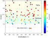 |
Fig. 1 Distribution of the 80 retrograde asteroids. The inclinations and logarithm of the semimajor axes are presented, and the color of each filled circle denotes the value of its eccentricity. An object in the green or yellow region is regarded as a centauror a TNO, respectively. |
For each planet: number of candidates of the 80 retrograde asteroids that lie within the resonant neighborhood (ap∕q − 0.5 au < a < ap∕q + 0.5 au) and number of resonant configurations that these candidates could be trapped in with the corresponding planet.
4 Results of numerical integrations
4.1 Survey of minor bodies in RMMRs
We present the numerical statistical results of the asteroids in RMMRs with planets in Table A.1. All asteroids that are trapped in RMMRs with planets during our integrations are listed. An asteroid was identified as a resonant object if the oscillation of the resonant arguments was found among its ten clones. As listed in Table A.1, 38 asteroids were found to be trapped in 50 RMMRs because some asteroids such as 2008 SO218 evolve in several RMMRs with different planets. In general, it is common to be temporarily captured in resonance for retrograde objects because their orbits are highly eccentric. The retrograde resonant configurations that are identified for the first time here are denoted by an asterisk in Table A.1, and most of them (34/50) are introduced here for the first time. Twenty-eight of these 34 newly introduced retrograde resonant configurations, considering the uncertainty and typical chaoticity of the orbits, are potential candidates for resonant captures. Fifteen asteroids of them are currently in RMMRs, while 30 asteroids will be captured in 35 RMMRs during our integration. These results suggest that the RMMRs with planets are common in retrograde asteroids, and RMMRs could play a crucial role in the origins and evolutions of the retrograde bodies.
As listed in Table A.1, to evaluate the stability of a RMMR, we present the number of resonant clones n, and the highest proportion of time f the clones remain trapped in this resonance relative to the whole integration time-span. For a resonant asteroid, we define its resonant status S as
 (3)
(3)
In our case, the resonant status S is on a scale of 0–10, where the larger S means better and more stable RMMRs. The resonant states S of all the RMMRs are listed in Table A.1, and objects are ordered by their resonant status. Considering the uncertainties of the nominal orbit determination, an RMMR is more reliable and meaningful when its resonant status S is larger than three. Figure 2 depicts the resonant status of all the retrograde resonant asteroids, where 21 objects with the better resonant condition (S > 3) are marked. Asteroids 2015 BZ509, 2000 DG8, and 2011 KT19 have the best resonant situations with S = 10.
Morais & Namouni (2017) identified the first TNO 2011 KT19, nicknamed Niku, which is currently in 7/−9 polar resonance with Neptune. The authors suggested that objects in polar resonances are better protected from disruptive close encounters with planets. de la Fuente Marcos & de la Fuente Marcos (2014) confirmed that two large retrograde Centaurs, 2008 YB3 and 2011 MM4, are trapped in polar resonances with Jovian planets. As listed in Table A.1, 12 asteroids (90° < i ≤ 110°), including 8 Centaurs and 4 TNOs, are currently or will be captured in retrograde polar resonances with Jovian planets. They are 2012 YO6, 2016 TK2, 2005 TJ50, 2008 YB3, 2017 NM2, 2011 SP25, 2011 MM4, 2016 FH13, 2017 UX51, 2016 PN66, 2011 KT19, and 2008 KV42. Some typical polar resonant configurations are shown in Fig. 3. Centaur 2005 TJ50 is the first near-polar asteroid that might currently be in retrograde co-orbital resonance with Saturn. This retrograde resonant episode will end about 20 000 yr later through close encounters with Jupiter. Before and after the 1/−1 resonance with Saturn, it may switch to the 3/−7 polar resonance with Jupiter through close encounters with Saturn. As shown in Fig. 4, 2016 FH13 is the first identified centaur that might be trapped in polar resonance with Uranus, and it will likely be captured in 9/−13 polar resonance with Uranus after close encounters with this planet. However, considering the poor resonant status of 2005 TJ50 and 2016 FH13, more accurate observations and numerical simulations are needed to confirm these results. Moreover, despite the slow precession of the argument of pericenter ω in Fig. 4, we confirmed that 2016 FH13 is not in secular resonance by longer integrations.
Two specific examples are presented to further illustrate the retrograde resonant configurations we identified. First, we focus on centaur 2000 DG8 with the best resonant status, which was discovered on 25 February 2000. This is the first time that 2000 DG8 is identified to currently be in RMMR with Jupiter. As shown in Fig. 5, it has been trapped in 1/− 3 RMMRs with Jupiter at least 10 000 yr and maintains this resonant state throughout our simulation. Other clones of 2000 DG8 also behave similarly. Compared with other normal centaurs, the resonant configuration protects it from frequent close encounters with planets.
Resonance capture plays a vital role in the dynamical evolutions of the minor bodies (Jewitt 2005). Namouni & Morais (2015, 2017, 2018b) studied the resonance capture for arbitrary inclinations, and they hypothesized that retrograde objects are more easily captured in resonance than prograde ones. Recently, Fernández et al. (2018) studied the dynamical evolution including resonance capture of centaurs with perihelia in the Jupiter–Saturn zone. In our simulations, we find that 30 retrograde asteroids will be captured in 35 RMMRs with planets. As shown in Fig. 6, the centaur 2016 LS is currently trapped in 1/− 4 resonance with Jupiter. However, after close encounters with Saturn in around 80 000 yr, it will be captured in 3/− 5 resonance with Saturn. Similarly with 2016 FH13, longer integrations have confirmed that 2016 LS is not in secular resonance. Our results can provide many candidates for the research of retrograde resonant configurations and resonance captures.
We stress the absence of asymmetric librations in retrograde 1/n resonances in Table A.1. It is possible that they do not appear with our definition of critical angle. We will study asymmetric librations in RMMRs further in our future work.
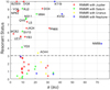 |
Fig. 2 Resonant status S of the asteroids trapped in RMMR with planets (Jupiter in red, Satur in green, Uranus in yellow, and Neptune in blue). Objects whose resonant status is better than 3 are marked. |
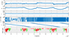 |
Fig. 3 Dynamical evolution of one clone of 2005 TJ50 from −10 000 to 100 000 yr. From top to lower panels: semimajor axis a; eccentricity e; inclination i; 1/− 1 (k = 0) resonant angle with Saturn; argument of pericenter ω; close encounters with giant planets within three corresponding Hill radii, Jupiter (red plus), Saturn (green square), Uranus (purple cross), and Neptune (blue point). |
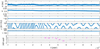 |
Fig. 4 Same as Fig. 3, but for one clone of 2016 FH13. The resonant argument is 9/− 13 (k = 5) with Uranus. |
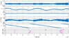 |
Fig. 5 Same as Fig. 3, but for one clone of 2000 DG8. The resonant argument is 1/− 3 (k = 0) with Jupiter. |
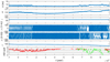 |
Fig. 6 Same as Fig. 3, but for one clone of 2016 LS. The two resonant arguments are 1/− 4 (k = 1) with Jupiter and 3/−5 (k = 2) with Saturn, respectively. |
4.2 Dynamical lifetimes of retrograde asteroids
de la Fuente Marcos & de la Fuente Marcos (2014) analyzed the dynamical evolutions of the 3 large retrograde centaurs (2008 YB3, 2011 MM4, and 2013 LU28). Kankiewicz & Włodarczyk (2017, 2018) studied the dynamical lifetimes of the 25 selected retrograde asteroids. They found that retrograde asteroids are generally unstable, and most of the retrograde asteroids have short life spans (<1 Myr). Of the 25 retrograde asteroids they studied, only three (336756 (2010 NV1), 2011MM4, and 2008 KV42) survived longer than 10 Myr.
In order to estimate dynamical lifetimes of all retrograde asteroids in the solar system, we extended our integration time to 100 Myr. In our numerical simulations, retrograde asteroids are generally unstable and usually ejected from our solar system. The median dynamical lifetimes of ten clones for each retrograde asteroid are depicted in Fig. 7, and most of the retrograde asteroids survived no more than a few million years. Ten retrograde asteroids have median dynamical lifetimes longer than 10 Myr, including 2014 AT28, 2017 NM2, 2011 MM4, 2016 FH13, 2017 QO33, 2011 KT19, 2008 KV42, 2016 NM56, 2017 KZ31, and 2010 NV1. In general, due to the protection of the resonances, eight objects are trapped in RMMRs with planets. 2011 KT19 and 2008 KV42 have the most stable retrograde orbits, and all of their clones are survived the 100 Myr integrations.
The long-term stable dynamics of the two TNOs 2011 KT19 and 2008 KV42 may be due to their particular orbits. As listed in Table 2, they are the only two retrograde TNOs with median eccentricities in the range of 0.3 ~0.5, and their minimum orbit intersection distances (MOIDs) with the giant planets are at least larger than six Hill radii. Moreover, the polar orbits and resonant configurations prevent them from close encounters with planets. Furthermore, we extended the time of our simulations to − 1 Gyr for 100 clones of 2008 KV42 and 2011 KT19 to study their long-time evolutions. Most of the clones survived over the − 1 Gyr integrations.Figure 8 depicts the dynamical evolutions of one clone of 2008 KV42. We find that it was captured in 8/− 13 RMMR with Neptune around −20 Myr after close encounters with Neptune. In general, 2011 KT19 and 2008 KV42 may have the longest dynamical lifetimes of the discovered retrograde asteroids. Studying their orbital and physical characteristics may be helpful for us to understand the origin of the solar system.
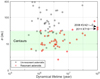 |
Fig. 7 Median dynamical lifetimes of the ten clones for each retrograde asteroid in the 100 Myr numerical simulations. Red filled dots present the objects that are trapped in RMMR, while gray dots denote the asteroids that are not involved with RMMR. An object in the green region is regarded as a centaur. |
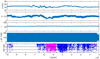 |
Fig. 8 Dynamical evolution of one clone of 2008 KV42 from −1 Gyr to the present day. The basic meaning of this figure is the same as Fig. 3. The resonant argument is 8/− 13 (k = 6) with Neptune. |
4.3 Production of retrograde centaurs
Di Sisto & Brunini (2007) performed a numerical integration of real and synthetic scattered diska (SDOs) to study the origin and distribution of the centaur population. Fernández et al. (2018) numerically studied the dynamical evolution of active and inactive centaurs and analyzed their end states. There are some remarkable features in the retrograde centaurs. First, as shown in Fig. 1, more than half of the discovered retrograde asteroids are centaurs. Centaurs have the highest retrograde fraction of all the dynamical groups or asteroid families (de la Fuente Marcos & de la Fuente Marcos 2014). Second, considering the frequent close encounters with giant planets, the dynamical lifetimes of centaurs are usually far shorter than the age of the solar system (Dones et al. 1996; Levison & Duncan 1997; Tiscareno & Malhotra 2003; Horner et al. 2004; Bailey & Malhotra 2009). As shown in Fig. 7, the dynamical lifetimes of most retrograde centaurs are no longer than a few million years. Moreover, the RMMRs are very common in the retrograde centaurs. As listed in Table A.1, 30 resonant centaurs are among the 45 retrograde centaurs discovered so far. Figure 7 shows that the vast majority of resonant retrograde asteroids are centaurs. Last but not least, Gallardo (2006) presented some asteroids in MMRs with Venus, Earth, and Mars. However, no asteroid trapped in RMMR with the terrestrial planets is discovered in our simulations. Most of the retrograde resonant configurations we identified are involved with Jupiter (55.1%) and Saturn (26.5%).
It is believed that prograde orbits can flip to retrograde states because of the EKM of a Jupiter-sized planet (Lithwick & Naoz 2011; Naoz 2016). Greenstreet et al. (2012) suggested that the EKM of Jupiter can produce retrograde near-Earth asteroids such as 2009 HC82, and most of the test particles are near the 3/1 resonance with Jupiter at the instant when they flip to the retrograde state. Zanardi et al. (2017) and Naoz et al. (2017) suggested that orbits of the outer test particles can also flip from prograde to retrograde or vice versa in the presence of an inner eccentric planet. They discussed the production of debris disk particles by an eccentric Jupiter-mass planet. In our long-term simulations, the orbits of 12 centaurs can flip to prograde state and back again. They are 2007 VW266, 2005 NP82, 2012 YO6, 2014 JJ57, 2016 TP93, 2016 TK2, 2005 TJ50, 2017 SV13, 2016 VY17, 2008 YB3, 2013 NS11, and 2014 PP69. Interestingly, nine centaurs are currently or will be captured in RMMRs, as listed in Table A.1; see, for example, the evolution of centaurs 2013 NS11 (a) and 2016 VY17 (b), depicted in Fig. 9. Centaur 2016 VY17 is trapped in 1/−4 resonance with Jupiter at the moment it flipped. The highest and lowest inclinations during the numerical simulations are shown in Fig. 10. These flippings may be one cause of the existence of retrograde centaurs. This possible production mechanism might also help us to understand the clustering phenomenon of retrograde asteroids in centaurs. However, the common resonant phenomena in retrograde objects may occur just because of their generally high eccentricities. We will study the relationship between the flipping mechanism and RMMRs in centaurs in our future work.
Nominal orbital elements at JED2458600.5 of 2008 KV42 and 2011 KT19.
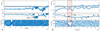 |
Fig. 9 Examples of centaurs, 2013 NS11 (a) and 2016 VY17 (b), that can flip from retrograde to prograde and back again. The resonant arguments are 2/− 3 (k = 0) with Saturn and 1/−4 (k = 0) with Jupiter, respectively. |
5 Conclusions
We have presented the first systematic study of potential asteroids in RMMRs. We did not find asteroids trapped in RMMRs with terrestrial planets, and the majority of RMMRs are involved with Jupiter (55.1%) and Saturn (26.5%). In total, 38 asteroids are identified trapped in 50 RMMRs with giant planets. Fifteen of these asteroids are currently in RMMRs, while 30 asteroids will be captured in 35 RMMRs in future. As shown in Figs. 5 and 6, examples for each case are given to further illustrate their dynamics. We defined the resonant status S to evaluate the stability and condition of a RMMR. Considering the uncertainties of the orbit determination, RMMRs with the resonant status S >3 are more reliable and meaningful. The resonant status S of all the RMMRs is listed in Table A.1 and depicted in Fig. 2.
Our results provide many candidates for research about the retrograde resonant dynamics and captures. Some unusual resonant configurations are found. Twelve retrograde asteroids, including eight centaurs and four TNOs, are identified in polar resonances. For example, 2005 TJ50 may be the first candidate to be currently in retrograde polar co-orbital resonance with a planet, while 2016 FH13 may be the first near-polar centaur that will likely be captured in RMMR with Uranus. Considering the uncertainties of their orbit determination, better observations and more numerical experiments are needed to confirm these results.
We extended the time of our integrations to 100 Myr to study the dynamical lifetimes of all the retrograde asteroids. The majority of retrograde asteroids have short dynamical lifetimes, and they will be quickly ejected from the solar system. As shown in Fig. 7, ten retrograde objects survived longer than 10 Myr, and eight of them are trapped in RMMRs. Numerical integrations confirm that the near-polar TNOs 2011 KT19 and 2008 KV42 could be the retrograde asteroids with the longest dynamical lifetimes. Their particular orbits (near-polar and median eccentricities) and resonant configurations prevent them from close encounters with planets. The integration time was extended to −1 Gyr for 100 clones of 2008 KV42 and 2011 KT19, and most of their clones have survived over 1 Gyr.
The origin of the retrograde objects is always a hot topic in the planetary research, but there are no consistent conclusions so far. As shown in Fig. 9, in our long-term simulations, 12 centaurs can flip to prograde state and back again, and most of them (9 out of 12) are currently or will be captured in RMMRs. For example, centaur 2016 VY17 is trapped in 1/− 4 resonance with Jupiter at the moment it flipped. The highest and lowest inclinations of these 12 centaurs are also depicted in Fig. 10. This flipping mechanism may be one reason for the existence of retrograde centaurs. We will study this possible production mechanism of retrograde centaurs further in our future work.
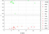 |
Fig. 10 Maximum (in green) and minimum (in red) inclinations of the 12 flipped centaurs during the long-term simulations. Their corresponding semimajor axes are given by the x-axis. |
Acknowledgements
This work was supported by the National Natural Science Foundation of China (Grant No.11772167).
Appendix A Additional table
Asteroids in RMMRs with planets.
References
- Bailey, B. L., & Malhotra, R. 2009, Icarus, 203, 155 [NASA ADS] [CrossRef] [Google Scholar]
- Batygin, K., & Brown, M. E. 2016, ApJ, 833, L3 [NASA ADS] [CrossRef] [Google Scholar]
- Beaugé, C. 1994, Celest. Mech. Dyn. Astron., 60, 225 [NASA ADS] [CrossRef] [Google Scholar]
- Beauge, C., Ferraz-Mello, S., & Michtchenko, T. A. 2003, ApJ, 593, 1124 [Google Scholar]
- Brasser, R., Schwamb, M. E., Lykawka, P. S., & Gomes, R. S. 2012, MNRAS, 420, 3396 [NASA ADS] [CrossRef] [Google Scholar]
- Chambers, J. E. 1999, MNRAS, 304, 793 [NASA ADS] [CrossRef] [MathSciNet] [Google Scholar]
- Chen, Y.-T., Lin, H. W., Holman, M. J., et al. 2016, ApJ, 827, L24 [NASA ADS] [CrossRef] [Google Scholar]
- de la Fuente Marcos, C., & de la Fuente Marcos, R. 2014, Astrophys. Space Sci., 352, 409 [NASA ADS] [CrossRef] [Google Scholar]
- Di Sisto, R. P., & Brunini, A. 2007, Icarus, 190, 224 [NASA ADS] [CrossRef] [EDP Sciences] [Google Scholar]
- Dones, L., Levison, H. F., & Duncan, M. 1996, in Completing the Inventory of the Solar System, eds. T. Rettig, & J. M. Hahn, ASP Conf. Ser., 107, 233 [NASA ADS] [Google Scholar]
- Fernández, J. A., Helal, M., & Gallardo, T. 2018, Planet. Space Sci., 158, 6 [NASA ADS] [CrossRef] [Google Scholar]
- Ferraz-Mello, S., Michtchenko, T. A., & Beaugé, C. 2006, MNRAS, 365, 1160 [NASA ADS] [CrossRef] [Google Scholar]
- Gallardo, T. 2006, Icarus, 184, 29 [Google Scholar]
- Gallardo, T. 2014, Icarus, 231, 273 [NASA ADS] [CrossRef] [Google Scholar]
- Gallardo, T. 2019a, Icarus, 317, 121 [NASA ADS] [CrossRef] [Google Scholar]
- Gallardo, T. 2019b, MNRAS, 487, 1709 [NASA ADS] [CrossRef] [Google Scholar]
- Greenstreet, S., Gladman, B., Ngo, H., Granvik, M., & Larson, S. 2012, ApJ, 749, L39 [NASA ADS] [CrossRef] [Google Scholar]
- Horner, J., Evans, N. W., & Bailey, M. E. 2004, MNRAS, 354, 798 [NASA ADS] [CrossRef] [Google Scholar]
- Huang, Y., Li, M., Li, J., & Gong, S. 2018a, AJ, 155, 262 [NASA ADS] [CrossRef] [Google Scholar]
- Huang, Y., Li, M., Li, J., & Gong, S. 2018b, MNRAS, 481, 5401 [NASA ADS] [CrossRef] [Google Scholar]
- Jewitt, D. 2005, AJ, 129, 530 [NASA ADS] [CrossRef] [Google Scholar]
- Kankiewicz, P., & Włodarczyk, I. 2017, MNRAS, 468, 4143 [NASA ADS] [CrossRef] [Google Scholar]
- Kankiewicz, P., & Włodarczyk, I. 2018, Planet. Space Sci., 154, 72 [NASA ADS] [CrossRef] [Google Scholar]
- Levison, H. F., & Duncan, M. J. 1997, Icarus, 127, 13 [Google Scholar]
- Li, M., Huang, Y., & Gong, S. 2018, A&A, 617, A114 [NASA ADS] [CrossRef] [EDP Sciences] [Google Scholar]
- Li, M., Huang, Y., & Gong, S. 2019, Astrophys. Space Sci., 364, 78 [NASA ADS] [CrossRef] [Google Scholar]
- Lithwick, Y., & Naoz, S. 2011, ApJ, 742, 94 [NASA ADS] [CrossRef] [Google Scholar]
- Morais, M. H. M., & Namouni, F. 2013a, MNRAS, 436, L30 [NASA ADS] [CrossRef] [Google Scholar]
- Morais, M. H. M., & Namouni, F. 2013b, Celest. Mech. Dyn. Astron., 117, 405 [NASA ADS] [CrossRef] [Google Scholar]
- Morais, M. H. M., & Namouni, F. 2016, Celest. Mech. Dyn. Astron., 125, 91 [NASA ADS] [CrossRef] [Google Scholar]
- Morais, M. H. M., & Namouni, F. 2017, MNRAS, 472, L1 [NASA ADS] [CrossRef] [Google Scholar]
- Morbidelli, A. 2002, Modern Celestial Mechanics: Aspects of Solar System Dynamics (London: Taylor & Francis) [Google Scholar]
- Morbidelli, A., Zappala, V., Moons, M., Cellino, A., & Gonczi, R. 1995, Icarus, 118, 132 [NASA ADS] [CrossRef] [Google Scholar]
- Murray, C. D., & Dermott, S. F. 1999, Solar System Dynamics (Cambridge: Cambridge University Press) [Google Scholar]
- Namouni, F., & Morais, M. H. M. 2015, MNRAS, 446, 1998 [NASA ADS] [CrossRef] [Google Scholar]
- Namouni, F., & Morais, M. H. M. 2017, MNRAS, 467, 2673 [NASA ADS] [CrossRef] [Google Scholar]
- Namouni, F., & Morais, M. H. M. 2018a, MNRAS, 477, L117 [NASA ADS] [CrossRef] [Google Scholar]
- Namouni, F., & Morais, H. 2018b, Comput. Appl. Math., 37, 65 [CrossRef] [Google Scholar]
- Naoz, S. 2016, ARA&A, 54, 441 [Google Scholar]
- Naoz, S., Li, G., Zanardi, M., de Elía, G. C., & Di Sisto, R. P. 2017, AJ, 154, 18 [NASA ADS] [CrossRef] [Google Scholar]
- Narita, N., Sato, B., Hirano, T., & Tamura, M. 2009, PASJ, 61, L35 [NASA ADS] [Google Scholar]
- Nesvorný, D., Ferraz-Mello, S., Holman, M., & Morbidelli, A. 2002, Regular and Chaotic Dynamics in the Mean-Motion Resonances: Implications for the Structure and Evolution of the Asteroid Belt, eds. W. F. Bottke, Jr. A. Cellino, P. Paolicchi, & R. P. Binzel, 379 [Google Scholar]
- Smirnov, E. A., Dovgalev, I. S., & Popova, E. A. 2018, Icarus, 304, 24 [NASA ADS] [CrossRef] [Google Scholar]
- Tiscareno, M. S., & Malhotra, R. 2003, AJ, 126, 3122 [NASA ADS] [CrossRef] [Google Scholar]
- Triaud, A. H. M. J., Collier Cameron, A., Queloz, D., et al. 2010, A&A, 524, A25 [NASA ADS] [CrossRef] [EDP Sciences] [Google Scholar]
- Voyatzis, G., Tsiganis, K., & Antoniadou, K. I. 2018, Celest. Mech. Dyn. Astron., 130, 29 [NASA ADS] [CrossRef] [Google Scholar]
- Wiegert, P., Connors, M., & Veillet, C. 2017, Nature, 543, 687 [NASA ADS] [CrossRef] [Google Scholar]
- Winn, J. N., Johnson, J. A., Albrecht, S., et al. 2009, ApJ, 703, L99 [NASA ADS] [CrossRef] [Google Scholar]
- Zanardi, M., de Elía, G. C., Di Sisto, R. P., et al. 2017, A&A, 605, A64 [NASA ADS] [CrossRef] [EDP Sciences] [Google Scholar]
Taken from the website of the JPL Small-Body Database Search Engine; https://ssd.jpl.nasa.gov, retrieved on 20 April 2019.
All Tables
For each planet: number of candidates of the 80 retrograde asteroids that lie within the resonant neighborhood (ap∕q − 0.5 au < a < ap∕q + 0.5 au) and number of resonant configurations that these candidates could be trapped in with the corresponding planet.
All Figures
|
Fig. 1 Distribution of the 80 retrograde asteroids. The inclinations and logarithm of the semimajor axes are presented, and the color of each filled circle denotes the value of its eccentricity. An object in the green or yellow region is regarded as a centauror a TNO, respectively. |
| In the text | |
|
Fig. 2 Resonant status S of the asteroids trapped in RMMR with planets (Jupiter in red, Satur in green, Uranus in yellow, and Neptune in blue). Objects whose resonant status is better than 3 are marked. |
| In the text | |
|
Fig. 3 Dynamical evolution of one clone of 2005 TJ50 from −10 000 to 100 000 yr. From top to lower panels: semimajor axis a; eccentricity e; inclination i; 1/− 1 (k = 0) resonant angle with Saturn; argument of pericenter ω; close encounters with giant planets within three corresponding Hill radii, Jupiter (red plus), Saturn (green square), Uranus (purple cross), and Neptune (blue point). |
| In the text | |
|
Fig. 4 Same as Fig. 3, but for one clone of 2016 FH13. The resonant argument is 9/− 13 (k = 5) with Uranus. |
| In the text | |
|
Fig. 5 Same as Fig. 3, but for one clone of 2000 DG8. The resonant argument is 1/− 3 (k = 0) with Jupiter. |
| In the text | |
|
Fig. 6 Same as Fig. 3, but for one clone of 2016 LS. The two resonant arguments are 1/− 4 (k = 1) with Jupiter and 3/−5 (k = 2) with Saturn, respectively. |
| In the text | |
|
Fig. 7 Median dynamical lifetimes of the ten clones for each retrograde asteroid in the 100 Myr numerical simulations. Red filled dots present the objects that are trapped in RMMR, while gray dots denote the asteroids that are not involved with RMMR. An object in the green region is regarded as a centaur. |
| In the text | |
|
Fig. 8 Dynamical evolution of one clone of 2008 KV42 from −1 Gyr to the present day. The basic meaning of this figure is the same as Fig. 3. The resonant argument is 8/− 13 (k = 6) with Neptune. |
| In the text | |
|
Fig. 9 Examples of centaurs, 2013 NS11 (a) and 2016 VY17 (b), that can flip from retrograde to prograde and back again. The resonant arguments are 2/− 3 (k = 0) with Saturn and 1/−4 (k = 0) with Jupiter, respectively. |
| In the text | |
|
Fig. 10 Maximum (in green) and minimum (in red) inclinations of the 12 flipped centaurs during the long-term simulations. Their corresponding semimajor axes are given by the x-axis. |
| In the text | |
Current usage metrics show cumulative count of Article Views (full-text article views including HTML views, PDF and ePub downloads, according to the available data) and Abstracts Views on Vision4Press platform.
Data correspond to usage on the plateform after 2015. The current usage metrics is available 48-96 hours after online publication and is updated daily on week days.
Initial download of the metrics may take a while.