| Issue |
A&A
Volume 630, October 2019
Rosetta mission full comet phase results
|
|
|---|---|---|
| Article Number | A17 | |
| Number of page(s) | 10 | |
| Section | Planets and planetary systems | |
| DOI | https://doi.org/10.1051/0004-6361/201732094 | |
| Published online | 20 September 2019 | |
Seasonal variations in source regions of the dust jets on comet 67P/Churyumov-Gerasimenko
1
Graduate Institute of Space Sciences, National Central University,
Taoyuan City 32001,
Taiwan
e-mail: ianlai@g.ncu.edu.tw
2
Institute of Astronomy, National Central University,
Taoyuan City 32001, Taiwan
3
Space Science Institute, Macau University of Science and Technology,
Macau, PR China
4
Department of Earth Science, National Central University,
Taoyuan City 32001, Taiwan
5
German Aerospace Center (DLR), Institute of Planetary Research,
Rutherfordstraeβ 2,
12489 Berlin, Germany
6
Max-Planck-Institut für Sonnensystemforschung,
Justus-von-Liebig-Weg,
3 37077 Göttingen, Germany
7
Department of Physics and Astronomy, University of Padova,
Vicolo dell’Osservatorio 3,
35122 Padova, Italy
8
LAM (Laboratoire d’Astrophysique de Marseille), CNRS, Aix Marseille Université, UMR 7326,
38 rue Frédéric Joliot-Curie,
13388 Marseille, France
9
Centro de Astrobiologia, CSIC-INTA,
28850 Torrejon de Ardoz,
Madrid, Spain
10
International Space Science Institute,
Hallerstraβe 6,
3012 Bern, Switzerland
11
Scientific Support Office, European Space Research and Technology Centre/ESA,
Keplerlaan 1,
Postbus 299,
2201 AZ Noordwijk ZH, The Netherlands
12
Department of Physics and Astronomy, Uppsala University,
Box 516,
75120 Uppsala, Sweden
13
PAS Space Research Center,
Bartycka 18A,
00716 Warszawa, Poland
14
Institut für Geophysik und extraterrestrische Physik (IGEP), Technische Universität Braunschweig,
Mendelssohnstr. 3,
38106 Braunschweig, Germany
15
LESIA-Observatoire de Paris, CNRS, Université Pierre et Marie Curie, Université Paris Diderot,
5 place J. Janssen,
92195 Meudon, France
16
CNR-IFN UOS Padova LUXOR,
Via Trasea, 7,
35131 Padova, Italy
17
Center of Studies and Activities for Space G. Colombo, CISAS, “G. Colombo”, University of Padova,
Padova, Italy
18
INAF, Osservatorio Astronomico di Padova,
Vicolo dell’Osservatorio 5,
35122 Padova, Italy
19
Department of Physics and Astronomy, Uppsala University,
Box 516,
75120 Uppsala, Sweden
20
Department of Industrial Engineering, University of Padova,
Via Venezia 1,
35131 Padova, Italy
21
University of Trento,
Via Mesiano 77,
38100 Trento, Italy
22
INAF – Osservatorio Astronomico,
Via Tiepolo 11,
34014 Trieste, Italy
23
Instituto de Astrofísica de Andalucía (CSIC),
Glorieta de la Astronomìa,
18008 Granada, Spain
24
Operations Department, European Space Astronomy Centre/ESA,
PO Box 78,
28691 Villanueva de la Canada,
Madrid, Spain
25
Department of Information Engineering, University of Padova,
Via Gradenigo 6/B,
35131 Padova, Italy
26
Physikalisches Institut der Universität Bern,
Sidlerstr. 5,
3012 Bern, Switzerland
27
Department of Physics, Auburn University,
Auburn,
AL 36849, USA
Received:
12
October
2017
Accepted:
5
October
2018
Aims. We investigate the surface distribution of the source regions of dust jets on comet 67P/Churyumov-Gerasimenko as a function of time.
Methods. The dust jet source regions were traced by the comprehensive imaging data set provided by the OSIRIS scientific camera.
Results. We show in detail how the projected footpoints of the dust jets and hence the outgassing zone would move in consonance with the sunlit belt. Furthermore, a number of source regions characterized by repeated jet activity might be the result of local topographical variations or compositional heterogeneities.
Conclusions. The spatial and temporal variations in source regions of the dust jets are influenced significantly by the seasonal effect. The strong dependence on the solar zenith angle and local time could be related to the gas sublimation process driven by solar insolation on a surface layer of low thermal inertia.
Key words: comets: individual: 67P/Churyumov-Gerasimenko
© ESO 2019
1 Introduction
The detailed imaging observations of comet 67P/Churyumov-Gerasimenko (67P) showed that its outgassing behavior was controlled by its bi-lobate structure of the cometary nucleus and its obliquity of 52 degrees (Sierks et al. 2015; Keller et al. 2015). During the early part of the inbound orbit, only the northern hemisphere was illuminated. The subsolar point gradually shifted from north to south until the equinox on May 10, 2015. Since then, the southern hemisphere became more and more active. The maximum gas production rate of Q ~ 3.5 × 1028 H2O s−1 occurred 18–22 days after perihelion (Hansen et al. 2016; Marshall et al. 2017). Even though the time interval (~8 months) of the southern surface heating is shorter than the orbital period, the corresponding sublimation process has a great effect on the evolution of the geomorphology of the comet itself. The accompanying emission and transport of dust grains have been investigated in several studies (Sierks et al. 2015; Thomas et al. 2015; Keller et al. 2015; Lai et al. 2016; Hu et al. 2017). That is, the reimpact of the dust grains ejected from the southern hemisphere during the perihelion passage could lead to erosion of the southern surface material while depositing dust layers on the northern side. This could be the physical cause of the dramatic dichotomy of the smooth feature of the Hapi region and the very rugged terrain of the antipodal Sobek region (Thomas et al. 2015; Lai et al. 2016; Keller et al. 2017). This also means that the time evolution of the dust coma structure as traced by the total brightness and the fine structures could provide important information about this key process. Since the start of the monitoring phase in August 2014, the formation and source regions of collimated dust jets and their time evolution were first documented by Lin et al. (2015) and Lara et al. (2015). During this period, the radial dust jets were most prominent in the northern part of the coma, and their footpoints could be traced to the center of the Hapi region and two sides of the surrounding cliffs (Sierks et al. 2015; Lin et al. 2015; Lara et al. 2015).
The area of Hapi jet activity coincided with the smooth terrains that are characterized by bluer spectral slopes (Fornasier et al. 2015; Oklay et al. 2015). The recurrent dust features probably belong to the Type 1 jets that are produced by water-ice sublimation, as defined by Belton (2010). These coma jets appeared to be driven by solar illumination, indicated by the radiative heating effect of water-ice-rich material situated at a depth shallower than one thermal skin (~1 cm) from the dust-covered surface.
According to Belton (2010), there are two other types of jets: the Type 2 jets that represent filamentary structure emanating from localized topographical spots such as the edge of active pits or cliffs (Vincent et al. 2015, 2016a), and the Type 3 outbursts that are created by explosive events as documented by Knollenberg et al. (2016), Vincent et al. (2016b), Pajola et al. (2017), and Lin et al. (2017). Vincent et al. (2016b) and Lin et al. (2017) showed that unlike the faint Type 1 jets with multiple appearances in succeeding rotations, the bright Type 3 transient events that last just a few minutes did not repeat themselves. Their source locations can be found in the vicinity of steep cliffs. That the outbursts occurred most often at either early morning or afternoon indicates that they could have been triggered by thermal stress. Alternatively, the sudden opening of a fracture or crack, also because of thermal stress, could also lead to a violent sublimation of the super-volatile ices buried in the deep interior according to Skorov et al. (2016).
In spite of their very different source mechanisms and occurrence times, these three types of jets might be associated with each other. For example, the Type 1 jet activity might be found at water-ice exposures near the foot of collapsed cliffs (Vincent et al. 2015), and, of course, the icy dust grains ejected in outbursts could be returned to the nucleus surface in the form of backfall, thus providing the source material for the recurrent jets (Thomas et al. 2015; Lai et al. 2016; Keller et al. 2017).
To return to the main topic of the recurrent Type 1 jets, the Optical, Spectroscopic, and Infrared Remote Imaging System (OSIRIS) cameras (Keller et al. 2007) provided us with thousands of images that can be used to investigate the dust jets of 67P. As illustrated in Fig. 1, the jet features gradually changed their strengths and configuration as 67P approached perihelion. Schmitt et al. (2017) examined the occurrences of jet features from 2014 December to 2015 October and mapped their source locations on the nucleus surface as a function of time. Similar results, that the sources followed the subsolar latitude, were reported earlier (Ip et al. 2016). The purpose of this work is therefore to present the full set of spatial distributions of the jet sources for the whole Rosetta mission between July 2014 and March 2016, before the Rosetta spacecraft moved too close to the comet to provide global coverage of the dust coma. In Sect. 2, we briefly describe the numerical method of ray-tracing the footpoints of linear structures in the dust coma. In Sect. 3, we show the locations of the jet sources on the cometary surface from month to month, complemented by statistical studies of their occurrence frequencies, which might be related to the gas production rates. In Sect. 4, we investigate the dependences of the jet activity on the local time and the solar zenith angle (SZA). The SZA values are obtained by using the shape model to account for the highly variable topography of the comet nucleus. Special attention is paid to the possible correlation of source regions with repeated jet occurrence and a number of geomorphological features in Sect. 4. A summary and discussion are given in Sect. 5.
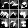 |
Fig. 1 OSIRIS image of jet features of comet 67P from 2014 to 2016. The sunlit side shifted from the northern to the southern hemisphere after the equinox in August, 2015. The dust jets are mostly cone-like structures. The cone angle of the wide jets could be up to 35° and that of the narrow jets about 10°. |
2 Method
As shown inFig. 1, amid the diffuse background of the dust coma, many fine structures can be recognized and appear to be straight and collimated. Furthermore, they are mostly perpendicular to the surface where they first emerge. In the coma images of OSIRIS, the dust sizes should be on the order of 0.1–1 mm according to Rotundi et al. (2015). This estimate is consistent with the model calculation of the curved jets by Lin et al. (2016). A similar property was observed for the jet activity of 9P/Tempel 1 (Farnham et al. 2013). With the assumption that the observed collimated structures are dust streams in the hydrodynamics sense, a ray-tracing technique to connect the narrow dustjets and their footpoints on the nucleus surface similar to the method of Spitale & Porco (2007) for identifying the jetlets of the Enceladus plume can be applied (Farnham et al. 2013; Lin et al. 2015; Vincent et al. 2016a).
As an example, Fig. 2 depicts the procedure of selecting jet structures in the OSIRIS images. Figure 2a is an original image with the brightness distribution in linear scale. The jets are too faint to be recognized. In Fig. 2b, the brightness distribution is in logarithmic scale. Even without stretching the dynamic range of the image, the jet system in the sunwarddirection is now visible. Figs. 2c–e represent images in log scale with the stretching factor (F) varying from 0.8, 0.4, to 0.2, respectively. The stretching factor is the ratio of the maximum value of brightness between the original image and the stretched image. By varying F, five jets were selected through visual inspection, as shown in Fig. 2c. Finally, the normalized brightness distribution in a circle close to the nucleus surface is shown in Fig. 2f to delineate these jets. The jet widths vary, but could be estimated to be on the order of 10°–35° (or 0.4–1.5 km) on average. Since most of the jet features are narrow, the typical value of the error circle of the jet source localization is hence approximately 200 m. This might be considered the radius of the error circle of the jet source localization. The peak brightness of each jet is generally higher than 0.2 in the normalized brightness scale. Even though the actual brightness of the dust coma in different orbital positions would be different, the exposure times of the OSIRIS observationswere adjusted accordingly. This means that most of the jet features would be identified by using F ~ 0.6 in the above procedure.
After finding the angular position of a jet in an OSIRIS image, a jet line outlining the jet feature can be defined. The 2D image plane can then be transformed into the 3D cometary rotating frame using the SPICE toolkit. The jet source is located in the plane containing the jet line and perpendicular to the image plane. As explained in Fig. 3, if the same jet was identified in two sequential images obtained at different viewing angles, the intersection of these two panels containing the two 2D jet lines will determine the 3D structure of the dust jet and its source location. In total, there are 16 816 facets with a typical size of 500 m. The footpoints of the jet lines were charted by using a simplified SHAPS5 shpae model (Jorda et al. 2016).
Figure 3 shows an example of the method. This method has been applied to characterize the jet source regions in the pits by Vincent et al. (2015). As the comet approached perihelion, its outgassing activity increased significantly, and it became difficult to identify the same jet in two images. To overcome this problem, we chose to examine jet structures in consecutive images taken at short time intervals (~ 1–2 h). The source regions of multiple jets can be located in this manner. To reduce uncertainties in the numerical analysis, jet sources occurring on the dark side were not included in the statistical study.
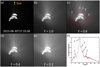 |
Fig. 2 Profile of the narrow dust jets. (a) We extract the brightness data from a red circle on an OSIRIS image. (b) Brightness profile of the dust coma and five identified jet features (Image ID: NAC_2015-08-30T17.33.04.154Z_ID30_1397549005_F22). |
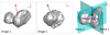 |
Fig. 3 Example of the method with which we identified the jet source regions. The source region is defined by the intersection of two planes that are perpendicular to the camera plane and include the jet line. |
3 Time variability of the jet source regions
Several factors would affect the statistical results of jet counts. The first has to do with the availability of pertinent imaging data at different times. To track the long-term trend from month to month, the limitation through data gaps might not be very critical. Another detrimental factor is that jet features are most clearly visible at the limb. This condition of the viewing geometry might thus lead to an inaccuracy in the statistical survey of the spatial distribution of the jet sources on the nucleus surface. To mitigate this projection bias, we used mostly image sequences covering more than one rotation period. In order to improve the time coverage, two sets of image sequences were used in each month (see Table 1). After March 2016, no clear jet images were available because the distance to the comet nucleus was so short. We used 33 image sequences and 409 images taken between November 12, 2014, and March 23, 2016. A summary of the sequence numbers and observation times can be found in Table 1. We identified3530 candidate jet source regions in these images. The exact locations cannot be precisely determined because of the limitation in image matching/comparison and assessment. As described before, because of the ray-tracing method, the radius of the error circle could be as large as 200 m for the majority of the (narrow) jet features.
Figure 4 shows the jet source locations we identified by the ray-tracing method. In general agreement with the ealier studies of Ip et al. (2016) and Schmitt et al. (2017), our results indicate a gradual migration of the footpoints from the northern pole to the mid-latitudinal regions and then equator-ward between August 2014 and May 2015 (see Fig. 4). After the equinox in May 2015, jets started to pepper the southern part of the comet nucleus as it emerged from darkness. The Hapi jets were turned off in May 2015, and a cluster of jet sources instead appeared in the region between Ma’at and Hatmehit. Figure 4b illustrates that after reaching the peak of the southern summer in August 2015 at perihelion, the jet sources moved equatorially once again until they spread into the northern hemisphere. The higher concentration of jet sources in the Wosret region may be partially caused by the 2D Mercator projection. On the other hand, MIRO measurements indicated that Wosret and its neighboring areas did have higher water production rates in this time interval (Marshall et al. 2017).
Figure 5 is a surface density map of the jet sources produced from all of the collecting data points in Fig. 4. In our computation, a facet is defined to be active if it is within 200 m of a footpoint. The northern part is less active, except for the Hapi region as a whole. Furthermore, a number of localized hot spots in the southern part can be identified, suggesting the possible repetition of dust jet formation. Even though the ratio of the surface density of the so-called hot spots to that of the average value is only on the order of 2–3, it is interesting to examine more closely whether their corresponding surface areas are characterized by special geological features of compositional difference or topographical variation. It should also be noted that this surface density map of the jet sources is biased by the frequency of the relevant observations made at different times and the orientation of the comet nucleus and viewing geometry, among other factors. These points are discussed later.
In Fig. 6, we show a plot of the solar radiation influx integrated over the time interval between November 2014 and March 2016. This heat map matches Fig. 5 well, except for the hot spots, which might be related to surface geomorphological structures. This comparison also indicates that the map of the surface density distribution of the jet source given in Fig. 5 is a reasonable representation of the gas sublimation process as a function of time. When the surface density of the jet source locations in each grid point of the map given in Fig. 5 is divided by the corresponding solar energy flux distribution, we find that the Hapi region with its relatively smooth plain is particularly active in generating dust jets, even though it received only a small amount of solar radiation.
Summary of the OSIRIS image sequences used in the jet source survey.
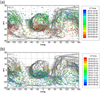 |
Fig. 4 Time variation in locations of the jet source regions (or footpoints) from month to month during the Rosetta close-up observationsin the (a) pre-perihelion period and (b) post-perihelion period. The black triangles show the additional jet sources between August and September 2014 from Lin et al. (2015). The dots represent the footpoint positions of the jet, with an error circle radius of about 200 m for most cases. |
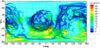 |
Fig. 5 Surface density distribution of the 3530 jet source locations identified in our image analysis and ray-tracing calculation. |
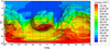 |
Fig. 6 Map of the cumulative solar radiative energy flux distribution on the nucleus surface from November 2014 to March 2016. |
4 Local time and solar zenith angle dependence
Monitoring observations of the outgassing activity of comet 67P by different instruments on Rosetta indicated that the whole surface of this comet could emit gas and dust, and the production rates depended mainly on the sunlit condition and the heliocentric distances. As a result, jet sources typically follow the subsolar latitude, and the area of maximum activity migrates accordingly. This fact was reported in earlier papers, for instance, Kramer et al. (2017) based on ROSINA data. The dependence on subsolar longitude, or local time, is equally interesting as it relates to the thermal inertia of the material and/or the depth at which volatiles are buried. According to Shi et al. (2016), early observations in 2014 show that jet sources switched on and off as soon as they crossed the morning or evening terminator. Conversely, later observations (< 1.8 au) revealed that if the energy input was sufficient, jets could be sustained for at least an hour beyond sunset. The detection of a mini-outburst from the nightside on 12 March 2015 is also noteworthy (Knollenberg et al. 2016). These events indicated that some areas might host volatiles at a greater depth, where thermal variations would occur more slowly, with the maximum temperaturelagging behind the temperature profile at the very top surface.
Tracking every jet over a full rotation is not possible with our dataset, but we can make some global statistical analysis. The SZA can be calculated as the angle between the normal vector of the facet of the jet source footpoint and the sunlit direction. Local noon can be defined for the facet of the dust jet source with a minimum SZA in one rotation period. Figure 7a, for instance, shows the number of observed jets as a function of LT, integrated over the whole mission. Interestingly, we find that the distribution can be approximated with a Gaussian function with a center at LT = 11.84 and a sigma of 3.98 h. This means that at any epoch, about 60% of the jets are produced near local noon (LT = 10–14). If the number of dust jets closely tracks the gas sublimation rate (Z), no time lag between local noon and the peak value of Z indicates extremely low thermal inertia (TI), compatible with measurements (i.e., TI = 50 J m−2 K−1s−1∕2 by MIRO inSchloerb et al. 2015). It also means that the sublimating layer must be within the diurnal thermal skin depth of the surface, as the jet activity seems to respond almost immediately to solar insolation.
Anotherinteresting exercise is to compare the jet occurrence frequency as a function of SZAs. As shown in Fig. 7b, the surface density distribution of the dust jets is indeed very sensitive to SZA. As a rough topography with cliffs and pits will producea wide range of local SZAs within a small region, which would have a strong influence on the gas and dust production rates, these correlatives must be examined in more detail so that their physical mechanisms can be further understood.
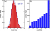 |
Fig. 7 Panel a: local time distribution. Panel b: solar zenith angle distribution of the jet sources. |
5 Surface morphology
According to Fig. 5, a number of relatively higher jet source concentrations can be identified in the southern hemisphere. Figure 8 compares the surface density maps of the jet sources with the OSIRIS images of the three regions that are embedded in Imhotep, Wosret, Sobek, and Bes, respectively. Because of the limitation of our ray-tracing method, only the general areas can be identified. In Fig. 8a, the hot spot of jet activity is located near a cliff in the Imhotep region in the southern hemisphere and is characterized by a smooth terrain filled with boulders (Lee et al. 2016). We detect jet structures from April 2015 to December 2015 in this region.
Figure 8d shows a hot spot in a pit of the Wosret region on the southern hemisphere. This pit may be one of the active pits described by Vincent et al. (2015). In this region, we detect dust jets from May 2015 to October 2015. In Fig. 8g, the hot spot is located in the Sobek region near a series of scarps (Lee et al. 2016) that seem to be located in the vicinity of pits. The active period is from May 2015 to October 2015. In Fig. 8j this hot spot is located near a cliff in the Bes region. This region is covered with fine material and might be related to a bright spot that has been detected by Oklay et al. (2017). The active period is from May 2015 to November 2015.
It is noteworthy that these clusters of jet sources became noticeable mostly just before the equinox in May 2015. Some, such as those in Imhotep, Wosret, and Bes, would continue for several months until the end of year. This means that the physical causes of these dust jets probably have less to do with the sudden change of geological structures, as in the case of the one-time outbursts depicted by Vincent et al. (2016b) and the one on 10 July 2015 that was generated by the collapse of the Aswan cliff (Pajola et al. 2017). It is possible that some fractures or surface cracks of smaller magnitude produced by enhanced thermal stress during the perihelion passage could trigger the observed repetition of dust jet activities. On the other hand, the penetration of the heat wave to the bottoms of some of the dormant pits might reactivate the sublimation process.
Figure 9 shows a projection of the jet source number density distribution in Imhotep and Bes onto the shape model of the comet, oriented to match the viewing geometry of an NAC color-composite image. This illustrates the possible correlation between the two main clusters of activity in Imhotep and the prominent water-ice-enriched areas in the same region, as described in Oklay et al. (2017). These flat areas contain exposed surface material with high volatile material content, which can sublimate away when illuminated. The cliffs surrounding the source terrain focus the gas flow that is released from the ice patches and lead to the jet formation, a process described in Vincent et al. (2016a) for other regions of 67P.
It is interesting to note that almost every cliff on 67P is likely to produce a jet, as long as a gas flow exists near by. The source of the gas flow is typically the boulder talus at the foot of a collapsed cliff. Although the process is similar here, we note that the two cliffs in Imhotep do not show much rubble in their taluses and are considerably brighter than other areas. In addition, the terrain at the foot of the cliffs appears smooth and subdued, and the low spectral slope (typical of water-rich content) has persisted for extended periods (>1 yr, see Oklay et al. 2017). This means that the source of volatiles in these two areas is not simply fresh debris from the collapsing cliffs, but probably local water reservoirs buried just below these areas that constantly feed the jets. This would explain why these areas remain spectrally
distinct for a long time, and why more jets can be generated here than in other regions with similar morphologies.
In a recent paper, Kramer et al. (2017) have also identified localized regions of enhanced activity using gas-monitoring data
from the ROSINA instrument. Although the uncertainty of their source locations is large because the collimation factor of gas flows is lower than that of dust jets, they also found clustering of activity in zones that correspond to our inversion.
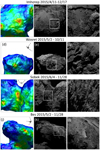 |
Fig. 8 Four regions with higher concentration of dust jet sources according to the shape model and OSIRIS images in increasingly finer spatial scales: the first row shows Imhotep (a–c), the second row Wosret (d–f), the third row shows Sobek (g–i), and fourth row the Bes region (j–l). |
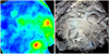 |
Fig. 9 Comparison of the two higher concentration regions in Imhotep and Bes with an NAC color-composite image from Oklay et al. (2017). |
6 Summary and discussion
We have examined the time evolution of the spatial distribution of the dust jet sources on comet 67P from November 2014 to March 2016 based on an analysis of the OSIRIS imaging data. The main results are listed below.
- 1.
Using a ray-tracing method (Spitale & Porco 2007; Farnham et al. 2013; Lin et al. 2015; Vincent et al. 2016a), we identified 3530 collimated jets by visual inspection. We find that the location of the jet source regions is correlated with theseasonal variation of the sunlit latitude of 67P.
- 2.
The angular widths of the cone-shaped jet structures identified in our study vary from about 10° to 35°. For mostof jets that have a narrow with full width of about 10° or smaller, the error circle radius of footpoints or the source locations could be on the order of a few hundred meters.
- 3.
The occurrence frequency of the jet features with their SZA averaged over the footpoints peaks at noon or near zero zenith angle, according to the surface projection on the shape model of the nucleus of 67P.
- 4.
Several regions with enhanced jet activity, in particular in the southern hemisphere, have been identified. When compared with morphological structures on the nucleus surface, these hot spots appear to be associated with pits in Wosret and Sobek, and a cliff in Bes. On the other hand, some jet sources in Imhotep could be connected to localized areas with exposed water ice.
The interpretation of these observational results is based on one main assumption: the dust jet structures are associated with the thermal sublimation of water ice. To some extent, this connection must be true since the latitudinal distribution of the jet sources coincides with the seasonal change of the sunlit zone. The exact physical origin of the narrow dust jets is less certain. Several possibilities have been discussed. The first had to do with the projection effect of a wavy curtain of dust outflow from the nucleus surface. The integrated brightness along the line of sight at certain viewing angles could give the impression of a system of collimated jets (Lin et al. 2015; Shi et al. 2018). Such a phenomenon has also been discussed in the context of the jets in the Enceladus plume (Spitale et al. 2015). The second possibility considers the focusing effect by (concave) topographic structures on the cometary nucleus surface with homogeneous gas and dust emission rates on the sunlit side. This mechanism has been investigated in detail in the case of 67P by Kramer & Noack (2016). Recurrent jet formation is expected in this model. The hot spots in the jet source distributions in Wosret, Sobek, and Bes identified in Fig. 8 might be of this origin. The third effect has to do with the presence of inhomogeneous gas and dust emission rates on the nucleus surface. An example could be the localized regions of enhanced jet activity in Imhotep that overlap the potentially water-ice-rich areas pinpointed by Oklay et al. (2017). Spatial variation of gas or dust emission rates at a small scale could also lead to the pressure-driven collimation effect described previously by Koemle & Ip (1987) in the context of the sunward jets of comet Halley. Finally, Shi et al. (2016) produced evidence that dust jet structures are generated at the boundary of the solar isolation, possibly as a result of water-ice recondensation in the shadowed region (De Sanctis et al. 2015). This means that the observed jet features could have different formation mechanisms because of the irregular topography (i.e., cliffs and pits), complex temporal change in isolation effect, and chemical heterogeneity of the surface (or subsurface) material.
An interesting and somewhat surprising result in our study has to do with the strong zenith angle dependence of the occurrence frequency of the dust jet structures shown in Fig. 7. While this effect is consistent with the thermal sublimation of water ice under a thin dust layer characterized by lower thermal inertia of about 50 MKS according to Schloerb et al. (2015), a great discrepancy exists with the peak gas emission angles of H2O observed by MIRO (Lee et al. 2015) and H2O and CO2 by VIRTIS (Bockelée-Morvan et al. 2016). One possible explanation is that the dust outflow accelerated by the gas drag force is basically determined by the surface gas emission pattern controlled by the solar isolation. That is, the outgassing rate (Zi) at the ith facet can be approximated to be Zi ~ max (a, cos θi), where θi is the local zenith angle and a ~ 0.1 (Biver et al. 2015). On the other hand, the expanding gas outflow could be significantly modified by the large-scale morphology of the nucleus, as demonstrated by DSMC model calculations (Lai et al. 2016; Liao et al. 2018).
Becauseof the constraint that no jets on the nightside would be counted (or identified), this effect would introduce a certain bias in the counting of the jet features. As a test to simulate the SZA dependence that would occur for a uniform distribution of the jet sources over the sunlit surface of 67P, we have produced a Monte Carlo model to introduce a random distribution of dust jets across the illuminated nucleus surface as the comet rotates below the spacecraft (fixed at a certain orbital position). The specific seasonal interval of the simulation was May 2015. The jet structures visible above the limb were counted and registered for statistical analysis. We find that over one full rotation, the histograms of the SZA distribution and the local time are all quite uniform without showing any peak. This means that the peak values of the jet source distribution near zero SZA and near the local noon could be associated with some solar insolation-driven effect.
The temporal behavior of the gas emission patterns could be further complicated by the difference in the chemical composition of the ices responsible for the sublimation. On the northern hemisphere, where the gas composition is water rich (Q(CO2)/Q(H2O) ~ 0.14), especially in the Hapi region, it is reasonable to assume that the dust layer of low thermal inertia is only skin deep and the thermal sublimation process responds almost immediately to the solar illumination (Bockelée-Morvan et al. 2016); but in the southern hemisphere, where the relative abundance of CO2 is more than twice as high (Q(CO2)/Q(H2O) ~ 0.32), the dust layer thickness and sublimation process could be different and hence the zenith angle dependence might be different as well. For example, Bockelée-Morvan et al. (2016) noted that when 67P was close to perihelion in July–August 2015, its peak gas emission direction tended to align with the rotation axis. This might have something to do with chemical (volatile-rich) composition in some region such as Imhotep. This might also provide a partial explanation to the present discrepancy between the jet source counts, which were made without regard to the brightness of the jet features.
In our phenomenological model of jet formation, it is assumed that the dust emission is driven by the sublimation of water ice. As discussed by Skorov et al. (2017) and references therein, the resulting vapor pressure force at 1 au from the Sun is not sufficient to counter the van der Waals cohesive force of the non-volatile dust grains, which are attached to the surface if they are below a certain threshold size (~ 1 mm). This means that in principle, millimeter-size grains should not be lifted off, not to mention the micron-size particles.
The COSIMA instrument on board Rosetta detected a large number of fluffy grains with sizes ranging from 14 to about 800 μm when 67P moved from 3.5 to 1.9 au along its orbit (Langevin et al. 2016). On the basis of the velocity measurements of the grains of different sizes, that is, larger or smaller than 30 μm, Merouane et al. (2016) proposed the plausible scenario that large fluffy grains of millimeter- to centimeter-size range could be lifted off from the surface by gas drag to be followed immediately by fragmentation into smaller pieces near the nucleus surface. Fragmentation or breakup of the large aggregates, for example, could be caused by electrostatic disruption or unglueing through evaporation of the volatile components (Hill & Mendis 1981; Mendis & Horányi 2013). An in-depth discussion of the subsequent acceleration of the very porous and fluffy particles can be found in Skorov et al. (2017). We are not yet able to address the size distribution (and its temporary variations) in the jets using the OSIRIS data, except for the assumption that the dust in the observed features must be about millimeter-size. This means that the next step to understand the jet formation is to couple the regional outgassing rate or near-nucleus surface gas dynamics to the dust acceleration, as formulated in Lin et al. (2016) and, of course, Kramer & Noack (2016).
Acknowledgements
We thank the referee for useful comments that improved the scientific content of this study. OSIRIS was built by a consortium led by the Max-Planck-Institut für Sonnensystemforschung, Göttingen, Germany, in collaboration with CISAS, University of Padova, Italy, the Laboratoire d’Astrophysique de Marseille, France, the Instituto de Astrofísica de Andalucía, CSIC, Granada, Spain, the Scientific Support Office of the European Space Agency, Noordwijk, Netherlands, the Instituto Nacional de Técnica Aeroespacial, Madrid, Spain, the Universidad Politéchnica de Madrid, Spain, the Department of Physics and Astronomy of Uppsala University, Sweden, and the Institut für Datentechnik und Kommunikationsnetze der Technischen Universität Braunschweig, Germany. The support of the national funding agencies of Germany (DLR), France (CNES), Italy (ASI), Spain (MEC), Sweden (SNSB), and the ESA Technical Directorate is gratefully acknowledged. This work was also supported by grant number NSC102-2112-M-008-013-MY3 and NSC 101-2111-M-008-016 from the Ministry of Science and Technology of Taiwan and grant number 017/2014/A1 and 039/2013/A2 of FDCT, Macau. We are indebted to the whole Rosetta mission team, Science Ground Segment, and Rosetta Mission Operation Control for their hard work making this mission possible.
References
- Belton, M. J. S. 2010, Icarus, 210, 881 [NASA ADS] [CrossRef] [Google Scholar]
- Biver, N., Hofstadter, M., Gulkis, S., et al. 2015, A&A, 583, A3 [NASA ADS] [CrossRef] [EDP Sciences] [Google Scholar]
- Bockelée-Morvan, D., Crovisier, J., Erard, S., et al. 2016, MNRAS, 462, S170 [Google Scholar]
- De Sanctis, M. C., Capaccioni, F., Ciarniello, M., et al. 2015, Nature, 525, 500 [NASA ADS] [CrossRef] [Google Scholar]
- Farnham, T. L., Bodewits, D., Li, J.-Y., et al. 2013, Icarus, 222, 540 [NASA ADS] [CrossRef] [Google Scholar]
- Fornasier, S., Hasselmann, P. H., Barucci, M. A., et al. 2015, A&A, 583, A30 [NASA ADS] [CrossRef] [EDP Sciences] [Google Scholar]
- Hansen, K. C., Altwegg, K., Berthelier, J. J., et al. 2016, MNRAS, 462, S491 [Google Scholar]
- Hill, J. R., & Mendis, D. A. 1981, Can. J. Phys., 59, 897 [NASA ADS] [CrossRef] [Google Scholar]
- Hu, X., Shi, X., Sierks, H., et al. 2017, A&A, 604, A114 [NASA ADS] [CrossRef] [EDP Sciences] [Google Scholar]
- Ip, W.-H., Lai, I.-L., Lee, J.-C., et al. 2016, in EGU General Assembly Conference Abstracts, 18, EPSC2016–5347 [Google Scholar]
- Jorda, L., Gaskell, R., Capanna, C., et al. 2016, Icarus, 277, 257 [NASA ADS] [CrossRef] [Google Scholar]
- Keller, H. U., Barbieri, C., Lamy, P., et al. 2007, Space Sci. Rev., 128, 433 [NASA ADS] [CrossRef] [Google Scholar]
- Keller, H. U., Mottola, S., Davidsson, B., et al. 2015, A&A, 583, A34 [NASA ADS] [CrossRef] [EDP Sciences] [Google Scholar]
- Keller, H. U., Mottola, S., Hviid, S. F., et al. 2017, MNRAS, 469, S357 [CrossRef] [Google Scholar]
- Knollenberg, J., Lin, Z. Y., Hviid, S. F., et al. 2016, A&A, 596, A89 [NASA ADS] [CrossRef] [EDP Sciences] [Google Scholar]
- Koemle, N. I., & Ip, W.-H. 1987, in Diversity and Similarity of Comets, eds. E. J. Rolfe, B. Battrick, M. Ackerman, M. Scherer, & R. Reinhard, ESA SP, 278 [Google Scholar]
- Kramer, T., & Noack, M. 2016, ApJ, 823, L11 [NASA ADS] [CrossRef] [Google Scholar]
- Kramer, T., Läuter, M., Rubin, M., & Altwegg, K. 2017, MNRAS, 469, S20 [CrossRef] [Google Scholar]
- Lai, I.-L., Ip, W.-H., Su, C.-C., et al. 2016, MNRAS, 462, S533 [CrossRef] [Google Scholar]
- Langevin, Y., Hilchenbach, M., Ligier, N., et al. 2016, Icarus, 271, 76 [NASA ADS] [CrossRef] [Google Scholar]
- Lara, L. M., Lowry, S., Vincent, J. B., et al. 2015, A&A, 583, A9 [NASA ADS] [CrossRef] [EDP Sciences] [Google Scholar]
- Lee, S., von Allmen, P., Allen, M., et al. 2015, A&A, 583, A5 [NASA ADS] [CrossRef] [EDP Sciences] [Google Scholar]
- Lee, J.-C., Massironi, M., Ip, W.-H., et al. 2016, MNRAS, 462, S573 [Google Scholar]
- Liao, Y., Marschall, R., Su, C. C., et al. 2018, Planet. Space Sci., 157, 1 [NASA ADS] [CrossRef] [Google Scholar]
- Lin, Z. Y., Ip, W. H., Lai, I. L., et al. 2015, A&A, 583, A11 [NASA ADS] [CrossRef] [EDP Sciences] [Google Scholar]
- Lin, Z. Y., Lai, I. L., Su, C. C., et al. 2016, A&A, 588, L3 [NASA ADS] [CrossRef] [EDP Sciences] [Google Scholar]
- Lin, Z.-Y., Knollenberg, J., Vincent, J. B., et al. 2017, MNRAS, 469, S731 [CrossRef] [Google Scholar]
- Marshall, D. W., Hartogh, P., Rezac, L., et al. 2017, A&A, 603, A87 [NASA ADS] [CrossRef] [EDP Sciences] [Google Scholar]
- Mendis, D. A., & Horányi, M. 2013, Rev. Geophys., 51, 53 [Google Scholar]
- Merouane, S., Zaprudin, B., Stenzel, O., et al. 2016, A&A, 596, A87 [NASA ADS] [CrossRef] [EDP Sciences] [Google Scholar]
- Oklay, N., Vincent, J. B., Sierks, H., et al. 2015, A&A, 583, A45 [NASA ADS] [CrossRef] [EDP Sciences] [Google Scholar]
- Oklay, N., Mottola, S., Vincent, J. B., et al. 2017, MNRAS, 469, S582 [CrossRef] [Google Scholar]
- Pajola, M., Höfner, S., Vincent, J. B., et al. 2017, Nat. Astron., 1, 0092 [CrossRef] [Google Scholar]
- Rotundi, A., Sierks, H., Della Corte, V., et al. 2015, Science, 347, aaa3905 [NASA ADS] [CrossRef] [Google Scholar]
- Schloerb, F. P., Keihm, S., von Allmen, P., et al. 2015, A&A, 583, A29 [NASA ADS] [CrossRef] [EDP Sciences] [Google Scholar]
- Schmitt, M. I., Tubiana, C., Güttler, C., et al. 2017, MNRAS, 469, S380 [CrossRef] [Google Scholar]
- Shi, X., Hu, X., Sierks, H., et al. 2016, A&A, 586, A7 [NASA ADS] [CrossRef] [EDP Sciences] [Google Scholar]
- Shi, X., Hu, X., Mottola, S., et al. 2018, Nat. Astron., 2, 562 [NASA ADS] [CrossRef] [Google Scholar]
- Sierks, H., Barbieri, C., Lamy, P. L., et al. 2015, Science, 347, aaa1044 [Google Scholar]
- Skorov, Y. V., Rezac, L., Hartogh, P., Bazilevsky, A. T., & Keller, H. U. 2016, A&A, 593, A76 [NASA ADS] [CrossRef] [EDP Sciences] [Google Scholar]
- Skorov, Y. V., Rezac, L., Hartogh, P., & Keller, H. U. 2017, A&A, 600, A142 [NASA ADS] [CrossRef] [EDP Sciences] [Google Scholar]
- Spitale, J. N., & Porco, C. C. 2007, Nature, 449, 695 [NASA ADS] [CrossRef] [Google Scholar]
- Spitale, J. N., Hurford, T. A., Rhoden, A. R., Berkson, E. E., & Platts, S. S. 2015, Nature, 521, 57 [NASA ADS] [CrossRef] [Google Scholar]
- Thomas, N., Davidsson, B., El-Maarry, M. R., et al. 2015, A&A, 583, A17 [NASA ADS] [CrossRef] [EDP Sciences] [Google Scholar]
- Vincent, J.-B., Bodewits, D., Besse, S., et al. 2015, Nature, 523, 63 [NASA ADS] [CrossRef] [Google Scholar]
- Vincent, J. B., Oklay, N., Pajola, M., et al. 2016a, A&A, 587, A14 [NASA ADS] [CrossRef] [EDP Sciences] [Google Scholar]
- Vincent, J. B., A’Hearn, M. F., Lin, Z. Y., et al. 2016b, MNRAS, 462, S184 [CrossRef] [Google Scholar]
All Tables
All Figures
|
Fig. 1 OSIRIS image of jet features of comet 67P from 2014 to 2016. The sunlit side shifted from the northern to the southern hemisphere after the equinox in August, 2015. The dust jets are mostly cone-like structures. The cone angle of the wide jets could be up to 35° and that of the narrow jets about 10°. |
| In the text | |
|
Fig. 2 Profile of the narrow dust jets. (a) We extract the brightness data from a red circle on an OSIRIS image. (b) Brightness profile of the dust coma and five identified jet features (Image ID: NAC_2015-08-30T17.33.04.154Z_ID30_1397549005_F22). |
| In the text | |
|
Fig. 3 Example of the method with which we identified the jet source regions. The source region is defined by the intersection of two planes that are perpendicular to the camera plane and include the jet line. |
| In the text | |
|
Fig. 4 Time variation in locations of the jet source regions (or footpoints) from month to month during the Rosetta close-up observationsin the (a) pre-perihelion period and (b) post-perihelion period. The black triangles show the additional jet sources between August and September 2014 from Lin et al. (2015). The dots represent the footpoint positions of the jet, with an error circle radius of about 200 m for most cases. |
| In the text | |
|
Fig. 5 Surface density distribution of the 3530 jet source locations identified in our image analysis and ray-tracing calculation. |
| In the text | |
|
Fig. 6 Map of the cumulative solar radiative energy flux distribution on the nucleus surface from November 2014 to March 2016. |
| In the text | |
|
Fig. 7 Panel a: local time distribution. Panel b: solar zenith angle distribution of the jet sources. |
| In the text | |
|
Fig. 8 Four regions with higher concentration of dust jet sources according to the shape model and OSIRIS images in increasingly finer spatial scales: the first row shows Imhotep (a–c), the second row Wosret (d–f), the third row shows Sobek (g–i), and fourth row the Bes region (j–l). |
| In the text | |
|
Fig. 9 Comparison of the two higher concentration regions in Imhotep and Bes with an NAC color-composite image from Oklay et al. (2017). |
| In the text | |
Current usage metrics show cumulative count of Article Views (full-text article views including HTML views, PDF and ePub downloads, according to the available data) and Abstracts Views on Vision4Press platform.
Data correspond to usage on the plateform after 2015. The current usage metrics is available 48-96 hours after online publication and is updated daily on week days.
Initial download of the metrics may take a while.