| Issue |
A&A
Volume 629, September 2019
|
|
|---|---|---|
| Article Number | A73 | |
| Number of page(s) | 10 | |
| Section | Atomic, molecular, and nuclear data | |
| DOI | https://doi.org/10.1051/0004-6361/201935759 | |
| Published online | 06 September 2019 | |
Rotational spectroscopy of methyl mercaptan CH332SH at millimeter and submillimeter wavelengths⋆,⋆⋆
1
I. Physikalisches Institut, Universität zu Köln, Zülpicher Str. 77, 50937 Köln, Germany
e-mail: This email address is being protected from spambots. You need JavaScript enabled to view it.
, This email address is being protected from spambots. You need JavaScript enabled to view it.
2
Institute of Radio Astronomy of NASU, Mystetstv 4, 61002 Kharkiv, Ukraine
e-mail: This email address is being protected from spambots. You need JavaScript enabled to view it.
3
Quantum Radiophysics Department, V. N. Karazin Kharkiv National University, Svobody Square 4, 61022 Kharkiv, Ukraine
4
Department of Physics, University of New Brunswick, Saint John, NB, Canada
Received:
24
April
2019
Accepted:
25
July
2019
Abstract
We present a new global study of the millimeter (mm) wave, submillimeter (sub-mm) wave, and terahertz (THz) spectra of the lowest three torsional states of methyl mercaptan (CH3SH). New measurements have been carried out between 50 and 510 GHz using the Kharkiv mm wave and the Cologne sub-mm wave spectrometers whereas THz spectra records were used from our previous study. The new data, involving torsion–rotation transitions with J up to 61 and Ka up to 18, were combined with previously published measurements and fit using the rho-axis-method torsion–rotation Hamiltonian. The final fit used 124 parameters to give an overall weighted root-mean-square deviation of 0.72 for the dataset consisting of 6965 microwave (MW) and 16 345 far-infrared line frequencies sampling transitions within and between the ground, first, and second excited torsional states. This investigation presents a two-fold expansion in the J quantum numbers and a significant improvement in the fit quality, especially for the MW part of the data, thus allowing us to provide more reliable predictions to support astronomical observations.
Key words: methods: laboratory: molecular / techniques: spectroscopic / ISM: molecules / astrochemistry / molecular data / astronomical databases: miscellaneous
The line files of the MW data and of the FTFIR data along with a prediction file up to 2 THz are available at the CDS via anonymous ftp to cdsarc.u-strasbg.fr (130.79.128.5) or via http://cdsarc.u-strasbg.fr/viz-bin/qcat?J/A+A/629/A73
This manuscript is dedicated to the memory of Li-Hong Xu who passed away at the final stage of writing of the manuscript.
© ESO 2019
1. Introduction
Sulfur-bearing interstellar molecules are of interest for astrophysics since their abundance is particularly sensitive to the physical and chemical evolution in the warm and dense parts of star-forming regions, called hot cores or hot corinos. Their molecular ratios are used as chemical clocks to obtain information about the age of these regions (Charnley 1997; Hatchell et al. 1998a,b; Wakelam et al. 2011). At the same time, the systematic understanding of interstellar sulfur chemistry is not yet achieved because of the so-called sulfur depletion problem (Ruffle et al. 1999). Much less sulfur is found in dense regions of the interstellar medium than in diffuse regions (Anderson et al. 2013), and there is some problem concerning this missing sulfur and what might be its reservoir. Therefore, extension of observations for interstellar sulfur bearing molecules is of interest for a better understanding of the star-formation process.
Methyl mercaptan (CH3SH), also known as methanethiol, is an important sulfur-bearing species not only in the interstellar medium, but also for the terrestrial environment, and potentially in planetary atmospheres (Vance et al. 2011). It was first tentatively detected in Sgr B2 by Turner (1977) and then definitively confirmed by Linke et al. (1979). Later, methyl mercaptan was observed toward the high-mass star-forming region G327.3−0.6 (Gibb et al. 2000), the cold core B1 (Cernicharo et al. 2012), the Orion KL hot core (Kolesniková et al. 2014), the low-mass star-forming region IRAS 16293−2422 (Majumdar et al. 2016), and the prestellar core L1544 (Vastel et al. 2018). Recently, methyl mercaptan was observed in molecular line surveys carried out with the Atacama Millimeter/submillimeter Array (ALMA) towards Sgr B2(N2) and IRAS 16293−2422 at levels that make detection of some of its isotopologs probable (Müller et al. 2016; Drozdovskaya et al. 2018). A recent search (Zakharenko et al. 2019) for CH3SD toward the solar-type proto-star IRAS 16293−2422 B, however, was negative even though the upper limit to the column density of CH3SD may have been close to the expected value.
The main isotopic species  SH was subjected to numerous spectroscopic studies mainly from the perspectives of torsional large amplitude motion investigations. The rich and complex torsion–rotation dynamics, characterized by a relatively large coupling term between internal rotation and global rotation in this molecule, provides a good test case for different theoretical models in use. Early investigations of the methyl mercaptan rotational spectrum were carried out about 60 years ago (Solimene & Dailey 1955; Kojima & Nishikawa 1957; Kojima 1960). These investigations were extended later into the millimeter (mm) and lower submillimeter (sub-mm) wave regions (Lees & Mohammadi 1980; Sastry et al. 1986; Bettens et al. 1999). The most recent works extended investigations further into the terahertz (1.1−1.8 THz) and far-infrared (FIR) regions (50−560 cm−1) (Xu et al. 2012; Lees et al. 2018).
Despite the fact that significant progress was achieved in understanding the rotational spectra of the lowest three torsional states of methyl mercaptan (Xu et al. 2012), some problems in fitting the microwave (MW) data remained. Whereas the overall weighted root mean square (rms) deviation of the fit was 1.071, the weighted rms deviation of the MW data was 2.586, ranging from 2.075 in the ground torsional state to 4.369 in the second excited torsional state (Xu et al. 2012). We decided to address this problem by initiating a new global study of the mm wave, sub-mm wave, and THz spectra of the lowest three torsional states of methyl mercaptan. While we apply the same rho axis method (RAM) approach (Kirtman 1962; Lees & Baker 1968; Hougen et al. 1994), the computer program used here is different from the previous RAM study of methyl mercaptan spectrum (Xu et al. 2012), where a version of the BELGI code (Kleiner 2010) was used that is described in some detail in Xu et al. (2008). In the current study, we employ the RAM36 (rho-axis-method for 3- and 6-fold barriers) code (Ilyushin et al. 2010, 2013) that provides the opportunity to choose almost any symmetry-allowed term in the Hamiltonian and thus extends the RAM parameter space available for exploration in comparison with BELGI (Kleiner 2010; Xu et al. 2008). This opportunity, as well as the proper treatment of blends built in the RAM36 program, were the main arguments in favor of moving to the RAM36 code platform in the current study of the methyl mercaptan spectrum. This treatment of blends was absent in the earlier version of the BELGI code (Xu et al. 2008) used previously to fit the methyl mercaptan spectrum (Xu et al. 2012). Such blends are frequently caused by unresolved K-doublets of A symmetry lines or by accidental overlap of transitions. They were expected to be part of the problem with the rather high weighted rms deviation of MW lines in Xu et al. (2012). In addition, we decided to extend the J quantum number coverage. With this aim, new measurements were carried out between 50 and 510 GHz in addition to the terahertz (1.1−1.8 THz) spectrum records, which were available for analysis from the previous study (Xu et al. 2012). Our ultimate goal was to extend reliable predictions of the  SH spectrum to support astronomical observations by radio telescopes in particular at mm and sub-mm wavelengths.
2. Experimental details
Measurements in Cologne were done in frequency ranges within 155−510 GHz using the Cologne mm/sub-mm wave spectrometer. An Agilent E8257D synthesizer, referenced to a rubidium standard, together with an appropriate VDI (Virginia Diodes, Inc.) amplified multiplier chain, were used as a frequency source. The output mm/sub-mm radiation was directed to the 5 m double-pass glass cell of 10 cm diameter and then to the detectors. We used Schottky diode detectors to detect the output signal. The measurements were carried out at room temperature and at pressures of 20−40 μbar. The input frequency was modulated at 47.8 kHz. The modulation amplitude and frequency steps were adjusted to optimize the signal-to-noise ratio (S/N). The output signal from the detectors was detected by a lock-in amplifier in 2f mode to give second-derivative spectra, with a time constant of 20 or 50 ms. A detailed description of the spectrometer may be found in Bossa et al. (2014) and Xu et al. (2012). Methyl mercaptan (≥98.0%) was purchased from Sigma Aldrich and used without further purification.
Measurements in Kharkiv were done in the frequency range of 49−150 GHz using the automated spectrometer of the Institute of Radio Astronomy of NASU (Alekseev et al. 2012). The synthesis of the frequencies in the mm wave range is carried out by a two-step frequency multiplication of a reference synthesizer in two phase-lock-loop (PLL) stages. The reference synthesizer is a computer-controlled direct digital synthesizer (DDS AD9851), whose output is up-converted into the 385−430 MHz frequency range. A klystron operating in the 3.4−5.2 GHz frequency range with a narrowband (1 kHz) PLL system is used at the first multiplication stage. An Istok backward wave oscillator (BWO) is locked to a harmonic of the klystron at the second multiplication stage. A set of BWOs is used to cover the frequency range from 49 to 149 GHz. The input frequency was modulated at 11.16 kHz, and the output signal from the detectors was detected by a lock-in amplifier in 1f mode to give first derivative spectra. The measurements were carried out at room temperature and at pressures of 10−20 μbar. The uncertainties of the measurements were estimated to be 10 kHz for a relatively strong isolated line (S/N > 10), 30 kHz for weak lines (2 < S/N < 10) and 100 kHz for very weak lines (S/N < 2). Methyl mercaptan was synthesized by adding HCl to a 21% water solution of sodium thiomethoxide CH3SNa (purchased from Sigma Aldrich and used without further purification). There was no clear indication of lines of side-products in the Kharhiv spectral recordings except few rather weak water lines at known positions.
3. Theoretical model
In the current study, we used the so-called rho-axis-method (Hougen et al. 1994), which was already applied successfully to the analysis of the methyl mercaptan spectrum in the past (Xu et al. 2012). The Hamiltonian is based on the work of Kirtman (1962), Lees & Baker (1968), and Herbst et al. (1984) and proved its effectiveness for a number of molecules containing a C3v rotor and a Cs frame. While we applied the same method, the computer program employed here is different from the previous RAM studies of the methyl mercaptan spectrum, where the BELGI code was used (Kleiner 2010; Xu et al. 2008). We chose the RAM36 code (Ilyushin et al. 2010, 2013) for the present analysis of the spectra. It provides enhanced calculation performance in comparison with the BELGI code.
The general expression of the RAM Hamiltonian, that allows a global fit of the ground torsional state together with excited torsional states, may be written as follows:
 (1)
(1)
where the Bpqnkstl are fitting parameters; pα is the angular momentum conjugate to the internal rotation angle α; Jx, Jy, Jz are projections on the x, y, z axes of the total angular momentum J, and {A,B,C,D,E,F,G} = ABCDEFG + GFEDCBA is a generalized anticommutator. The RAM36 code provides an opportunity to choose almost any symmetry-allowed term in the Hamiltonian (by choosing an appropriate set of k, n, p, q, l, s, t integer indices in Eq. (1)). The RAM36 code uses the two step diagonalization procedure of Herbst et al. (1984), and in the current study, we keep 21 torsional basis functions at the first diagonalization step and 11 torsional basis functions at the second diagonalization step. A more detailed description of the RAM36 code can be found in Ilyushin et al. (2010, 2013).
It should be noted that we have modified the labeling scheme of the RAM36 code for the current study to conform with the labeling scheme used for methyl mercaptan in the previous study (Xu et al. 2012). The standard labeling scheme in RAM36, after the second diagonalization step, begins by using eigenfunction composition to determine the torsional state to which a particular level belongs, and then uses the usual asymmetric-rotor energy ordering scheme to assign rotational Ka, Kc labels within a given torsional state. This provides a relatively robust and simple labeling scheme in a case when a dominant basis function in the eigenvector composition is absent due to extensive basis-set mixing. In the CH3SH molecule, which is a nearly symmetric prolate top (κ = −0.988), the angle between the rho-axis-method a-axis and the principal-axis-method a-axis is only 0.14°. Such a small angle means that the RAM a-axis in methyl mercaptan is quite suitable for K quantization and that eigenvectors can be unambiguously assigned using dominant eigenvector component. Thus, we label levels based on eigenfunction composition in the current study by searching for a dominant eigenvector component as it was done in the study of Xu et al. (2012). The energy levels in this work are labeled by free rotor quantum number m, overall rotational angular momentum quantum number J, and a signed value of Ka, which is the axial a-component of the overall rotational angular momentum J. In the case of A species, the +/− sign corresponds to the so-called “parity” designation, which is in a slightly complicated way related to the A1/A2 symmetry species in G6 (Hougen et al. 1994). For the E species, the signed value of Ka reflects the fact that the Coriolis-type interaction term between the internal rotation and the global rotation causes the |Ka| levels to split into Ka > 0 and Ka < 0 levels.
4. Assignments and fit
We started our analysis from the results of Xu et al. (2012), where the dataset, consisting of 1725 MW and THz frequencies together with 18 366 FIR transitions, ranging up to vt = 2 and Jmax = 30 for MW/THz and 40 for FIR, was fit using 78 parameters of the RAM Hamiltonian, and a weighted standard deviation of 1.071 was achieved. As the first step, we have refit this dataset with the RAM36 program (Ilyushin et al. 2010, 2013). Due to the treatment of blends in the RAM36 program, where an intensity-weighted average of calculated (but experimentally unresolved) transition frequencies is put in correspondence with the measured blended-line frequency, we obtained a slightly better (1.051 here versus 1.071 in Xu et al. 2012) weighted rms deviation for the same data and parameter sets as in Xu et al. (2012). Thus, in contrast to our initial guesses, the line blending issue did not pose a significant problem to the previous fitting attempt (Xu et al. 2012).
The new data were assigned starting from the Cologne measurements in the 155−510 GHz frequency range. The THz records (1.1−1.8 THz) were reanalaysed subsequently, based on our new results. The Kharkiv measurements in the 49−149 GHz range were assigned at the final stage. The assignments were done in parallel for all three torsional states under consideration since the previous study (Xu et al. 2012) provided rather good starting predictions. Whenever it was possible, we have replaced the old measurements (see Xu et al. (2012) and references therein) with the new, more accurate ones. In parallel with the assignment process, a search of the optimal set of RAM torsion–rotation parameters was fulfilled, in which different parameters up to nop = 12 order were tested (the ordering scheme of Nakagawa et al. 1987 is assumed). In the process of model refinement, we were able to include in the fit the majority of the transitions which were tentatively assigned in Xu et al. (2012), but not included in the fit due to large residuals between measured and calculated transition frequencies. We had to change the assignments only for a very small part of the tentatively assigned lines, mainly for some high J transitions which were out of consideration in the previous study (Xu et al. 2012).
It should be noted that we concentrated mainly on the MW part of the spectrum in our current work, keeping in the fit the same set of FIR lines as in Xu et al. (2012) with the only exception, that part of the FIR measurements were replaced with the new, more accurate sub-mm and THz measurements. Moreover, we were able to assign the same measurement uncertainty of 0.0002 cm−1 for all FIR measurements included in the fit. This uncertainty for all of the FIR transitions may even seem slightly conservative as we were able to reproduce the FIR data to about 0.00012 cm−1 on average. In the previous study by Xu et al. (2012), uncertainties of 0.00020 cm−1 were assigned to all infrared transitions from the vt = 0 state, and uncertainties of 0.00035 cm−1 were assigned to all infrared transitions from the vt ≥ 1 states.
The final dataset treated in this work involves 6965 MW and 16345 FIR line frequencies that, due to blending, correspond to 27279 transitions with Jmax = 61. Transitions within and between vt = 0, 1, 2 torsional states are included in the dataset. A fit achieving a weighted rms deviation of 0.72 for this dataset with 124 parameters included in the model was chosen as our “best fit” for this paper. The 124 molecular parameters obtained from this fit are given in Table A.1. The low order parameters up to fourth order may be found in Table 1 where they are compared with previous results from Xu et al. (2012). Despite the large number of parameters, the final fit converged perfectly in all three senses: (i) the relative change in the wrms deviation of the fit at the last iteration is less than 10−7; (ii) the corrections to the parameter values generated at the last iteration are less than 10−4 of the calculated parameter confidence intervals; (iii) the changes generated at the last iteration in the calculated frequencies are less than 1 kHz even for the intertorsional FIR transitions. The numbers of the terms in the model distributed between the nop = 2, 4, 6, 8, 10, 12 orders are 7, 22, 42, 39, 11, 3 respectively. These values are equal to or less than the total numbers of determinable parameters of 7, 22, 50, 95, 161, and 252 for those orders, as calculated from the differences between the total number of symmetry-allowed Hamiltonian terms of order nop and the number of symmetry-allowed contact transformation terms of order nop − 1 (Nakagawa et al. 1987).
Comparison of selected fit  SH parameters with previous results.
The quality of the fit chosen as our best fit for this paper can be seen in Table 2. The overall weighted rms deviation is 0.72. For the final dataset, the difference between the fits with and without treatment of blends was quite significant (weighted rms 0.72 versus 1.08 respectively). Part of this difference is due to accidental blending of lines and part is from the clustering of A symmetry transitions in the spectrum of methyl mercaptan. The fact that all data groups are fit within their experimental uncertainties (see left part of Table 2 where the data are grouped by measurement uncertainty) seems to us completely satisfactory. At the same time, it should be noted that for the MW part of the vt = 2 torsional state data the fit still gives a weighted rms deviation above 1.0. Nevertheless, even for this group of data we have achieved a significant progress in comparison with the previous study (Xu et al. 2012) reducing the wrms from 4.369 to 1.3 (see Table 2). We also reduced the wrms deviation for the FIR data (down to 0.6) which looks more impressive if one takes into account the fact that we merged the two 0.00020 cm−1 and 0.00035 cm−1 uncertainty groups of data into one 0.00020 cm−1 uncertainty group. We also note that our new measurements provide a higher level of accuracy to test the model in comparison with Xu et al. (2012). Whereas the most precise group of measurements in Xu et al. (2012) has uncertainties of 0.050 MHz, we have here groups of data with 0.010 MHz and 0.020 MHz uncertainties comparable in size, which are fit within experimental error. Thus, we can conclude that significant progress in fitting the methyl mercaptan spectrum in the lowest three torsional states was achieved.
Overview of the dataset and fit quality.
Figures 1 and 2 illustrate our current understanding of the methyl mercaptan spectrum around 302.7 GHz and 1.467 THz in which observed and predicted spectra with our current model are compared. In Fig. 1, a region which is dominated by R series of J = 12 ← 11 a-type transitions is shown. In Fig. 2, a region dominated by b-type Q-branch transitions with K = 8 ← 7 for the vt = 1 torsional state is given. A slight inconsistency in intensity between the predicted and the observed spectrum, that may be visible between some groups of lines, especially in Fig. 1, is due to source power and detector sensitivity variations. It is seen that the majority of strong lines are assigned and well predicted by our current model, although a number of unassigned lines, presumably belonging to higher excited states or minor isotopic species, are visible in the experimental spectrum.
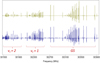 |
Fig. 1. Detail of the CH3SH rotational spectrum showing a-type R-branch transitions with J = 12 ← 11. The experimental spectrum is shown in the lower trace. A simulation of CH3SH transitions up to vt = 2 is shown in the upper trace. |
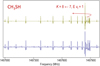 |
Fig. 2. Detail of the CH3SH rotational spectrum showing b-type Q-branch transitions with K = 8 ← 7 for the vt = 1 torsional state. The experimental spectrum is shown in the lower trace. A simulation of CH3SH transitions up to vt = 2 is shown in the upper trace. |
5. Discussion
We compared our current results with the parameters of the previous study (Xu et al. 2012) to have a more detailed picture of how the dataset extension affects the low order parameters in the RAM Hamiltonian model of CH3SH. In view of rather large differences in datasets and sets of high order torsion-rotational parameters, we limit the comparison of parameters up to fourth order only in Table 1. It should be noted that some parameter and operator expressions in Table 1 have changed in comparison with Table A.1. This is caused by the fact that the general Hamiltonian form (1), which is encoded in the RAM36 program, does not allow modification of the coefficient in front of the expression. Thus all coefficients historically adopted for a number of terms (such as minus sign in front of the quartic centrifugal distortion terms) are absorbed in the parameter values. For the purpose of the current comparison, we have recalculated all differing parameters to the form which conforms with results of Xu et al. (2012). As we can see from Table 1, there are no big changes either in the rotational constants or in the main internal rotational parameters V3, ρ, and F. In addition, many torsion–rotation distortion parameters of the fourth order agree well with previous results of Xu et al. (2012). The most noticeable differences are observed for ΔJK, Fbc, and D3bc, for which the signs changed. On one hand, this may be caused by the difference in the fourth order parameter sets. Indeed, in the current Hamiltonian model we do not use DabJ and DabK, which are present in the Xu et al. (2012) Hamiltonian model. On the other hand, this may be a consequence of additional correlation problems in the Xu et al. (2012) parameter set, where the number of fourth order parameters exceeds by 2 the maximum number of determinable parameters for this order as predicted by the reduction scheme proposed by Nakagawa et al. (1987). In any case, looking at the rather good agreement between many torsion–rotation distortion parameters of fourth order, it seems unlikely that the sign changes in ΔJK, Fbc, and D3bc are caused by the difference in the datasets.
One more issue, which should be discussed in connection with the current parameter set, is the expansion of the torsional potential function. It is seen from the comparison of the V3, V6, V9, V12 values that our expansion of the potential function is far from smooth convergence. In the previous study (Xu et al. 2012), the convergence of the potential function expansion raised only minor suspicion since V6 and V9 were of the same order (−0.572786(15) cm−1 and 0.205603(31) cm−1, respectively), whereas problems in the expansion convergence are more obvious in the present study because V9 is larger than V6, and V12 is larger than V9. It is known that the expansion coefficients of the torsional potential function may be highly correlated with Fermi-type couplings with small amplitude vibrations (Moazzen-Ahmadi 2002; Gascooke & Lawrance 2015). Thus, the current potential function behavior may be explained by the intervibrational interactions with the low lying small amplitude vibrational modes in methyl mercaptan. Indeed, the study of Lees et al. (2016) revealed strong torsion-vibrational resonant coupling between the vt = 4 torsional state and the CS stretching vibrational state of methyl mercaptan. The higher values of J and K accessed in the present study may give rise to a larger amount of perturbations between small amplitude vibrations and higher excited torsional states, and these perturbations can be transfered down to lower excited torsional states through intertorsional interactions. Our first attempts to include in the Hamiltonian model explicit interactions with low lying vibrational states lead to significant reductions in the V9 and V12 values, thus supporting the explanation above. This analysis of MW, FIR, and mid-IR spectra of the CS stretch state of methyl mercaptan is ongoing, and results will be presented elsewhere in due course.
6. Spectroscopic database
One outcome of the present work is a list of transitions calculated from the parameters of our final fit. This list includes information on transition quantum numbers, transition frequencies, calculated uncertainties, lower state energies, and transition strengths. Since extrapolation beyond the quantum number coverage of any given measured dataset rapidly becomes unreliable, especially in the case of molecules with large amplitude motions, we have chosen a torsional state limit of vt ≤ 2 and rotational limits of J ≤ 70 and |Ka| ≤ 20. As it was already mentioned, we label torsion–rotation levels by the free rotor quantum number m, the overall rotational angular momentum quantum number J, and a signed value of Ka. For convenience, a Kc value is also given but it is simply recalculated from J and Ka values (Kc = J − |Ka| for Ka ≥ 0 and Kc = J − |Ka|+1 for Ka < 0). The m = 0, −3, 3/1, −2, 4 values correspond to A/E transitions of the vt = 0, 1, 2 torsional states respectively. The predictions range up to 2 THz, and we limit our predictions to transitions with uncertainties less than 0.1 MHz. Lower state energies are given, referenced to the J = 0 A-type vt = 0 level. This level was calculated to be 107.49563 cm−1 above the bottom of the torsional potential well. The line strengths in the present line list were calculated using the values μa = 1.312 D and μb = −0.758 D (Tsunekawa et al. 1989), which were recalculated to the RAM axis system of the current study. In addition, we provide the rotation-torsion part of the partition function Qrt(T) of methyl mercaptan calculated from first principles (Table 3), that is, via direct summation over the rotational-torsion states. The maximum value of the J quantum number for the energy levels taken for calculating the partition function is 90 and nvt = 11 torsional states were taken into account. The predictions, as well as line list of the dataset treated in the present work, can be found at the CDS.
7. Conclusions
We have presented a new study of rotational spectra in the lowest three torsional states of methyl mercaptan main isotoplog  SH using a rotation–torsion RAM Hamiltonian. In the current study, the dataset available in the literature was augmented by new measurements in the 49−510 GHz range as well as new assignments in the 1.1−1.8 THz range. The set of 124 RAM Hamiltonian parameters fit with a weighted rms deviation of 0.72 the dataset of 6965 MW and 16 345 FIR line frequencies, which sample both A and E species of the vt = 0, 1, 2 torsional states with J ≤ 61 and Ka ≤ 18 and which cover the frequency range from 7 GHz to 1.8 THz for MW lines and up to 482 cm−1 for FIR lines. Based on these results, reliable frequency predictions were produced for astrophysical use up to 2 THz. These are available as supplementary material to this article. The predictions, as well as other supplementary files, will also be available in the Cologne Database for Molecular Spectroscopy1, CDMS (Endres et al. 2016).
Acknowledgments
The present study was supported by the Deutsche Forschungsgemeinschaft (DFG) in the framework of the collaborative research grant SFB 956 (project ID 184018867), sub-project B3. O.Z. is funded by the DFG via the Gerätezentrum “Cologne Center for Terahertz Spectroscopy” (project ID SCHL 341/15-1). The research in Kharkiv was carried out under support of the Volkswagen foundation. The assistance of the Science and Technology Center in the Ukraine is acknowledged (STCU partner project P686). L.H.X. and R.M.L. received support from the Natural Sciences and Engineering Research Council of Canada.
References
- Alekseev, E. A., Motiyenko, R. A., & Margules, L. 2012, Radio Phys. Radio Astron., 3, 75 [NASA ADS] [CrossRef] [Google Scholar]
- Anderson, D. E., Bergin, E. A., Maret, S., & Wakelam, V. 2013, ApJ, 779, 141 [NASA ADS] [CrossRef] [Google Scholar]
- Bettens, F. L., Sastry, K. V. L. N., Herbst, E., et al. 1999, ApJ, 510, 789 [NASA ADS] [CrossRef] [Google Scholar]
- Bossa, J.-B., Ordu, M. H., Müller, H. S. P., Lewen, F., & Schlemmer, S. 2014, A&A, 570, A12 [NASA ADS] [CrossRef] [EDP Sciences] [Google Scholar]
- Cernicharo, J., Marcelino, N., Roueff, E., et al. 2012, ApJ, 759, L43 [NASA ADS] [CrossRef] [Google Scholar]
- Charnley, S. B. 1997, ApJ, 481, 396 [NASA ADS] [CrossRef] [Google Scholar]
- Drozdovskaya, M. N., van Dishoeck, E. F., Jørgensen, J. K., et al. 2018, MNRAS, 476, 4949 [NASA ADS] [CrossRef] [Google Scholar]
- Endres, C. P., Schlemmer, S., Schilke, P., Stutzki, J., & Müller, H. S. P. 2016, J. Mol. Spectrosc., 327, 95 [Google Scholar]
- Gascooke, J. R., & Lawrance, W. D. 2015, J. Mol. Spectrosc., 318, 53 [CrossRef] [Google Scholar]
- Gibb, E., Nummelin, A., Irvine, W. M., Whittet, D. C. B., & Bergman, P. 2000, ApJ, 545, 309 [NASA ADS] [CrossRef] [PubMed] [Google Scholar]
- Hatchell, J., Thompson, M. A., Millar, T. J., & MacDonald, G. H. 1998a, A&AS, 133, 29 [NASA ADS] [CrossRef] [EDP Sciences] [Google Scholar]
- Hatchell, J., Thompson, M. A., Millar, T. J., & MacDonald, G. H. 1998b, A&A, 338, 713 [Google Scholar]
- Herbst, E., Messer, J. K., Lucia, F. C. D., & Helminger, P. 1984, J. Mol. Spectrosc., 108, 42 [Google Scholar]
- Hougen, J. T., Kleiner, I., & Godefroid, M. 1994, J. Mol. Spectrosc., 163, 559 [Google Scholar]
- Ilyushin, V. V., Kisiel, Z., Pszczókowski, L., Mäder, H., & Hougen, J. T. 2010, J. Mol. Spectrosc., 259, 26 [NASA ADS] [CrossRef] [Google Scholar]
- Ilyushin, V. V., Endres, C. P., Lewen, F., Schlemmer, S., & Drouin, B. J. 2013, J. Mol. Spectrosc., 290, 31 [Google Scholar]
- Kirtman, B. 1962, J. Chem. Phys., 37, 2516 [NASA ADS] [CrossRef] [Google Scholar]
- Kleiner, I. 2010, J. Mol. Spectrosc., 260, 1 [Google Scholar]
- Kojima, T. 1960, J. Phys. Soc. Jpn., 15, 1284 [NASA ADS] [CrossRef] [Google Scholar]
- Kojima, T., & Nishikawa, T. 1957, J. Phys. Soc. Jpn., 12, 680 [NASA ADS] [CrossRef] [Google Scholar]
- Kolesniková, L., Tercero, B., Cernicharo, J., et al. 2014, ApJ, 784, L7 [NASA ADS] [CrossRef] [Google Scholar]
- Lees, R. M., & Baker, J. G. 1968, J. Chem. Phys., 48, 5299 [NASA ADS] [CrossRef] [Google Scholar]
- Lees, R. M., & Mohammadi, M. A. 1980, Can. J. Phys., 58, 1640 [NASA ADS] [Google Scholar]
- Lees, R. M., Xu, L.-H., & Billinghurst, B. E. 2016, J. Mol. Spectrosc., 319, 30 [CrossRef] [Google Scholar]
- Lees, R. M., Xu, L.-H., & Billinghurst, B. E. 2018, J. Mol. Spectrosc., 352, 45 [CrossRef] [Google Scholar]
- Linke, R. A., Frerking, M. A., & Thaddeus, P. 1979, ApJ, 234, L139 [NASA ADS] [CrossRef] [Google Scholar]
- Majumdar, L., Gratier, P., Vidal, T., et al. 2016, MNRAS, 458, 1859 [NASA ADS] [CrossRef] [Google Scholar]
- Moazzen-Ahmadi, N. 2002, J. Mol. Spectrosc., 214, 144 [CrossRef] [Google Scholar]
- Müller, H. S. P., Belloche, A., Xu, L.-H., et al. 2016, A&A, 587, A92 [NASA ADS] [CrossRef] [EDP Sciences] [Google Scholar]
- Nakagawa, K., Tsunekawa, S., & Kojima, T. 1987, J. Mol. Spectrosc., 126, 329 [NASA ADS] [CrossRef] [Google Scholar]
- Ruffle, D. P., Hartquist, T. W., Caselli, P., & Williams, D. A. 1999, MNRAS, 306, 691 [NASA ADS] [CrossRef] [Google Scholar]
- Sastry, K. V. L. N., Herbst, E., Booker, R. A., & Lucia, F. C. D. 1986, J. Mol. Spectrosc., 116, 120 [NASA ADS] [CrossRef] [Google Scholar]
- Solimene, N., & Dailey, B. P. 1955, J. Chem. Phys., 23, 124 [NASA ADS] [CrossRef] [Google Scholar]
- Tsunekawa, S., Taniguchi, I., Tambo, A., et al. 1989, J. Mol. Spectrosc., 134, 63 [NASA ADS] [CrossRef] [Google Scholar]
- Turner, B. E. 1977, ApJ, 213, L75 [NASA ADS] [CrossRef] [Google Scholar]
- Vance, S., Christensen, L. E., Webster, C. R., & Sung, K. 2011, Planet. Space Sci., 59, 299 [NASA ADS] [CrossRef] [Google Scholar]
- Vastel, C., Quénard, D., Le Gal, R., et al. 2018, MNRAS, 478, 5514 [NASA ADS] [CrossRef] [Google Scholar]
- Wakelam, V., Hersant, F., & Herpin, F. 2011, A&A, 529, A112 [NASA ADS] [CrossRef] [EDP Sciences] [Google Scholar]
- Xu, L.-H., Fisher, J., Lees, R. M., et al. 2008, J. Mol. Spectrosc., 251, 305 [NASA ADS] [CrossRef] [Google Scholar]
- Xu, L.-H., Lees, R. M., Crabbe, G. T., et al. 2012, J. Chem. Phys., 137, 104313 [NASA ADS] [CrossRef] [Google Scholar]
- Zakharenko, O., Lewen, F., Ilyushin, V. V., et al. 2019, A&A, 621, A114 [NASA ADS] [CrossRef] [EDP Sciences] [Google Scholar]
Appendix A: Complementary table
Table A.1 summarizes the full set of 124 spectroscopic parameters determined in the present study.
Fit parameters of the RAM Hamiltonian for  SH molecule.
All Tables
All Figures
|
Fig. 1. Detail of the CH3SH rotational spectrum showing a-type R-branch transitions with J = 12 ← 11. The experimental spectrum is shown in the lower trace. A simulation of CH3SH transitions up to vt = 2 is shown in the upper trace. |
| In the text | |
|
Fig. 2. Detail of the CH3SH rotational spectrum showing b-type Q-branch transitions with K = 8 ← 7 for the vt = 1 torsional state. The experimental spectrum is shown in the lower trace. A simulation of CH3SH transitions up to vt = 2 is shown in the upper trace. |
| In the text | |
Current usage metrics show cumulative count of Article Views (full-text article views including HTML views, PDF and ePub downloads, according to the available data) and Abstracts Views on Vision4Press platform.
Data correspond to usage on the plateform after 2015. The current usage metrics is available 48-96 hours after online publication and is updated daily on week days.
Initial download of the metrics may take a while.