| Issue |
A&A
Volume 628, August 2019
|
|
|---|---|---|
| Article Number | A120 | |
| Number of page(s) | 8 | |
| Section | Atomic, molecular, and nuclear data | |
| DOI | https://doi.org/10.1051/0004-6361/201935593 | |
| Published online | 15 August 2019 | |
New study of the line profiles of sodium perturbed by H2⋆
1
GEPI, Observatoire de Paris, PSL Research University, UMR 8111, CNRS, Sorbonne Paris Cité, 61, Avenue de l’Observatoire, 75014 Paris, France
e-mail: This email address is being protected from spambots. You need JavaScript enabled to view it.
2
Institut d’Astrophysique de Paris, UMR7095, CNRS, Université Paris VI, 98bis Boulevard Arago, Paris, France
3
Laboratoire de Physique et de Chimie Quantique, Université de Toulouse (UPS) and CNRS, 118 route de Narbonne, 31400 Toulouse, France
4
Leiden Observatory, Leiden University, Postbus 9513, 2300 RA Leiden, The Netherlands
Received:
1
April
2019
Accepted:
2
July
2019
Abstract
The opacity of alkali atoms, most importantly of Na and K, plays a crucial role in the atmospheres of brown dwarfs and exoplanets. We present a comprehensive study of Na–H2 collisional profiles at temperatures from 500 to 3000 K, the temperatures prevailing in the atmosphere of brown dwarfs and Jupiter-mass planets. The relevant H2 perturber densities reach several 1019 cm−3 in hot (Teff ≳ 1500 K) Jupiter-mass planets and can exceed 1020 cm−3 for more massive or cooler objects. Accurate pressure-broadened profiles that are valid at high densities of H2 should be incorporated into spectral models. Unified profiles of sodium perturbed by molecular hydrogen were calculated in the semi-classical approach using up-to-date molecular data. New Na–H2 collisional profiles and their effects on the synthetic spectra of brown dwarfs and hot Jupiters computed with petitCODE are presented.
Key words: line: profiles / molecular data / brown dwarfs
Opacity tables are only available at the CDS via anonymous ftp to cdsarc.u-strasbg.fr (130.79.128.5) or via http://cdsarc.u-strasbg.fr/viz-bin/qcat?J/A+A/628/A120
© N. F. Allard et al. 2019
 Open Access article, published by EDP Sciences, under the terms of the Creative Commons Attribution License (http://creativecommons.org/licenses/by/4.0), which permits unrestricted use, distribution, and reproduction in any medium, provided the original work is properly cited.
1. Introduction
Alkali atoms are an important class of absorbers for modeling and understanding the spectra of self-luminous objects such as brown dwarfs and directly imaged planets. The wings of the sodium and potassium resonance lines in the optical are particularly important because they serve as a source of pseudo-continuum opacity, reaching into the near-infrared (NIR) wavelengths in the case of potassium. The relevance of these alkali species for the atmospheres of such self-luminous objects is studied and discussed in detail in Burrows et al. (2001). Moreover, it has been shown that the exact shape of the wings of the alkali lines, especially the red wings of the K doublet, affects the atmospheric structure, and that different treatments of the line wings can lead to differences in the temperature profiles at larger pressures (see, e.g., Baudino et al. 2017).
The class of transiting exoplanets (especially the so-called hot Jupiters) is also affected by the presence of the alkalis. Key observations with space- and ground-based telescopes have shed light on the conditions and composition of their atmospheres. Sodium was first detected in the atmosphere of HD209458b (Charbonneau et al. 2002), and is now routinely detected in many hot Jupiters from the ground and from space at high and low resolution. For examples, see Snellen et al. (2008), and the compilation of spectra in Sing et al. (2016) and Pino et al. (2018). Recently, the wing absorption of sodium was probed from the ground with the FORS2 observations by Nikolov et al. (2018).
For irradiated gas planets of intermediate temperature, the absorption of stellar light by the Na and K doublet line wings in the optical represents an important heating source (e.g., Mollière et al. 2015). Moreover, in the absence of strong cloud absorption, Na and K are the only significant absorbers of the flux of the host star in the optical. For higher planetary temperatures (T ≳ 2000 K), additional absorption by metal oxides, hydrides, atoms, and ions can become important (see, e.g., Arcangeli et al. 2018; Lothringer et al. 2018 and Lothringer & Barman 2019). Coupling of Na and K abundance to energy transfer causes the atmospheric temperature structures of hot Jupiters to be very sensitive to the shapes of the Na and K doublet lines. For special chemical conditions where the planetary cooling opacity is low, the heating by alkali atoms can even create inversions (Mollière et al. 2015). For self-luminous planets, the alkali opacities are important by virtue of their line wings as well. The red wings of the K doublet line in particular can control the flux escaping the planets in the Y band, which can also affect the planetary structure (Baudino et al. 2017).
In continuation with Allard et al. (2016) we present new unified line profiles of neutral Na perturbed by H2 using ab initio Na–H2 potentials and transition dipole moments. In Allard et al. (2003) we presented absorption profiles of sodium perturbed by molecular hydrogen. The line profiles were calculated in a unified line shape semi-classical theory (Allard et al. 1999) using Rossi & Pascale (1985) pseudo-potentials. Reliable calculations of pressure broadening in the far spectral wings require accurate potential-energy curves describing the interaction of the ground and excited states of Na with H2. In Allard et al. (2003) and Tinetti et al. (2007) we presented the first applications of semi-classical profiles of sodium and potassium perturbed by molecular hydrogen to the modeling of brown dwarfs and extra-solar planets. The 3s − 3p resonance line profiles were calculated using the Rossi & Pascale (1985) pseudo-potentials (hereafter labeled RP85). Ab initio calculations of the potentials (hereafter labeled FS11) of Na–H2 were computed by one of us (FS) and compared to pseudo-potentials of Rossi & Pascale (1985) in Allard et al. (2012a). We highlighted the regions of interest near the Na–H2 quasi-molecular satellites for comparison with previous results described in Allard et al. (2003). We also compared with laboratory absorption spectra. We extended this work to other excited states to allow a comprehensive determination of the spectrum (Allard et al. 2012b). Nevertheless, tables of Na–H2 absorption coefficients which are currently used for the construction of model atmospheres and synthetic spectra which have been generated from the line profiles reported in Allard et al. (2003) needed to be up to date.
We have now extended the calculations of the Na–H2 potential energy surfaces to the 5s state, and improved the accuracy for lower states. The new ab initio calculations of the potentials are carried out for the C2v (T-shape) symmetry group and the C∞v (linear) symmetry group. In this paper we restrict our study to the resonance 3s–3p line and will use the potentials of the more excited states described in Sect. 2 for a subsequent paper devoted to the line profiles of the sodium lines in the NIR. In addition, the transition dipole moments for the resonance line absorption, as a function of the geometry of the Na–H2 system are presented. The improvement over our previous work (Allard et al. 2012a) consists in a better determination of the long-range part of the Na–H2 potential curves. The inclusion of the spin-orbit coupling together with this improvement allow the determination of the individual line widths of the two components of the resonance 3s-3p doublet (Sect. 3). We illustrate the evolution of the absorption spectra of Na–H2 collisional profiles for the densities and temperatures prevailing in the atmospheres of cool brown dwarf stars and extrasolar planets. The new opacity tables of Na–H2 have been incorporated into atmosphere calculations of self-luminous planets and hot Jupiters. The atmospheric models presented in Sect. 4 have been calculated with petitCODE, a well-tested code that solves for the 1D structures of exoplanet atmospheres in radiative-convective and thermochemical equilibrium. Gas and optionally cloud opacities can be included, and scattering is treated in the structure and spectral calculations. petitCODE is described in Mollière et al. (2015, 2017).
2. Na–H2 potentials including spin-orbit coupling
The ab initio calculations of the potentials (hereafter labeled S17) were carried out for the C2v (T-shape) symmetry group and the C∞v (linear) symmetry group in a wide range of distances R between the Na atom and the center-of-mass of the H2 molecule. The potentials were calculated with the MOLPRO package (Werner et al. 2012) and are shown in Figs. 1–3. In the calculation of the complex, the bond length of H2 was kept fixed at the equilibrium value re = 1.401 a.u. and the approach is along the z coordinate axis. As in our previous calculations on KH2 (Allard et al. 2007a) and NaH2 (Allard et al. 2012a), we used a single active electron description of the sodium atom complemented with a core polarisation operator to include the core response. The effective core potential is the ECP10SDF effective core potential of the Stuttgart group (Nicklass et al. 1995). The core-polarization uses the formulation of Müller et al. (1984) with the parameters α = 0.997  and ρc = 0.62 for the core polarizability and the cut-off parameter of the CPP operator, respectively (corresponding to the smooth cut-off expression defined in MOLPRO). We used relatively extensive Gaussian-type basis sets (GTOs) to describe the three active electrons, namely 8s5p6d8f4g for Na and an spdf AV5Z basis set for each hydrogen atom. With this basis set, the one-electron scheme for sodium describes the transitions to the excited states of Na with an accuracy better than 25 cm−1 up to 5s, as illustrated in Table 1 and provides a fair account of correlation for the electrons of H2.
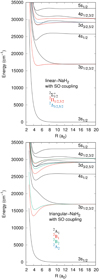 |
Fig. 1. Potential curves of the Na–H2 molecule for the C∞v (top) and C2v symmetries (bottom). For the C2v case, the symmetry labeling corresponds to the convention of the reference plane as that containing the molecule and may be different from that of previous publications. We note that states 12A2 and 42A1 correlated with the 3d asymptote are superimposed at the scale of the figure. |
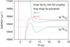 |
Fig. 2. Long-range potential curves of NaH2 correlated with the 3p1/2 and 3p3/2 asymptotes in C∞v symmetry. |
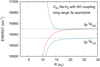 |
Fig. 3. Long-range potential curves of NaH2 correlated with the 3p1/2 and 3p3/2 asymptotes in C2v symmetry. |
Calculated atomic transitions and errors from the sodium ground state, as compared to multiplet-averaged experimental data (Moore 1971) (all in cm−1).
The determination of the electronic structure of NaH2 was carried out using the Multi Reference Configuration Interaction (MRCI) scheme of the MOLPRO package using the orbitals of  , which should provide an adequate Molecular Orbitals (MOs) description of the excited orbitals of the neutral molecule. For C∞v and C2v, the same symmetry subgroup is used in MOLPRO, namely C2v, the irreducible representations (irrep) of which correspond to Σ (and one Δ), Πx, Πy, and Δ states, respectively, for the linear case, and A1, B2, B1, and A2 states, respectively, for the isosceles case. The MRCI was generated from a Complete Active Space (CAS) involving three active electrons in 12, 8, 8, and 4 orbitals in each of the four irreps, respectively. This means that the generating CAS involves the valence orbitals of H2 as well as the 3s, 3p, 4s, 3d, 4p, 5s orbitals of sodium and even beyond. The MRCI space contains all simple and double excitations with respect to the CAS space (namely around 5 × 10⁵ configurations for each irrep).
Since we want to address spectral regions close to the line center of the atomic absorbing lines 3p and 4p, we incorporated SO coupling within a variant of the atom-in-molecule-like scheme introduced by Cohen & Schneider (1974). This scheme relies on a monoelectronic formulation of the spin-orbit coupling operator
 (1)
(1)
The total Hamiltonian Hel + HSO is expressed in the basis set of the eigenstates (here with  ) of the purely electrostatic Hamiltonian Hel. The spin-orbit coupling between the molecular many-electron doublet states Φkσ, approximated at this step as single determinants with the same closed shell
  H2 subpart, is isomorphic to that between the singly occupied molecular spin-orbitals ϕkσ, correlated with the six p spin-orbitals of the alkali atom (k labels the space part and σ = α, β labels the spin projection).
The Cohen and Schneider approximation consists in assigning these matrix elements to their asymptotic atomic values,
 (2)
(2)
The scheme makes no a priori assumption about the magnitude of spin-orbit coupling versus pure electrostatic interactions and allows general intermediate coupling. The main question for the applicability of the scheme in a basis of adiabatic states is the transferability of the atomic SO integrals to the molecular case, because of configurational mixing. Such a situation characterizes the short-distance interaction between the repulsive state correlated with the 3p configuration (either 22Σ+ or 22A1, depending on the symmetry) and the attractive 4s state (32Σ+ or 32A1). This means that the atomic spin-orbit coupling is not transferable at short distance in the adiabatic basis. Although this is not essential since the gap with the 2Π components becomes large at short distance, we have taken the variation of the coupling scheme of the 3p, 4s states into account in the following way. First, we achieved a diabatization of the 3p/4s anticrossing states in the 2Σ+ (resp 2A1) manifold, defining quasi-diabatic states  (k = 3p, 4s omitting the spin mention for convenience at this stage) as states with a constant transition dipole moment from the ground state. The adiabatic states are related to the latter through a 2 × 2 unitary transform at each distance R depending on a mixing angle θ. For the colinear case, the diabatic-to-adiabatic transformation is defined as
 (3)
(3)
 (4)
(4)
and the same transformation holds in the C2v symmetry for 2A1 states.
Assuming the conservation of the transition dipole moments from the ground state to the quasi-diabatic states along the internuclear distance, the transition moments to the adiabatic states can be related to the former ones. For instance, the transition moment from the ground state Φ0 to the MRCI spin-orbit-less eigenstate Φ3p is
 (5)
(5)
where μ(R) is the MRCI spin-orbit-less molecular adiabatic transition moment from the ground state to eigenstate Φ3p, and μat is its atomic or asymptotic value (2.537  ). Such a transformation was only carried for distances at which the molecular dipole moment is less than its atomic value. In the medium range around R = 10 − 11 a0, the adiabatic dipole transition moment reaches a very shallow maximum above its asymptotic value, that is 2.565
  for C∞v and 2.549
  for C2v. We note that complementarily, the Φ4s state, asymtotically characterized by a vanishing transition dipole moment, acquires a non-zero coupling with the ground state with a sinθ dependency. The evolution of the mixing along the internuclear distance is shown in Fig. 4. We obtain a 8 × 8 spin-orbit coupling matrix for the 3p/4s states, which is given in the Appendix.
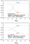 |
Fig. 4. Coefficients (cos θ and sin θ) of the 3p/4p diabatization in C∞v (top) and C2v symmetries (bottom). |
The spin-orbit energy splitting  of the 3p levels of sodium is 17.19 cm−1 (=
 ) (Moore 1971). No such diabatization was considered for the 4p configuration which has been treated via a 6 × 6 coupling matrix (e.g cosθ = 1) and a ζ constant equal to two third of the 5.58 cm−1 experimental splitting of the 4p manifold (Moore 1971). Spin-orbit coupling for the 3d configuration has been neglected. The diagonalization of the total Hel + HSO matrix at each internuclear distance provides the final energies
  and eigenstates
  .
.
The transition dipole moments shown in Fig. 5 between the spin-orbit states were determined by recombining the adiabatic MRCI dipole moments over the coefficients  of the spin-orbit states
  ,
,
 (6)
(6)
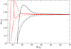 |
Fig. 5. Transition dipole moment for the B-X (full line), A2P3/2-X (dotted line), and A2P1/2-X (dashed line) transitions of the Na-H2 molecule for the C∞v (red curves) and C2v symmetries (black curves); B-X (full line), A2P3/2 − X (dotted line), and A2P1/2 − X (dashed line). |
In the following section, we only focus on the states correlated with the 3p manifold which determine the Na resonance lines. We evaluate the line parameters and collisional profiles for relevant temperatures and densities that are appropriate for modeling brown dwarf stars and hot-Jupiter-mass planets.
3. Temperature and density dependence of the Na resonance lines
In Allard et al. (1999), we derived a classical path expression for a pressure-broadened atomic spectral line shape that allows for an electric dipole moment that is dependent on the position of perturbers. This treatment has improved the comparison of synthetic spectra of brown dwarfs with observations (Allard et al. 2003, 2007b). This approach to calculating the spectral line profile requires knowledge of molecular potentials with high accuracy because the shape and strength of the line profile are very sensitive to the details of the molecular potential curves describing the Na–H2 collisions. Sodium is the most abundant alkali in cool dwarf atmospheres and is mostly responsible for the shape of the optical spectrum. With precise potentials and a complete line shape theory, major improvements in the theoretical description of pressure broadening have been made compared to the commonly used van der Waals broadening in the impact approximation (Burrows & Volobuyev 2003; Allard et al. 2003, 2012a,b).
3.1. Study of the line parameters
The impact theories of pressure broadening (Baranger 1958; Kolb & Griem 1958) are based on the assumption of sudden collisions (impacts) between the radiator and perturbing atoms, and are valid when frequency displacements Δ ω = ω − ω0 and gas densities are sufficiently small.
In impact broadening, the duration of the collision is assumed to be small compared to the interval between collisions, and the results describe the line within a few line widths of center. One outcome of our unified approach is that we may evaluate the difference between the impact limit and the general unified profile, and establish with certainty the region of validity of an assumed Lorentzian profile. In the planetary and brown dwarf upper atmospheres the H2 density is of the order of 1016 cm−3 in the region of line core formation.
The line parameters presented in Allard et al. (2007c, 2012a,b) were obtained using the pseudo-potentials of Rossi & Pascale (1985). To predict the impact parameters the intermediate- and long-range part of the potential energies need to be accurately determined. While the ab initio potentials presented in Allard et al. (2012a) allowed a better determination of the line wing, they were not accurate enough to determine the line parameters. With the improved potentials the half width at half-maximum w is linearly dependent on H2 density, and a power law in temperature is given for the D1 line by
 (7)
(7)
and for the D2 line is given by
 (8)
(8)
where w is in cm−1, nH2 in cm−3, and T in K. These expressions accurately represent the numerical results as shown in Fig. 6, and may be used to compute the widths for temperatures of stellar or planetary atmospheres from 500 up to at least 3000 K.
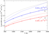 |
Fig. 6. Variation with temperature of the half-width of the D2 (blue curves) and D1 (red curves) lines of Na I perturbed by H2 collisions. New ab initio potentials (full line), pseudo-potentials of Rossi & Pascale (1985) (dashed lines), and the van der Waals potential (black dotted lines). |
3.2. Line satellite
Since the first Na–H2 pseudo-potentials were obtained by Rossi & Pascale (1985), significant progress in the description of NaH2 potentials has been achieved by Burrows & Volobuyev (2003), Santra & Kirby (2005) and Allard et al. (2012a). Blue satellite bands in alkali-He/H2 profiles can be predicted from the maxima in the difference potentials ΔV for the B-X transition. Figures 1 and 2 of Allard et al. (2012a) present the ab initio potential curves without spin-orbit coupling for the 3s and 3p of S11 compared to pseudo-potentials of RP85. It is seen there that the major difference with respect to S11 is that RP85 potentials are systematically less repulsive. This difference affects the blue satellite position. The NaH2 line satellite is closer to the main line than obtained with RP85 (Fig. 5 of Allard et al. 2012a). We observe this effect on synthetic spectra in the following section. On the red side, the NaH2 wings match the profiles from the RP85 potentials.
Figures 7–9 show the sensitivity of the line wings to pressure and temperature. The density effect on the shape of the blue wing is highly significant when the H2 density becomes larger than 1020 cm−3. We notice a first line satellite at 5170 Å in Fig. 7. A second satellite due to multiple-perturber effects appears as a shoulder at about 4800 Å for nH2 = 1021 cm−3. The density dependence of the far blue wing arises from multiple-perturber effects and is not linear in density. Figures 8 and 9 show the absorption cross section of the resonance line of Na compared to the Lorentzian profiles calculated using the line widths presented in Fig. 6, for T = 1000 K. The blue line wings shown in Fig. 8 are almost unchanged with increasing temperature whereas the red wings extend very far as temperature increases.
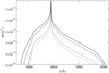 |
Fig. 7. Variation with the density of H2 of the D2 component (from top to bottom nH2 = 1021, 5 × 10²⁰, 1020 and 5 × 1019 cm−3). The temperature is 1500 K. |
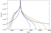 |
Fig. 8. Variation of the absorption cross sections of the 3s-3p D2 line component with temperature (from top to bottom T = 2500, 1500, 1000, and 600 K) for nH2 = 1021 cm−3. The Lorentzian profile for 1000 K is overplotted (black full line). |
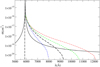 |
Fig. 9. Variation of the absorption cross sections of the 3s-3p D1 line component with temperature (from top to bottom T = 2500, 1500, 1000, and 600 K) for nH2 = 1021 cm−3. The Lorentzian profile for 1000 K is overplotted (black full line). |
3.3. Opacity tables
For the implementation of alkali lines perturbed by helium and molecular hydrogen in atmosphere codes, the line opacity is calculated by splitting the profile into a core component described with a Lorentzian profile, and the line wings computed using an expansion of the autocorrelation function in powers of density. Here we briefly review the use of a density expansion in the opacity tables.
The spectrum I(Δω) can be written as the Fourier transform (FT) of the dipole autocorrelation function Φ(s) (Allard et al. 1999),
 (9)
(9)
where Δω is the angular frequency difference from the unperturbed center of the spectral line. The autocorrelation function Φ(s) is calculated with the assumptions that the radiator is stationary in space, the perturbers are mutually independent, and in the adiabatic approach the interaction potentials give contributions that are scalar additive. This last simplifying assumption allows us to calculate the total profile I(Δω) when all the perturbers interact, as the FT of the Nth power of the autocorrelation function ϕ(s) of a unique atom-perturber pair. Therefore,
 (10)
(10)
that is to say, we neglect the interperturber correlations. We obtain for a perturber density np
 (11)
(11)
where decay of the autocorrelation function with time leads to atomic line broadening. When np is high, the spectrum is evaluated by computing the FT of Eq. (11). The real part of npg(s) damps Φ(s) for large s but this calculation is not feasible when extended wings have to be computed at low density because of the very slow decrease of the autocorrelation function. An alternative is to use the expansion of the spectrum I(Δω) in powers of the density described in Royer (1971).
We split the exponent g(s) in Eq. (11) into a “locally averaged part” gav(s) and an “oscillating part” gosc(s) by convolving g(s) with a Gaussian A(s):
 (12)
(12)
and
 (13)
(13)
where the asterisk stands for a convolution product.
We can write

At large values of s, g(s) becomes linear in s, gosc vanishes, and the oscillating part remains bounded which allows us to expand e−npgosc(s) in powers of npgosc(s); Eq. (11) becomes
![Mathematical equation: $$ \begin{aligned} \Phi (s) = e^{-n_{\rm p}g_{\mathrm{av}}(s)}[ 1 - n_{\rm p}g_{\mathrm{osc}}(s) + \frac{n_{\rm p}^2}{2!}[g_{\mathrm{osc}}(s)]^2 + \ldots ]. \end{aligned} $$](/articles/aa/full_html/2019/08/aa35593-19/aa35593-19-eq29.gif) (14)
(14)
The complete profile is given by the FT of Eq. (14):
![Mathematical equation: $$ \begin{aligned} I(\Delta \omega ) = I_c(\Delta \omega )*[\delta (\Delta \omega ) - n_{p}I_w(\Delta \omega ) + \frac{n_{p}^2}{2!}[I_w(\Delta \omega )]^{*2} + \ldots ] , \end{aligned} $$](/articles/aa/full_html/2019/08/aa35593-19/aa35593-19-eq30.gif) (15)
(15)
where Ic(Δω) = FT[e−npgav(s)] forms the core of the line profile and Iw(Δω) = FT[gosc(s)] is responsible for the wing.
This method gives the same results as the FT of the general autocorrelation function (Eq. (11) without density expansion) at higher densities and has the advantage of including multiperturber effects at very low density when the general calculation is not feasible (see, e.g., Allard & Alekseev 2014). The impact approximation determines the asymptotic behavior of the unified line shape correlation function. In this way the results described here are applicable to a more general line profile and opacity evaluation for the same perturbers at any given layer in the photosphere or planetary atmosphere.
When the expansion is stopped at the first order it is equivalent to the one-perturber approximation. Previous opacity tables were constructed to third order allowing us to obtain line profiles up to NH2 = 1019 cm−3. The new tables are constructed to a higher order allowing line profiles to NH2 = 1021 cm−3.
For a more direct comparison of the contributions of the two fine-structure components of the doublet it is convenient to use a cross-section σ associated to each component. The relationship between the computed cross-section and the normalized absorption coefficient given in Eq. (9) is
 (16)
(16)
where r0 is the classical radius of the electron, and f is the oscillator strength of the transition.
4. Astrophysical applications
4.1. Self-luminous atmosphere
In Fig. 10 we show the emission spectra for a cloud-free, self-luminous object (exoplanet or brown dwarf) at solar composition and varying effective temperature, calculated with petitCODE (Mollière et al. 2015, 2017). The atmospheric surface gravity was set to log(g) = 4.5, with g in units of cm s−2. The effective temperature was set to Teff = 800, 1500, and 2500 K, respectively. We calculated atmospheric structures and spectra using the old and new Na–H2 line profiles. The opacity of TiO, VO, and FeH was neglected to make the alkali lines visible also for the highest-temperature model. The difference in Na blue wing absorption is clearly visible. We also show the self-consistent temperature profiles of the atmospheres for these cases, as calculated with petitCODE. In the example shown here the effect of the change in opacity of the Na wings on the temperature profile is too small to be seen and the solid and dashed lines overlap.
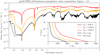 |
Fig. 10. Emission spectra for cloud-free, self-luminous objects (exoplanets or Brown Dwarfs) at solar composition and varying effective temperature, calculated with petitCODE (Mollière et al. 2015, 2017). The atmospheric surface gravity was set to log(g) = 4.5, with g in units of cm s−2. The black, orange, and red lines show the spectra for planets with Teff = 800, 1500, and 2500 K, respectively. Solid lines denote results obtained with the new Na wing profiles (presented in this paper), whereas dashed lines denote the results obtained with the Na lines reported in Allard et al. (2003). The inset plot shows the self-consistent temperature profiles for these cases, as calculated with petitCODE. In the example shown here the effect of the change in opacity of the Na wings is too small to be seen. |
4.2. Hot Jupiter
In Fig. 11 we show the transmission spectra for cloud-free hot-Jupiter exoplanets at solar composition for a planetary effective temperature of 1800 K, also calculated with petitCODE (Mollière et al. 2015, 2017). The planet mass and radius were chosen to be identical to the values of Jupiter, and an internal temperature of Tint = 200 K was used. The TiO/VO opacities were neglected. The host star was chosen to be a solar twin. We calculated atmospheric structures and spectra using the old and new NaH2 line profiles. The difference in Na blue wing absorption is clearly visible. We also show the self-consistent temperature profiles of the atmospheres for these cases, as calculated with petitCODE. In the example shown here the weaker absorption in the new line profiles leads to more green house heating in the deep layers of the atmosphere, while the upper layers are slightly cooler than what was obtained with the old line profiles.
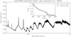 |
Fig. 11. Transmission radii for cloud-free, hot-Jupiter exoplanets at solar composition for a planetary effective temperature of 1800 K, calculated with petitCODE (Mollière et al. 2015, 2017). The planet mass and radius were chosen to be identical to the values of Jupiter, and an internal temperature of Tint = 200 K was used. The opacity of TiO and VO was neglected. The host star was chosen to be a solar twin. Solid lines denote results obtained with the new Na wing profiles (presented in this paper), whereas dashed lines denote the results obtained with the Na lines reported in Allard et al. (2003). The inset plot shows the self-consistent temperature profiles for these cases, as calculated with petitCODE. In the example shown here the weaker absorption in the new Na wing profiles leads to more greenhouse heating in the deep layers of the atmosphere, while the upper layers are slightly cooler than what was obtained with the old profiles. |
5. Conclusion
We performed theoretical calculations of the collisional profiles of the resonance lines of Na perturbed by H2 using a unified theory of spectral line broadening and high-quality ab initio potentials and transition moments. Figures 10 and 11 show that the perturbation of Na by H2 can be very important for the interpretation of visible spectra of brown dwarf and exoplanet atmospheres. We therefore suggest that the use of Lorentzian profiles is not appropriate for modeling the line wings, as Figs. 8 and 9 clearly show. Complete unified line profiles based on accurate atomic and molecular physics should be incorporated into analyses of exoplanet spectra when precise absorption coefficients are needed. Calculations are presented for the D1 and D2 lines from Teff = 500 K–3000 K with a step size of 500 K. Tables of the density expansion coefficients, an explanation of their use, and a program to produce line profiles to NH2 = 1021 cm−3 will be archived at the CDS.
References
- Allard, N. F., & Alekseev, V. A. 2014, Adv. Space Res., 54, 1248 [NASA ADS] [CrossRef] [Google Scholar]
- Allard, N. F., Royer, A., Kielkopf, J. F., & Feautrier, N. 1999, Phys. Rev. A, 60, 1021 [NASA ADS] [CrossRef] [Google Scholar]
- Allard, N. F., Allard, F., Hauschildt, P. H., Kielkopf, J. F., & Machin, L. 2003, A&A, 411, L473 [NASA ADS] [CrossRef] [EDP Sciences] [Google Scholar]
- Allard, N. F., Spiegelman, F., & Kielkopf, J. F. 2007a, A&A, 465, 1085 [NASA ADS] [CrossRef] [EDP Sciences] [Google Scholar]
- Allard, F., Allard, N. F., Homeier, D., et al. 2007b, A&A, 474, L21 [NASA ADS] [CrossRef] [EDP Sciences] [Google Scholar]
- Allard, N. F., Kielkopf, J. F., & Allard, F. 2007c, EPJ D, 44, 507 [Google Scholar]
- Allard, N. F., Spiegelman, F., Kielkopf, J. F., Tinetti, G., & Beaulieu, J. P. 2012a, A&A, 543, A159 [NASA ADS] [CrossRef] [EDP Sciences] [Google Scholar]
- Allard, N. F., Kielkopf, J. F., Spiegelman, F., Tinetti, G., & Beaulieu, J. P. 2012b, EAS Publ. Ser., 58, 239 [Google Scholar]
- Allard, N. F., Spiegelman, F., & Kielkopf, J. F. 2016, A&A, 589, A21 [NASA ADS] [CrossRef] [EDP Sciences] [Google Scholar]
- Arcangeli, J., Désert, J.-M., Line, M. R., et al. 2018, ApJ, 855, L30 [NASA ADS] [CrossRef] [Google Scholar]
- Baranger, M. 1958, Phys. Rev., 111, 481 [NASA ADS] [CrossRef] [MathSciNet] [Google Scholar]
- Baudino, J.-L., Mollière, P., Venot, O., et al. 2017, ApJ, 850, 150 [NASA ADS] [CrossRef] [Google Scholar]
- Burrows, A., & Volobuyev, M. 2003, ApJ, 583, 985 [NASA ADS] [CrossRef] [Google Scholar]
- Burrows, A., Hubbard, W. B., Lunine, J. I., & Liebert, J. 2001, Rev. Mod. Phys., 73, 719 [Google Scholar]
- Charbonneau, D., Brown, T. M., Noyes, R. W., & Gilliland, R. L. 2002, ApJ, 568, 377 [NASA ADS] [CrossRef] [Google Scholar]
- Cohen, J. S., & Schneider, B. 1974, J. Chem. Phys., 61, 3230 [NASA ADS] [CrossRef] [Google Scholar]
- Kolb, A. C., & Griem, H. 1958, Physical Review, 111, 514 [NASA ADS] [CrossRef] [Google Scholar]
- Lothringer, J. D., & Barman, T. S. 2019, ApJ, 876, 69 [NASA ADS] [CrossRef] [Google Scholar]
- Lothringer, J. D., Barman, T., & Koskinen, T. 2018, ApJ, 866, 27 [NASA ADS] [CrossRef] [Google Scholar]
- Mollière, P., van Boekel, R., Dullemond, C., Henning, T., & Mordasini, C. 2015, ApJ, 813, 47 [NASA ADS] [CrossRef] [Google Scholar]
- Mollière, P., van Boekel, R., Bouwman, J., et al. 2017, A&A, 600, A10 [NASA ADS] [CrossRef] [EDP Sciences] [Google Scholar]
- Moore, C. E. 1971, Bull. Am. Astron. Soc., 3, 154 [NASA ADS] [Google Scholar]
- Müller, W., Flesch, J., & Meyer, W. 1984, J. Chem. Phys., 80, 3297 [NASA ADS] [CrossRef] [Google Scholar]
- Nicklass, A., Dolg, M., Stoll, H., & Preuss, H. 1995, J. Chem. Phys., 102, 8942 [Google Scholar]
- Nikolov, N., Sing, D. K., Fortney, J. J., et al. 2018, Nature, 557, 526 [NASA ADS] [CrossRef] [Google Scholar]
- Pino, L., Ehrenreich, D., Wyttenbach, A., et al. 2018, A&A, 612, A53 [NASA ADS] [CrossRef] [EDP Sciences] [Google Scholar]
- Rossi, F., & Pascale, J. 1985, Phys. Rev. A, 32, 2657 [NASA ADS] [CrossRef] [PubMed] [Google Scholar]
- Royer, A. 1971, Phys. Rev. A, 3, 2044 [Google Scholar]
- Santra, R., & Kirby, K. 2005, J. Chem. Phys., 123, 214309 [NASA ADS] [CrossRef] [PubMed] [Google Scholar]
- Sing, D. K., Fortney, J. J., Nikolov, N., et al. 2016, Nature, 529, 59 [NASA ADS] [CrossRef] [Google Scholar]
- Snellen, I. A., Albretch, S., Mooij, E. J. W., & Poole, R. S. L. 2008, A& A, 487, 357 [Google Scholar]
- Tinetti, G., Vidal-Madjar, A., Liang, M.-C., et al. 2007, Nature, 448, 169 [NASA ADS] [CrossRef] [PubMed] [Google Scholar]
- Werner, H.-J., Knowles, P. J., Knizia, G., Manby, F. R., & Schütz, M. 2012, WIREs Comput. Mol. Sci., 2, 242 [CrossRef] [Google Scholar]
Appendix A: SO matrix for 3p and 4s states
All Tables
Calculated atomic transitions and errors from the sodium ground state, as compared to multiplet-averaged experimental data (Moore 1971) (all in cm−1).
All Figures
|
Fig. 1. Potential curves of the Na–H2 molecule for the C∞v (top) and C2v symmetries (bottom). For the C2v case, the symmetry labeling corresponds to the convention of the reference plane as that containing the molecule and may be different from that of previous publications. We note that states 12A2 and 42A1 correlated with the 3d asymptote are superimposed at the scale of the figure. |
| In the text | |
|
Fig. 2. Long-range potential curves of NaH2 correlated with the 3p1/2 and 3p3/2 asymptotes in C∞v symmetry. |
| In the text | |
|
Fig. 3. Long-range potential curves of NaH2 correlated with the 3p1/2 and 3p3/2 asymptotes in C2v symmetry. |
| In the text | |
|
Fig. 4. Coefficients (cos θ and sin θ) of the 3p/4p diabatization in C∞v (top) and C2v symmetries (bottom). |
| In the text | |
|
Fig. 5. Transition dipole moment for the B-X (full line), A2P3/2-X (dotted line), and A2P1/2-X (dashed line) transitions of the Na-H2 molecule for the C∞v (red curves) and C2v symmetries (black curves); B-X (full line), A2P3/2 − X (dotted line), and A2P1/2 − X (dashed line). |
| In the text | |
|
Fig. 6. Variation with temperature of the half-width of the D2 (blue curves) and D1 (red curves) lines of Na I perturbed by H2 collisions. New ab initio potentials (full line), pseudo-potentials of Rossi & Pascale (1985) (dashed lines), and the van der Waals potential (black dotted lines). |
| In the text | |
|
Fig. 7. Variation with the density of H2 of the D2 component (from top to bottom nH2 = 1021, 5 × 10²⁰, 1020 and 5 × 1019 cm−3). The temperature is 1500 K. |
| In the text | |
|
Fig. 8. Variation of the absorption cross sections of the 3s-3p D2 line component with temperature (from top to bottom T = 2500, 1500, 1000, and 600 K) for nH2 = 1021 cm−3. The Lorentzian profile for 1000 K is overplotted (black full line). |
| In the text | |
|
Fig. 9. Variation of the absorption cross sections of the 3s-3p D1 line component with temperature (from top to bottom T = 2500, 1500, 1000, and 600 K) for nH2 = 1021 cm−3. The Lorentzian profile for 1000 K is overplotted (black full line). |
| In the text | |
|
Fig. 10. Emission spectra for cloud-free, self-luminous objects (exoplanets or Brown Dwarfs) at solar composition and varying effective temperature, calculated with petitCODE (Mollière et al. 2015, 2017). The atmospheric surface gravity was set to log(g) = 4.5, with g in units of cm s−2. The black, orange, and red lines show the spectra for planets with Teff = 800, 1500, and 2500 K, respectively. Solid lines denote results obtained with the new Na wing profiles (presented in this paper), whereas dashed lines denote the results obtained with the Na lines reported in Allard et al. (2003). The inset plot shows the self-consistent temperature profiles for these cases, as calculated with petitCODE. In the example shown here the effect of the change in opacity of the Na wings is too small to be seen. |
| In the text | |
|
Fig. 11. Transmission radii for cloud-free, hot-Jupiter exoplanets at solar composition for a planetary effective temperature of 1800 K, calculated with petitCODE (Mollière et al. 2015, 2017). The planet mass and radius were chosen to be identical to the values of Jupiter, and an internal temperature of Tint = 200 K was used. The opacity of TiO and VO was neglected. The host star was chosen to be a solar twin. Solid lines denote results obtained with the new Na wing profiles (presented in this paper), whereas dashed lines denote the results obtained with the Na lines reported in Allard et al. (2003). The inset plot shows the self-consistent temperature profiles for these cases, as calculated with petitCODE. In the example shown here the weaker absorption in the new Na wing profiles leads to more greenhouse heating in the deep layers of the atmosphere, while the upper layers are slightly cooler than what was obtained with the old profiles. |
| In the text | |
Current usage metrics show cumulative count of Article Views (full-text article views including HTML views, PDF and ePub downloads, according to the available data) and Abstracts Views on Vision4Press platform.
Data correspond to usage on the plateform after 2015. The current usage metrics is available 48-96 hours after online publication and is updated daily on week days.
Initial download of the metrics may take a while.