| Issue |
A&A
Volume 628, August 2019
|
|
|---|---|---|
| Article Number | A63 | |
| Number of page(s) | 5 | |
| Section | Atomic, molecular, and nuclear data | |
| DOI | https://doi.org/10.1051/0004-6361/201935153 | |
| Published online | 08 August 2019 | |
An experimental test for effective medium approximations (EMAs)
Porosity determination for ices of astrophysical interest
Centro de Tecnologías Físicas, Universitat Politècnica de València, Plaza Ferrándiz-Carbonell, 03801 Alcoy, Spain
e-mail: This email address is being protected from spambots. You need JavaScript enabled to view it.
Received:
29
January
2019
Accepted:
2
July
2019
Abstract
Aims. The effective medium approximations (EMAs), or the Lorentz–Lorenz, Maxwell-Garnett, and Bruggeman models, largely used to obtain optical properties and porosities of pure and ice mixtures, have been experimentally tested in this work. The efficiency of these approximations has been studied by obtaining the porosity value for carbon dioxide ice grown at low temperatures. An explanation of the behaviour of the experimental results for all temperatures is given. The analysis carried out for CO2 can be applied to other molecules.
Methods. An optical laser interference technique was carried out using two laser beams falling on a growing film of ice at different incident angles which allowed us to determine the refractive index and the thickness of the film. The mass deposited is recorded by means of a quartz crystal microbalance. Porosity is determined from its equational definition by using the experimental density previously obtained.
Results. From the experimental results of the refractive index and density, porosity values for carbon dioxide ice films grown on a cold surface at different temperatures of deposition have been calculated and compared with the results obtained from the EMA equations, and with recent experimental results.
Conclusion. The values of porosity obtained with the EMA models and experimentally, show similar trends. However, theoretical values overestimate the experimental results. We can conclude that using the EMAs to obtain this parameter from an ice mixture must be carefully considered and, if possible, an alternative experimental procedure that allows comparisons to be made should be used.
Key words: astrochemistry / methods: laboratory: solid state / ISM: molecules
© ESO 2019
1. Introduction
There are two main reasons why porosity is relevant to astrochemistry. Firstly, porous ices trap molecules inside the structure causing an offset in the temperature at which the molecules trapped are released (not the sublimation temperature, which remains unaltered). Therefore, the temperature at which these molecules become potential reactives, for instance, in protostellar clouds (Rodgers & Charnley 2003; Viti et al. 2004; Herbst 2005; Garrod et al. 2008; Aikawa et al. 2008) is also altered. Secondly, its large surface area (absorption areas can be hundreds of m2 g−1) gives the ice the ability to trap significant amounts of volatiles and to act as catalysts for the formation of larger molecules greater than those that would form in the gas phase (Bartels-Rausch et al. 2012).
Bearing in mind that water is the most abundant molecule in the solid phase observed in the interstellar medium, the porosity it exhibits when formed at low temperatures has been the subject of intense studies (Rowland et al. 1991; Rowland & Devlin 1991; Keane et al. 2001; Palumbo 2006; Raut et al. 2007; Palumbo et al. 2010; Isokoski et al. 2014; Cazaux et al. 2015). Even though these studies exclusively deal with the porosity of water, other molecules of astrophysical interest also exhibit a porous structure; for example, CO2 ice (Luna et al. 2008) shows porosity and the ability to trap volatiles in spite of being processed thermally. In the case of CO2, the molecule of focus in this study, Edridge et al. (2013, and references therein) give an idea of the important role that this molecule plays in the chemistry within the interstellar medium.
Due to the interest in the porosity of ice and the difficulties of obtaining it experimentally, a theoretical model that reduces the number of parameters to be determined is of great interest. The effective medium approximations (EMAs) provide a set of equations for obtaining the physical parameters of a mixture of different materials from the corresponding values of the pure components. The parameters studied in the literature are roughness (Aspnes et al. 1979), electric conductivity in composite media (Stroud 1998), dielectric constants of heterogeneous materials (Niklasson et al. 1981; Luo 1997), and porosity of ices created in astrophysical conditions (Bossa et al. 2014).
The most widely used EMAs are the Maxwell Garnett (1904, 1906), Bruggeman (1935), and Lorentz–Lorenz (Lorentz 1880; Lorenz 1880), the last of which can be found in a more modern version in Born & Wolf (1999). An exhaustive study of the three models can be found in Markel’s works (Markel 2016a,b). These three EMAs were designed for binary mixtures, but were obtained from different theoretical frameworks. Niklasson et al. (1981) derived the Maxwell-Garnett and Bruggeman EMAs from new and unified theoretical frameworks, still for two components but introducing a study on the limits regarding the size of the inclusions to which both models could be applied. This framework was improved by Luo (1997) including mixtures of several components.
The porosity is defined by Eq. (1):
 (1)
(1)
where ρa represents the density of the material including the voids inside (porous) and ρi is for the bulk material.
In Westley et al. (1998) the porosity of vapour-deposited films of water ice were obtained in two ways: on the one hand by measuring density, which is obtained from the thickness of the sample and knowing the mass deposited from the change in frequency from a quartz crystal microbalance (QCMB), and using Eq. (1), and on the other hand by using the Lorentz–Lorenz equation (see Eq. (4) below) from the knowledge of the refractive index, finding that both results match within the error bars. In Bossa et al. (2014) the porosity of water is calculated from the experimental results of the refractive index by interferometry and introducing it in the Lorentz–Lorenz equation (see below). These results were compared with the porosity that can be inferred from the Maxwell-Garnett and Bruggeman EMAs. However, they emphasize the need to directly measure the density using a QCMB for proper evaluation of these theoretical models.
For the reason specified in the previous paragraph, this paper aims to check the use of the most well-known EMAs to measure the porosity of CO2 ice grown at different temperatures under astrophysical conditions. The technique used is based on the measurement of the deposited mass by means of a QCMB as suggested in Bossa et al. (2014). The experimental results obtained from the definition of porosity (Eq. (1)) will be compared with the theoretical results. Section 2 is a brief explanation of the models and equations of the most widely used EMAs. Section 3 details experiments and data analysis. Section 4 presents the results obtained, and the discussion is given in Sect. 5.
2. Effective medium approximations
The effective medium approximations are theories that allow us to compute the physical properties of a heterogeneous sample from its constituents. In this work, concerning porosity, one of the constituent must be vacuum. Depending on how the sample is structured, there are three models that will be explained in detail below.
2.1. Maxwell-Garnett
In the Maxwell-Garnett EMA the system can be represented as inclusions of an element A evenly distributed in a host medium B, forming a separated-grain structure. This structure can be observed in Fig. 1, which was obtained from Niklasson et al. (1981).
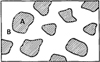 |
Fig. 1. Separated-grain microstructure for heterogeneous two-phase media. |
Following Bossa et al. (2014), the material can be treated as an effective medium, characterized by an effective dielectric constant (ϵeff) related to the refractive index by  . Hereafter we prefer to use na instead of neff; the latter is the usual form found in the literature on the subject, but the former can be found in astrophysical literature. Equation (2) would accomplish this purpose in the case of a porous material in which A is the vacuum with refractive index 1:
 (2)
(2)
Here, the parameter ni is the refractive index of the bulk matter, without voids, and the parameter p indicates the porosity. Knowing the refractive indices, the porosity can be calculated.
2.2. Bruggeman
The Bruggeman equation mathematically represents a symmetric conception of the matter in which all the components play the same role (there is neither host nor inclusion). This structure can be observed in Fig. 2, which was obtained from Niklasson et al. (1981).
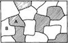 |
Fig. 2. Aggregate microstructure for a heterogenous two-phase media. |
Similar to the previous model, the porosity can be obtained from the equation (Bossa et al. 2014):
 (3)
(3)
All the parameters have the same meaning, as shown in Eq. (2). These two models were conceived in such a way that the size and separation distance are assumed to be smaller than the optical wavelength so that the medium behaves homogeneously.
2.3. Lorentz–Lorenz
This equation is another development, based on the works of Lorentz (1880) and Lorenz (1880) regarding the molecular theory of polarization. In this model matter is considered a collection of point-like polarizable atoms or molecules in a vacuum. The aim is to obtain the dielectric permittivity (i.e. the refractive index of the medium) produced by the above-mentioned entities.
The starting point of this model is different. While the first two models assume the validity of the Maxwell equations inside the composite, this model does not need this assumption and the permittivity is obtained from the concepts of polarizability of the individual molecules and polarization density. The following equation captures these concepts and relates all the parameters:
 (4)
(4)
Equation (4) is usually used to experimentally obtain the porosity of ices deposited at astrophysically relevant temperatures (Bossa et al. 2014). However, as in Eqs. (2) and (3), the only experimental parameter is the refractive index of the ice. A deeper study of the theoretical fundaments and a comparison of all three models can be found in Markel (2016a,b).
3. Experimental methods
Experiments were performed in a set-up described in detail in previous works (e.g. Satorre et al. 2018). It consists of a high vacuum (HV) chamber at 10−7 mbar base pressure, inside which a closed-cycle He cryostat cools down the sample holder close to 10 K. The temperature can be controlled up to room temperature with 0.5 K accuracy. Molecules are background-deposited onto a gold-plated QCMB. During deposition the pressure is maintained constant in the chamber, and a constant deposition rate is obtained. These parameters are related by the Sauerbrey (1959) equation (Δf = −S ⋅ Δm). In this equation Δf is the change in frequency, Δm represents the mass accreted onto the QCMB, and S is a specific constant for every QCMB. Two He–Ne laser beams (633 nm) impinge at the centre of the QCMB at two angles of incidence (α and β), forming two interference patterns during film growth. As the thickness and the refractive index are the same for both interference patterns, and the incidence angles are known, the refractive index can be calculated as
 (5)
(5)
where γ = Tα/Tβ is the quotient between the periods of the two interferential patterns obtained from each laser. Knowing the refractive index, the thickness is determined by
 (6)
(6)
where n is the refractive index of the medium, λ and β are respectively the wavelength and the incident angle, and qβ is the number of adjacent peaks. This equation, in the case of the interferential pattern, is obtained from the laser with an angle of incidence β. Samples are typically a few microns (μm) thick. The density was calculated by dividing the mass deposited per unit area (g cm−2), measured with the QCMB, by the thickness (cm), determined with the lasers. Praxair CO2 gas of purity 99.99% was used in all the experiments.
4. Results
The porosity of solid CO2 was calculated experimentally (with known density), and it was also theoretically derived (from the refractive index) using the EMA theories at temperatures ranging from 10 to 86 K. The experimental values, both n and ρ, correspond to those published in Satorre et al. (2008) updated with results obtained between 2009 and 2018 (Satorre et al. 2018).
Graphs in this section plot density, refractive index, and porosity vs. temperature of deposition. The error bars were obtained by taking the t-Student value with a significance level of 0.05. The solid lines in all graphs are indicative of the linear behaviour; it is not a linear fit.
4.1. Density
From Fig. 3 it is apparent that ρ (g cm−3) increases following the increase in CO2 ice deposition temperature. The result is an ice whose structure shows a porosity that varies with temperature, tending towards greater compaction at higher temperatures up to a stable value reached around 50 K.
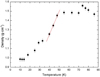 |
Fig. 3. Density of CO2 ice vs. deposition temperature. |
Schulze & Abe (1980) reported an increase in density at temperatures close to 10 K. In our work, density remains constant within the error bars from 10 K to 15 K. A slight tendency of decrease can be seen in this temperature range, but as it is within the error bars it does not indicate anything conclusive.
At 40 K there is an inflection point that separates two zones: below 40 K, the shape is similar to a staircase; above this temperature, a linear behaviour up to 50 K is observed. At 50 K the value of the density reaches a plateau and becomes constant (1.48 g cm−3), and then increases to a temperature of 74 K. At 74 K a gap is produced reaching the density a value of 1.56 g cm−3. From this temperature, the value of the density decreases until the plateau mentioned above is reached. The highest value obtained does not implicate the absence of porosity because the density is still lower than the highest value reported by Maass & Barnes (1926), 1.674 g cm−3 for crystalline structure at 90 K, which could indicate that a porous structure persists at these temperatures.
4.2. Refractive index
In Fig. 4 the behaviour shown is similar to that of the density for temperatures below 50 K. From this temperature the refractive index is not constant probably because the film presents structural changes. Similar quantitative values and qualitative behaviour can be found in Isokoski et al. (2014), where the refractive index also reduces its value at temperatures above 55 K and up to 70 K. Nevertheless, the reduction is within the uncertainty interval. At 75 K, the refractive index recovers the value obtained at 50 K.
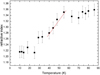 |
Fig. 4. Refractive index of CO2 ice vs. deposition temperature. |
4.3. Porosity
The porosity was obtained from the equational definition expressed mathematically by Eq. (1) and plotted in Fig. 5. For the ice density without voids, known as intrinsic density, the value of 1.67 g cm−3 is assigned in this work. This value was obtained by Maass & Barnes (1926) for a perfectly crystalline ice.
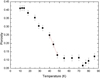 |
Fig. 5. Porosity of CO2 ice vs. deposition temperature. |
As observed in Fig. 5, the porosity shows the expected behaviour in accordance with the density. The curve displays three different behaviours: below 40 K the porosity displays the same staircase structure; between 40 K and 50 K it shows a linear behaviour with deposition temperature (red line in Fig. 5). In these two temperature ranges the decrease in the value of porosity is more pronounced in the 40 to 50 K zone than in zone below 40 K. Finally, above 55 K the porosity presents a constant value, with the exception of the three temperatures where the density displays a gap: 74, 77, and 80 K. In all cases the porosity is different to zero. At 86 K the porosity recovers the value reached at 55 K.
5. Discussion
In this section we will compare the results obtained from the EMAs with the experimental ones, and we will give an explanation to the behaviour shown by the density, the refraction index and the porosity when considering the increase of temperature at which the deposit is carried out.
5.1. Comparison of EMAs and experiments
Here we compare and discuss our experimental results and those obtained by the EMAs. To use Eqs. (2)–(4), ni is taken as 1.41 (Warren 1986), and the values of na are those in Sect. 4. Experimental (Sect. 4.3) and theoretical values are plotted in Fig. 6. The experimental and theoretical values obtained from Loeffler et al. (2016) for the case of background deposition have been included.
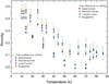 |
Fig. 6. Experimental and theoretical (EMAs) CO2 porosities obtained from Satorre et al. (2018) and Loeffler et al. (2016) at different deposition temperatures. At 30 K the Loeffler results obtained without thermal shield are also shown (empty dots). |
From a qualitative point of view the most remarkable observation concerning our results is that all three models show a similar behaviour to the experiment results up to 50 K. From 50 K onwards, the experimental values remain constant up to 70 K, whereas the theoretical values increase due to the reduction in the value of refractive index at the same temperature interval. From 70 to 86 K the gap obtained by the experimental density values, not reported in the refractive index values, causes greater disagreement between the two value sets.
From a quantitative point of view, it is worth noting the shift to higher values of porosity for all EMAs at all temperatures with respect to the experimental values, being in order of the displacement size from major to minor: Maxwell-Garnett, Bruggeman, and Lorentz–Lorenz.
It is also important to note that at 25 K the values obtained from the refractive index differ significantly from the other temperatures, being higher by almost 10% than the experimental value. Even at this temperature, the error bars associated with the experimental and theoretical values do not overlap. The only possible explanation we found was that at this temperature Escribano et al. (2013) detect signs of the presence of crystalline phase in the ice.
In Loeffler et al. (2016) new results for the refractive index and density of CO2 ice have been obtained experimentally via different deposition methods. For comparison purposes, we chose background deposition data, with and without thermal shield, to compute the experimental and theoretical (EMA) porosities. All the porosities obtained are lower than the values derived from Satorre et al. (2018) by up to 10%. For the highest temperatures, no porosity is obtained because Loeffler et al. (2016) present a density value slightly higher than the maximum value found for the intrinsic density by Maass & Barnes (1926), which is the value we used to calculate the porosity. Also in Loeffler et al. (2016), for 30 and 70 K, some experiments without thermal shield are carried out. Porosity calculated at 30 K is higher than that with thermal shield, but they do not reach the values derived from Satorre et al. (2018). At 70 K they are indistinguishable with or without thermal shield, and for this reason they are not present in Fig. 6. It can be observed, as in the results derived from Satorre et al. (2018), that the Loeffler et al. (2016) experimental values are lower than the theoretical values. Both sets of values decrease linearly from 15 to 60 K and appear to remain at a constant value up to 70 K. Another aspect to emphasize is that while the experimental measurements indicate a lack of porosity from 60 K, and possibly between 50 and 60 K, the theoretical measurements seem to indicate the presence of a minimum value for porosity, which is in agreement with the experimental results obtained via other methods (Schulze & Abe 1980). We think that the key issue is the value taken for the intrinsic density of the ice.
5.2. Explanation of CO2 ice density, refractive index, and porosity behaviour
The staircase form in Figs. 3–5 at T < 40 K is remarkable, and deserves special attention. In Schulze & Abe (1980) this behaviour was not observed for density; but it was in the isosteric adsorption energy of H2 on solid CO2 at low temperatures. As the deposition temperature increases, this step behaviour disappears progressively as the temperature gets closer to 40 K (more precisely, the highest temperature found by Schulze & Abe 1980 to manifest this behaviour, albeit very slightly, is 39.3 K), which is not far from the end of the staircase shape reported in our work. On the other hand, the absorption capacity extends beyond this temperature.
According to Cazaux et al. (2015) the staircase is observed in the behaviour of water ice porosity against thermal processing. In this work, it is assumed that the structure of the low-density amorphous ice consists mainly of four coordinated tetrahedrally ordered water molecules (Brovchenko & Oleinikova 2006, and references therein). The goal was to simulate the growth of amorphous water ice at 10 K and to study the evolution of the porosity during warm-up from 10 to 120 K by means of the kinetic Monte Carlo method. It was assumed that the binding energy between molecules follows a linear relationship with the number of neighbours that share a hydrogen bond. The authors found that at low temperatures most of the water molecules have two neighbours. As the temperature increases, a more stable structure is achieved when the molecules have more neighbours. Finally, at 90 K most of the molecules have four neighbours, and maintain this number of neighbours for high temperatures. The staircase shape could be related to the number of neighbouring atoms at each temperature range.
Water is clearly a dipolar molecule that binds with one to four molecules in the solid phase through hydrogen bonds. CO2 molecules have no electric dipolar moment, but their electric quadrupole moment plays a similar role, and therefore molecules are oriented in a way that minimizes energy and also acquires the most stable form, putting the internal and opposing dipolar moments of each molecule in opposition to those of neighbouring molecules. This suggests that the staircase shape in the density vs. temperature curve is due to the different energy levels related to the interaction of the quadrupole electrical moment between CO2 molecules. From 40 to 50 K, the linear behaviour suggests that the mobility of the molecules is sufficient to explain why the ice structure evolves to a more compact form.
6. Conclusions
For a long time EMAs, including Lorentz–Lorenz formula, have been employed in numerous works to estimate the density, polarizability, and porosity of astrophysical ice analogues. The importance of the current study is the direct estimation of experimental values of the average density of CO2 ice from the measurement of the deposited mass by means of a QCMB. To obtain porosity the intrinsic density value is needed. This value can be measured by diffractive methods to any temperature of deposition or sometimes by checking the values at which it is assumed the material is not porous, for example crystalline ices formed at high temperatures. The latter is the method we chose; we assumed the highest value that Maass & Barnes (1926) found (1.67 g cm−3). However, as Satorre et al. (2018) point out, this intrinsic density was obtained at different temperatures and with different procedures than those used in this research, which is mainly devoted to astrophysical applications. This allowed comparison with the values derived from theoretical models mentioned above that use the refractive index to estimate the ice porosity. In summary, we found the following:
-
The refractive index and density values as a function of deposition temperature show the same trend, highlighting the possibility of detecting structural changes.
-
The behaviour of the porosity with the deposition temperature obtained from the EMAs (Lorentz–Lorenz included) is the same as the values obtained experimentally.
-
The EMAs considered in this study tend to overestimate porosity in comparison to the experimental values. Except for 25 K, this overestimation falls within the error bars of the porosity measured in our experiments.
-
In previous works (Bossa et al. 2014) the density and porosity was obtained through the use of equations connected with a specific model of solid matter (EMAs). These methods have at least two disadvantages: all models use an approximation to reproduce the behaviour of a physical system and, in all methods, the refractive index is the only input parameter. As Bossa et al. (2014) suggest, the EMA result had to be checked by means of a direct measurement of the density, which we performed and report in this paper.
-
Finally, porosity is expected to enhance the rates of chemical reactions that take place in astrophysical ices. A precise estimate of porosity requires the measurement of the ice density. The EMA methods are, however, a good way to estimate the porosity in the case of CO2 ice.
Acknowledgments
Funds have been provided for this research by the Spanish MINECO, Project FIS2016-77726-C3-3-P.
References
- Aikawa, Y., Wakelam, V., Garrod, R. T., & Herbst, E. 2008, ApJ, 674, 984 [NASA ADS] [CrossRef] [Google Scholar]
- Aspnes, D. E., Theeten, J. B., & Hottier, F. 1979, Phys. Rev. B, 20, 3292 [NASA ADS] [CrossRef] [Google Scholar]
- Bartels-Rausch, T., Bergeron, V., Cartwright, J. H. E., et al. 2012, Rev. Mod. Phys., 84, 885 [NASA ADS] [CrossRef] [Google Scholar]
- Born, M., & Wolf, E. 1999, Principles of Optics: Electromagnetic Theory of Propagation, Interference and Diffraction of Light (Cambridge: Cambridge University Press) [CrossRef] [Google Scholar]
- Bossa, J. B., Isokoski, K., Paardekooper, D. M., et al. 2014, A&A, 561, A136 [NASA ADS] [CrossRef] [EDP Sciences] [Google Scholar]
- Brovchenko, I., & Oleinikova, A. 2006, J. Chem. Phys., 124, 164505 [NASA ADS] [CrossRef] [PubMed] [Google Scholar]
- Bruggeman, V. D. 1935, Ann. Phys., 416, 636 [NASA ADS] [CrossRef] [Google Scholar]
- Cazaux, S., Bossa, J. B., Linnartz, H., & Tielens, A. G. G. M. 2015, A&A, 573, A16 [NASA ADS] [CrossRef] [EDP Sciences] [Google Scholar]
- Edridge, J. L., Freimann, K., Burke, D. J., & Brown, W. A. 2013, Phil. Trans. R. Soc. London Ser. A, 371, 20110578 [NASA ADS] [CrossRef] [Google Scholar]
- Escribano, R. M., Munoz Caro, G. M., Cruz-Diaz, G. A., Rodriguez-Lazcano, Y., & Mate, B. 2013, Proc. Natl. Acad. Sci., 110, 12899 [NASA ADS] [CrossRef] [Google Scholar]
- Garrod, R. T., Widicus Weaver, S. L., & Herbst, E. 2008, ApJ, 682, 283 [NASA ADS] [CrossRef] [Google Scholar]
- Herbst, E. 2005, J. Phys. Chem. A, 109, 4017 [CrossRef] [PubMed] [Google Scholar]
- Isokoski, K., Bossa, J. B., Triemstra, T., & Linnartz, H. 2014, Phys. Chem. Chem. Phys., 16, 3456 [NASA ADS] [CrossRef] [Google Scholar]
- Keane, J. V., Boogert, A. C. A., Tielens, A. G. G. M., Ehrenfreund, P., & Schutte, W. A. 2001, A&A, 375, L43 [NASA ADS] [CrossRef] [EDP Sciences] [Google Scholar]
- Loeffler, M. J., Moore, M. H., & Gerakines, P. A. 2016, ApJ, 827, 98 [NASA ADS] [CrossRef] [Google Scholar]
- Lorentz, H. A. 1880, Ann. Phys., 245, 641 [CrossRef] [Google Scholar]
- Lorenz, L. 1880, Ann. Phys., 247, 70 [CrossRef] [Google Scholar]
- Luna, R., Millán, C., Domingo, M., & Satorre, M. Á. 2008, Ap&SS, 314, 113 [NASA ADS] [CrossRef] [Google Scholar]
- Luo, R. 1997, Appl. Opt., 36, 8153 [NASA ADS] [CrossRef] [PubMed] [Google Scholar]
- Maass, O., & Barnes, W. 1926, Proc. R. Soc. London Ser. A, 111, 224 [NASA ADS] [CrossRef] [Google Scholar]
- Markel, V. A. 2016a, J. Opt. Soc. Am. A, 33, 1244 [NASA ADS] [CrossRef] [Google Scholar]
- Markel, V. A. 2016b, J. Opt. Soc. Am. A, 33, 2237 [NASA ADS] [CrossRef] [Google Scholar]
- Maxwell Garnett, J. C. 1904, Phil. Trans. R. Soc. London Ser. A, 203, 385 [Google Scholar]
- Maxwell Garnett, J. C. 1906, Phil. Trans. R. Soc. London Ser. A, 205, 237 [NASA ADS] [CrossRef] [Google Scholar]
- Niklasson, G. A., Granqvist, C. G., & Hunderi, O. 1981, Appl. Opt., 20, 26 [NASA ADS] [CrossRef] [Google Scholar]
- Palumbo, M. E. 2006, A&A, 453, 903 [NASA ADS] [CrossRef] [EDP Sciences] [MathSciNet] [Google Scholar]
- Palumbo, M. E., Baratta, G. A., Leto, G., & Strazzulla, G. 2010, J. Mol. Struct., 972, 64 [NASA ADS] [CrossRef] [Google Scholar]
- Raut, U., Teolis, B. D., Loeffler, M. J., et al. 2007, J. Chem. Phys., 126, 244511 [NASA ADS] [CrossRef] [Google Scholar]
- Rodgers, S. D., & Charnley, S. B. 2003, ApJ, 585, 355 [NASA ADS] [CrossRef] [Google Scholar]
- Rowland, B., & Devlin, J. P. 1991, J. Chem. Phys., 94, 812 [NASA ADS] [CrossRef] [Google Scholar]
- Rowland, B., Fisher, M., & Devlin, J. P. 1991, J. Chem. Phys., 95, 1378 [NASA ADS] [CrossRef] [Google Scholar]
- Satorre, M. Á., Domingo, M., Millán, C., et al. 2008, Planet. Space Sci., 56, 1748 [NASA ADS] [CrossRef] [Google Scholar]
- Satorre, M., Luna, R., Millán, C., Domingo, M., & Santonja, C. 2018, in Astrophys. Space Sci. Lib., eds. G. M. Muñoz Caro, & R. Escribano, 451, 51 [NASA ADS] [CrossRef] [Google Scholar]
- Sauerbrey, G. 1959, Z. Phys., 155, 206 [Google Scholar]
- Schulze, W., & Abe, H. 1980, Chem. Phys., 52, 381 [NASA ADS] [CrossRef] [Google Scholar]
- Stroud, D. 1998, Superlattices Microstruct., 23, 567 [NASA ADS] [CrossRef] [Google Scholar]
- Viti, S., Collings, M. P., Dever, J. W., McCoustra, M. R. S., & Williams, D. A. 2004, MNRAS, 354, 1141 [NASA ADS] [CrossRef] [Google Scholar]
- Warren, S. G. 1986, Appl. Opt., 25, 2650 [NASA ADS] [CrossRef] [Google Scholar]
- Westley, M. S., Baratta, G. A., & Baragiola, R. A. 1998, J. Chem. Phys., 108, 3321 [NASA ADS] [CrossRef] [Google Scholar]
All Figures
|
Fig. 1. Separated-grain microstructure for heterogeneous two-phase media. |
| In the text | |
|
Fig. 2. Aggregate microstructure for a heterogenous two-phase media. |
| In the text | |
|
Fig. 3. Density of CO2 ice vs. deposition temperature. |
| In the text | |
|
Fig. 4. Refractive index of CO2 ice vs. deposition temperature. |
| In the text | |
|
Fig. 5. Porosity of CO2 ice vs. deposition temperature. |
| In the text | |
|
Fig. 6. Experimental and theoretical (EMAs) CO2 porosities obtained from Satorre et al. (2018) and Loeffler et al. (2016) at different deposition temperatures. At 30 K the Loeffler results obtained without thermal shield are also shown (empty dots). |
| In the text | |
Current usage metrics show cumulative count of Article Views (full-text article views including HTML views, PDF and ePub downloads, according to the available data) and Abstracts Views on Vision4Press platform.
Data correspond to usage on the plateform after 2015. The current usage metrics is available 48-96 hours after online publication and is updated daily on week days.
Initial download of the metrics may take a while.