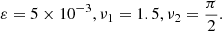
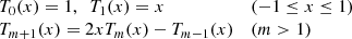
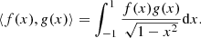
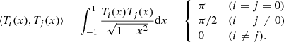
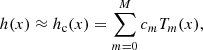
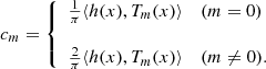
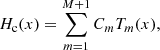
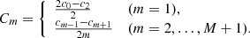
| Issue |
A&A
Volume 628, August 2019
|
|
|---|---|---|
| Article Number | A84 | |
| Number of page(s) | 13 | |
| Section | Numerical methods and codes | |
| DOI | https://doi.org/10.1051/0004-6361/201730492 | |
| Published online | 13 August 2019 | |
Frequency analysis and representation of slowly diffusing planetary solutions⋆
1
Purple Mountain Observatory, Chinese Academy of Sciences, 2 West Beijing Road, 210008 Nanjing, PR China
e-mail: This email address is being protected from spambots. You need JavaScript enabled to view it.
2
ASD/IMCCE, Observatoire de Paris, PSL University, CNRS, Sorbonne Université, 77 avenue Denfert-Rochereau, 75014 Paris, France
e-mail: This email address is being protected from spambots. You need JavaScript enabled to view it.
Received:
24
January
2017
Accepted:
10
January
2019
Abstract
Context. Over short time-intervals, planetary ephemerides have traditionally been represented in analytical form as finite sums of periodic terms or sums of Poisson terms that are periodic terms with polynomial amplitudes. This representation is not well adapted for the evolution of planetary orbits in the solar system over million of years which present drifts in their main frequencies as a result of the chaotic nature of their dynamics.
Aims. We aim to develop a numerical algorithm for slowly diffusing solutions of a perturbed integrable Hamiltonian system that will apply for the representation of chaotic planetary motions with varying frequencies.
Methods. By simple analytical considerations, we first argue that it is possible to exactly recover a single varying frequency. Then, a function basis involving time-dependent fundamental frequencies is formulated in a semi-analytical way. Finally, starting from a numerical solution, a recursive algorithm is used to numerically decompose the solution into the significant elements of the function basis.
Results. Simple examples show that this algorithm can be used to give compact representations of different types of slowly diffusing solutions. As a test example, we show that this algorithm can be successfully applied to obtain a very compact approximation of the La2004 solution of the orbital motion of the Earth over 40 Myr ([−35 Myr, 5 Myr]). This example was chosen because this solution is widely used in the reconstruction of the past climates.
Key words: methods: numerical / celestial mechanics / ephemerides / planets and satellites: dynamical evolution and stability / chaos
Full Tables A.3 and A.4 are only available at the CDS via anonymous ftp to cdsarc.u-strasbg.fr (130.79.128.5) or via http://cdsarc.u-strasbg.fr/viz-bin/qcat?J/A+A/628/A84
© Y. N. Fu and J. Laskar 2019
 Open Access article, published by EDP Sciences, under the terms of the Creative Commons Attribution License (http://creativecommons.org/licenses/by/4.0), which permits unrestricted use, distribution, and reproduction in any medium, provided the original work is properly cited.
1. Introduction
Before the computer age, long-term solutions for planetary orbits were derived by perturbation methods, and were obtained in the form of the sum of periodic terms. The first such solution was obtained by Lagrange (1782) and was later on improved by LeVerrier (1840, 1841), who took Uranus into account as well. These long-term solutions have been found to be of fundamental importance for the understanding of the past climate of the Earth, when it was understood that the changes of the orbit of the Earth also induce some change in its obliquity and in the insolation at the Earth surface (Milankovitch 1941; for a detailed review, see Laskar et al. 2004). With the advent of computers, two different approaches become possible. Computer algebra allowed extending the perturbation methods (e.g., Bretagnon 1974), and as computer speed increased, direct integrations of the full solar system become possible (Quinn et al. 1991; Sussman & Wisdom 1992). Instead, Laskar (1985, 1986, 1988) developed a mixed strategy in which an analytical averaging of the planetary equations by perturbation methods was obtained with dedicated computer algebra, followed by numerical integration of the averaged system. In order to compare the output of the numerical integrations with the quasi-periodic solutions of the perturbative methods, Laskar (1988) introduced the frequency analysis method that allows obtaining in a very efficient way a precise approximation of the numerical solution in quasiperiodic form (e.g., Laskar 2003).
One outcome of these computations was also to demonstrate that the solar system motion is chaotic (Laskar 1989, 1990). As a consequence, the solutions are not quasi-periodic, although they can be approximated by a quasi-periodic expression over a limited time of a few million years (Laskar 1988, 1990; Laskar et al. 2004).
We here derive a more adapted strategy for the slowly diffusing trajectories of a dynamical system that is very well suited to the construction of compact forms for the long-time behavior of planetary orbits. We introduce an algorithm that is derived from the frequency analysis to which a slow variation of the frequencies and amplitudes is added. By slowly diffusing solution, we mean a solution that while it experiences significant frequency drifts during the entire considered time interval is nearly quasi-periodic in time subintervals. Similar to the frequency analysis, a key step of our algorithm is to construct a frequency-dependent function basis on which the considered solution is decomposed.
After recalling some fundamental results of the frequency analysis, we consider in Sect. 2 a single-term model and show that it is possible to exactly recover its varying frequency as a function of time. This is important when the details of how a solution diffuses in the frequency space are of interest. To construct a compact solution representation with a reasonably high precision, however, small flickers without significant cumulative effects can be smoothed out from a varying frequency. It is therefore preferable to use a model with a limited number of parameters, for instance, low-order polynomials, to approximate the frequency. To do so, we sample the averaged frequencies over a sliding time-interval. For a slowly diffusing solution, it is assumed that all fundamental frequencies can be sampled in this way using the algorithm called numerical analysis of fundamental frequencies (NAFF; e.g., Laskar 2003).
We design a general algorithm that represents a slowly diffusing solution in Sect. 3, where a frequency-dependent function basis is constructed based on the Chebyshev approximations of fundamental frequencies. The basis functions with significant but non-fundamental frequencies are generated according to the assumption that at any instant, a slowly diffusing solution is nearly quasi-periodic with the smoothed fundamental frequencies at that instant: all main frequencies are integral linear combinations of the fundamental frequencies. This effectively avoids the difficulties of determining the frequencies of long-period terms and/or groups of neighboring-period terms.
Two simple examples are given in Sect. 4. In the first example, a weakly dissipated system is considered, and the represented solution diffuses because of dissipation. In the second example, a Hamiltonian system of degree 1.5 is considered, and a solution starting from an obvious resonance overlap zone is represented. To show the flexibility of our algorithm in representing such a solution, we exclude all possible libration frequencies from the set of fundamental frequencies used in constructing the function basis.
Applications to the representation of ephemerides of the solar system bodies are provided in Sect. 5. As examples, we represent the eccentricity and inclination of the Earth as given by the long-term numerical solution La2004 (Laskar et al. 2004). For such a realistic solution, it is natural to take restrictions on the representation model from previous results into account, such as the important libration frequencies from numerical analysis (e.g., Laskar et al. 2004), so that the resulting representations can be as similar as possible to the physical model.
2. Frequency analysis and time-dependent frequencies
For a KAM solution (after Kolmogorov, Arnold, Moser) of a dynamical system (Kolmogorov 1954; Arnol’d 1963; Moser 1962), with fundamental frequency vector ν = (ν1, …, νN)∈RN, where N is the number of degrees of freedom of the system, the motion of any given degree of freedom variable z(t) can be described in complex form as
 (1)
(1)
where k = (k1, …, kN) is the frequency index vector, ak complex amplitude, and ⟨ ⋅ , ⋅ ⟩ denotes the usual inner product of two real vectors.
The NAFF algorithm was designed to numerically recover significant terms of Eq. (1) from a numerical sample set of z(t), for example, an ephemeris obtained by numerical integration (Laskar 1988). However, the application of NAFF is not limited to numerically recovering KAM solutions. Actually, most of the relevant works concern frequency drifts. In particular, the variations in fundamental frequencies of the secular solar system over 200 Myr was used to study the chaotic behavior of the solar system (Laskar 1990).
We first briefly recall the theorem about the convergence of the NAFF algorithm (for the complete version with proof, see Laskar 2003). With a set of N appropriate variables, the complex function (1) describing a degree of freedom of an analytic KAM solution can be written as
 (2)
(2)
where ν1 is a fundamental frequency. We have then the following (e.g. Laskar 1999).
Theorem 1. Let  be the value of σ ∈ R that maximizes the function
  , where χ = χ(t/T) > 0 is a weight function, and
  the inner product of two complex functions of t defined as
 (3)
(3)
We then have  .
.
Similar to the fundamental frequency ν1, any other main frequency can be recovered by searching its neighborhood or R for the value of σ that maximizes ϕ(σ), defined with the remaining z(t), that is, the original z(t) minus the recovered terms.
A diffusion solution is then characterized by fundamental frequency variations (Laskar et al. 1992; Laskar 1993). To determine a varying frequency, we first consider the following simplest case,
 (4)
(4)
where ν(t) and a(t) > 0 are real integrable functions. Writing
 (5)
(5)
where  belongs to 𝒞0, the set of continuous function on R, we have the theorem below.
Theorem 2. For any given T > 0 and ν(t)∈𝒞0, the functional ϕ(σ(t)) has one and only one maximum in 𝒞0, which is attained at σ(t)≡ν(t).
Proof. The right-hand side of Eq. (5) can be written as

Using the Cauchy–Bunyakovsky–Schwarz inequality1, we can easily deduce from this formula that

where ∥ ⋅ ∥ denotes the norm induced by the inner product (3). Moreover, the equality is true if and only if  and
and  are linearly dependent, that is, when θ(t) is a constant. This constant is 0, since θ(0)=0 by definition. The above arguments imply that ϕ(σ(t)) has a unique maximum attained at θ(t)≡0. Because ν(t) is continuous and the searched σ(t) is also continuous, θ(t)≡0 is equivalent to σ(t)≡ν(t). We therefore conclude for any given T > 0 that ϕ(σ(t)) has one and only one maximum attained at σ(t)≡ν(t) ▫.
Theorem 2 implies that even in the case of a varying frequency, it is still possible to recover the frequency exactly, as a function of time. Now, we consider the following more general complex function:
 (6)
(6)
where a1(ak)∈Sa with Sa a subspace of real function space, θk ∈ R, and  with Sν a linear subspace of the real integrable function space. As an extension of Eq. (2), this function inherits an important time-varying character of Eq. (2), that is, all phase increments are described by a single fundamental frequency vector ν(t). We make the heuristic assumption that under suitable conditions, a similar result as for Theorem 1 holds for a more general expression with varying frequencies as in Eq. (6).
Assumption. If  is sufficiently small, where
  and ∥ ⋅ ∥ is an appropriately defined T-dependent norm (e.g., the one induced by the inner product (3)), and
  (locally) maximizes the functional
  , then
  .
.
3. Representation of slowly diffusing solutions
From now on, we restrict ourselves to slowly diffusing solutions of an ordinary differential equation system obtained by slightly perturbing an integrable Hamiltonian system. We denote by  the action-angle variables of the integrable Hamiltonian system, which is used to express the ephemeris of a diffusing solution
  .
.
3.1. Representation procedure
We start from a sample set of  . We assume that the samples are given at grid points from t0 to t1 with fixed time step h, which is much smaller than the minimum of the fundamental periods. In accordance with the condition of slow diffusion, we assume that the solution is close to quasi-periodic in the time subintervals (of [t0, t1]) described below, with a length far exceeding the maximum of the fundamental periods. These roughly stated preconditions are required because we use NAFF algorithm to estimate the changing fundamental frequencies.
As the first step, we apply the NAFF algorithm to obtain fundamental frequency samples. For each given degree (n), this algorithm is applied to zn(t) samples over evenly spaced time-subintervals ![Mathematical equation: $ \{[\tau_\lambda-\frac{d}{2},\tau_\lambda+\frac{d}{2}]\}_{\lambda=1}^{\Lambda} $](/articles/aa/full_html/2019/08/aa30492-17/aa30492-17-eq25.gif) of
of ![Mathematical equation: $ [t_0,t_1]=[\tau_1-\frac{d}{2},\tau_\Lambda+\frac{d}{2}] $](/articles/aa/full_html/2019/08/aa30492-17/aa30492-17-eq26.gif) . For each of these subintervals, the first recovered frequency is taken as the averaged value of the fundamental frequency νn over the same subinterval. The N averaged fundamental frequencies obtained in this way are then taken as the instant frequencies at τλ, resulting in the fundamental frequency samples
. For each of these subintervals, the first recovered frequency is taken as the averaged value of the fundamental frequency νn over the same subinterval. The N averaged fundamental frequencies obtained in this way are then taken as the instant frequencies at τλ, resulting in the fundamental frequency samples 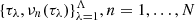 .
.
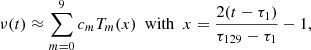
Second, we fit for each given degree the frequency samples to a Chebyshev expansion valid on [τ1, τΛ],
 (7)
(7)
where cm, n ∈ R is a Chebyshev coefficient, ![Mathematical equation: $ x=\frac{2(t-\tau_1)}{(\tau_{\Lambda}-\tau_1)}-1 \in [-1,1] $](/articles/aa/full_html/2019/08/aa30492-17/aa30492-17-eq29.gif) a normalized time, and Tm(x) is the Chebyshev polynomial2 of degree m. We then numerically construct a frequency-dependent function basis B (see the next subsection), on which the considered solution is decomposed.
a normalized time, and Tm(x) is the Chebyshev polynomial2 of degree m. We then numerically construct a frequency-dependent function basis B (see the next subsection), on which the considered solution is decomposed.
The final step, that is, decomposing zn(t) on B, is the same as that of the NAFF algorithm (Laskar 1999), except for the searched function bases for significant terms. The function bases are {eiωkt, ωk ∈ R} for NAFF and B for the procedure described here.
3.2. Representation model
By variation of parameters, Eq. (1) becomes
 (8)
(8)
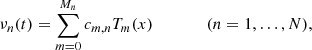
Now, let
 (9)
(9)
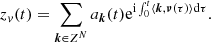
be a truncated set of the frequency index vector k. For each  , let
, let
 (10)
(10)
be a Chebyshev expansion of the amplitude valid on [τ1, τΛ], where  . These lead us from Eq. (8) to the following representation model of zv(t):
 (11)
(11)
From the Chebyshev approximations of the fundamental frequencies, it is easy to obtain by integration the Chebyshev expansion representing the phase increment associated with the frequency ⟨k, ν(τ)⟩, from the value, as is preferred, at the middle of the time interval [τ1, τΛ],
 (12)
(12)
where φ0k ∈ R, and φk(t) gathers all Chebyshev polynomials of degree larger than 0. With φ0k and φk(t), Eq. (11) can be written as
 (13)
(13)
where  is simply the coordinate of zv(t) when it is decomposed on the function basis
 (14)
(14)
For the obtained representation, it should be noted that although we decompose a solution on the basis B, and correspondingly, express its representation by Eq. (13), φk(t) is not used to specify the representation.  is used instead. In other words, the representation is specified by the coordinates al, k, and the Chebyshev coefficients of
  . This choice is made for the following two reasons. One is that the representation could otherwise be unnecessarily cumbersome. The other reason is that from the Chebyshev coefficients of
  , those of φk(t) can be easily obtained according to Eq. (12). Here, we also recall that the solution representation, because of its dependence on the Chebyshev approximations of νn(t) and ak(t), is valid on [τ1, τΛ] rather than [t0, t1].
To complete the description of the representation model, we point out that the integers  and
and  , introduced in Eqs. (7), (9), and (10), respectively, are necessary parameters for defining a particular representation procedure. Of course, the number of these parameters can be reduced by requiring that some or all of these parameters take the same sufficiently high value, for instance, Lk = L for all
  , at the price of unnecessarily increasing the basis dimension. Another important point to mention is that to terminate the procedure, the maximum number of representation terms (J) and/or the required precision has to be set beforehand. The required precision is specified by using either the absolute truncation error δ or the relative truncation error δr. Correspondingly, the procedure is terminated if
 (15)
(15)
or
 (16)
(16)
where the module ∥ ⋅ ∥ is induced by the inner product (3) with prescribed χ ≡ 1. In the following, these parameters, as summarized in Table 1, are referred to as procedure parameters.
Summary of procedure parameters.
4. Examples
In the following two subsections, we illustrate our representation procedure with two slowly diffusing solutions, of which one diffuses as a result of a dissipative perturbation, and the other as a result of its chaotic nature. In order to illustrate the convergence property of this procedure, it is convenient to write the resulting representation with a single term index, that is,
 (17)
(17)
where the terms are arranged in the same order as they are obtained in the procedure, which roughly corresponds to the order of decreasing |aj|.
4.1. Example of a dissipated solution
Consider the following weakly dissipated system:
 (18)
(18)
where
 (19)
(19)
If we nullify the dissipative term  in Eq. (18), the system is a simple pendulum with Hamiltonian
 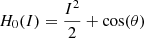 , where
  . Take as an example the solution z(t)≡I(t)ei θ(t) of Eq. (18) with the following initial conditions:
 (20)
(20)
Because of the dissipative perturbation, the phase orbit starting from (θ0, I0) gradually decays away from the unperturbed orbit passing through the same phase point. This dissipation effect is significant in the long run, as is shown in Fig. 1.
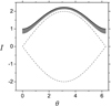 |
Fig. 1. Phase trajectory of the dissipated solution specified by Eqs. (18)–(20). Also shown is the phase orbit of the unperturbed pendulum system, namely (Eq. (18)) with ε = 0, which passes through the initial phase point of the dissipated solution. The dashed line depicts the separatrix of the unperturbed pendulum. |
As a solution of a system of 1 degree of freedom with a dissipative perturbation, the decaying z(t) has a changing fundamental frequency ν, which inherits the characteristic frequency of the unperturbed system and varies as the solution decays.
4.2. Practical implementation
By numerical integration, an ephemeris of z(t) is obtained at {ti = ih : i = 0, …, 65535, h = 0.15}. We then apply NAFF to 129 evenly spaced time subintervals with length d = 2048 h and midpoints 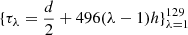 , respectively, to obtain a sample set of the changing frequency,
  . This frequency sample set is shown in Fig. 2. We also show a Chebyshev expansion approximating ν(t). This expansion is of degree 9 and is expressed as
 (21)
(21)
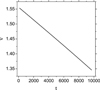 |
Fig. 2. Change of the fundamental frequency ν(t) of the dissipated solution specified by Eqs. (18)–(20). Also shown is a Chebyshev approximation of ν(t). |
where the Chebyshev polynomials Tm(x) are listed in Table A.1 and x is the time after normalization from [τ1, τ129] to [ − 1, 1]. The values of the coefficients  are given in Table 2.
We write the Chebyshev expansion approximating the phase increment, from the value at x = 0 or  , associated with ν in two parts,
 (22)
(22)
where φ0 is a real constant and
 (23)
(23)
gathers all Chebyshev polynomials of degree larger than 0. In Eq. (23),  is the time-scaling factor, and3, with c10 = c11 = 0,
 (24)
(24)
This completes the determination of φ(x), which is used in the following. Although the constant φ0 is not used in the following, it can be easily determined as φ0 = −φ(0) because the phase increment (22) is 0 at  or x = 0.
With procedure parameters {M, K, L, δr} = {9, 10, 9, 10−5}, we obtain a 37-term representation,
 (25)
(25)
of the solution z(t), where Tl(j)(x) is the Chebyshev polynomial of degree l(j), and φk(j)(x)=k(j)φ(x) the phase increment associated with the frequency k(j)ν. The data needed for specifying the first ten representation terms are given in Table 3.
We now discuss how the procedure parameters affect the precision of the resulting representation. For this, we first consider a 150-term representation obtained by resetting M = 1. This resetting introduces only a small discrepancy in ν(t) because |cm/c0|< 6 × 10⁻⁴ for m > 1. The precision of this representation is several orders less precise than the previous one. As seen by comparing the two panels of Fig. 3, this is because the whole considered time interval is long, and the small discrepancy in ν(t) can accordingly result in significant phase errors. On the other hand, however, the fact that there is no term with either |k|> 8 or l > 4 in the 37-term representation indicates that the representation model practically converges with respect to K and L. Our representation procedure also converges rapidly with respect to J. This is illustrated in Fig. 4, for which the procedure parameters excluding J are fixed as {M, K, L} = {9, 10, 9}.
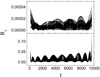 |
Fig. 3. Errors of two different representations of the dissipated solution specified by Eqs. (18)–(20). In the case of the upper panel, our representation procedure is terminated with a 37-term representation, because this representation reaches the precision requirement δr = 10−5. In the case of the lower panel, with slightly larger error in the frequency approximation, the representation is about 4 orders less precise, though the number of representation terms is increased to 150. |
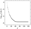 |
Fig. 4. Convergence property of the procedure of representing the dissipated solution specified by Eqs. (18)–(20). The residual of the representation is plotted against the number J of representation terms, where other procedure parameters are fixed as {M, K, L} = {9, 10, 9}. |
4.3. Example of chaotic solutions of Hamiltonian system
We consider the following Hamiltonian system:
![Mathematical equation: $$ \begin{aligned} H(I,\theta ,t)=\frac{I^2}{2} + \varepsilon \cos (\theta )[1+\cos (\nu _1 t)+\cos (\nu _2 t)], \end{aligned} $$](/articles/aa/full_html/2019/08/aa30492-17/aa30492-17-eq67.gif) (26)
(26)
where
 (27)
(27)
A solution of this system has three fundamental frequencies. The first two are the forcing frequencies ν1 and ν2, which are non-commensurable. The other, denoted as ν3, can be approximated in a similar way as in the previous subsection.
From the analysis of the frequency map (e.g., Laskar 1999), defined as I0 → ν3 with θ0 = 0 and shown in Fig. 5, we know that the phase point
 (28)
(28)
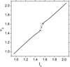 |
Fig. 5. Fundamental frequency map of the system specified by Eqs. (26) and (27). In the chaotic zone formed by resonance overlap lies the phase point (θ0, I0) = (0, 1.535), which will be chosen as the initial phase point of the considered chaotic solution. |
lies in a chaotic zone formed by resonance overlap, and the solution z(t) starting from this point is chaotic.
An ephemeris of z(t) is obtained by the symplectic integrator SBABc4 (Laskar & Robutel 2001) at {ti = ih : i = 0, …, 4095, h = 0.186058}. We then apply NAFF to 129 evenly spaced time intervals with length d = 512 h and midpoints 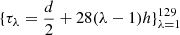 . This gives the sample set
  , partly shown in Fig. 6 together with a Chebyshev approximation. It should be noted that there are two intrinsically different error sources in this way of approximating a changing frequency. One error source is related to the NAFF process that gives the samples of the frequency, while the other is related to the fitting process that leads to a Chebyshev approximation of the frequency. Accordingly, we consider the Chebyshev approximation as sufficiently good if it deviates from the frequency sample set by much less than the sample uncertainties. As shown in Fig. 6, this requirement can be met with a Chebyshev polynomial of degree M3 = 9.
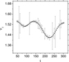 |
Fig. 6. Change of fundamental frequency ν3(t) of the chaotic solution specified by Eqs. (26)–(28). The samples of this frequency are computed by applying NAFF algorithm over a sliding time-interval, and the errors are estimated as their respective differences from the frequencies of the quasi-periodic approximation of the solution over the same sliding time interval. Also shown is a Chebyshev appoximation of ν3(t). |
Test calculations show that our representation procedure cannot lead to an acceptable representation of the solution on the whole sampling time-interval. There are two possible reasons for this.
The most intrinsic reason would be that our solution experiences passages into or out of resonance zones. Such a passage is associated with a shift between circulation and libration of the corresponding resonance angle, and accordingly, with occurrence or disappearance of certain terms. If some of these terms are significant enough in the whole considered time interval (τ1, τ129), then there would be no way to obtain any acceptable non-piecewise representation. Therefore, we restrict ourselves to the shorter time interval (τ1, τ50).
Another possible reason is that there are one or more significant libration frequencies, which are not taken into consideration when we generate the function basis B. While it is easy to make a necessary extension of B in order to include known libration frequencies (see Sect. 5), it is not that straightforward to identify and sample these frequencies (Laskar 1990). To show the flexibility of our algorithm, we do not search for any libration frequency and make the corresponding extension of B. The flexibility arises because when we choose reasonably high values of our procedure parameters Kn, then the resulting set of frequencies would be dense enough over a large frequency interval, in the sense that every important libration frequency is not far from at least one element of the frequency set.
Setting the procedure parameters as

we obtain a 100-term representation of our solution. Figure 7 shows that the errors of this representation are typically smaller than 10−4I0. Figure 8 also illustrates, in the same way as in the previous subsection, the convergence property of the representation procedure.
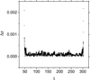 |
Fig. 7. Error of a 100-term representation of the chaotic solution specified by Eqs. (26)–(28). This representation is obtained with {M1, M2, M3, K1, K2, K3, Lk, J} = {0, 0, 9, 10, 10, 10, 9, 100}. |
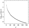 |
Fig. 8. Convergence property of the procedure of representing the chaotic solution specified by Eqs. (26)–(28). The residual of representation is plotted against the number J of representation terms. The other procedure parameters are fixed as {M1, M2, M3, K1, K2, K3, Lk} = {0, 0, 9, 10, 10, 10, 9}. |
5. Application to planetary ephemerides
Numerical integration is now an efficient way of constructing ephemerides of the solar system bodies with high precision. For practical applications, however, it can be useful to represent these discrete solutions analytically, and thus represent them in a continuous way.
These representations can be made in the form of segmented Chebyshev expansions, like those that represent the classical planetary ephemerides as INPOP (e.g., Fienga et al. 2008), or other generally applied approximation models without physical basis. A drawback of these representations is that they require large amounts of data. In order to obtain compact representations, Chapront (1995) used a model of Poisson series with fixed main frequencies that were obtained with the NAFF algorithm. Although this model already involves some long-term or long-period-term effects by allowing Poisson terms and therefore works well with planetary ephemerides of five outer planets over a few hundred years, it does not take the frequency drifts into consideration and cannot be used over millions of years.
The frequency drifts are important over a few tens of million years, as shown by Laskar (1990). The algorithm developed here is therefore expected to be more appropriate in representing ephemerides spanning this long time-interval. It is thus interesting to test whether our algorithm can be used to represent the long-term numerical solution of major solar system bodies over this long timescale (e.g., Laskar et al. 2004). For this, we applied our algorithm to the eccentricity and inclination variables of the Earth, that is,
 (29)
(29)
To be more precise, e3 and i3 are the eccentricity and inclination, respectively, of the instantaneous orbit of the Earth-Moon barycenter, and ϖ3 and Ω3 are the longitudes of the perihelion and of the node of the same orbit with respect to the fixed J2000.0 equatorial reference system, respectively.
The chaotic behavior of the terrestrial orbit certainly limits the time span over which this orbit can be precisely determined, but z3 and ζ3 from La2004 are reliable and precise at least over the time span [−35 Myr, +5 Myr], see Laskar et al. (2011). Therefore, we restricted our representations to this time span. Test calculations showed that our algorithm can lead to compact and precise representations for both degrees of freedom. With different procedure parameters, the resulting representations contain very different terms. This confirms the flexibility of our algorithm.
In order to give representations as physical as possible, we resorted to the knowledge we have for the solution. Following Laskar et al. (2004), we computed the fundamental frequencies of the secular solar system by applying the NAFF algorithm over time intervals of length 20 Myr for the proper modes  , and 50 Myr for the proper modes
  4. From −35 Myr to 5 Myr with a step 0.1 Myr, we generated the samples of the fundamental frequencies (g1, …, g8, s1, …, s8) corresponding to these proper modes. The resulting nominal value of s5 is about 0.00000015 arcsec yr−1. The other frequency samples are shown in the panels of Fig. 9, where the errors are estimated as the difference between the values of a frequency computed from the associated ephemeris and its quasi-periodic approximation. We also show in this figure the Chebyshev approximations of these fundamental frequencies. All of these Chebyshev approximations, the coefficients of which are listed in Table A.2, were obtained by truncating those of degree 15. The truncation criterion was roughly that the discrepancy in a fundamental frequency should not induce an error in phase larger than 2π/104 over several tens of million years.
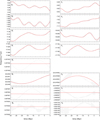 |
Fig. 9. Variations of major fundamental frequencies of the solar system over the time interval from −35 Myr to 5 Myr with origin at J2000. These frequencies (in arcsec yr−1) are computed by applying the NAFF algorithm to the proper modes of the secular solar system associated with major planets. The errors in the resulting frequency samples are estimated as the difference between the frequencies computed respectively from the original ephemeris and its quasi-periodic approximation. Also shown in this figure are the Chebyshev approximations of these varing fundamental frequencies (red curves), which are specified in Table A.2. |
There are two important libration frequencies, r1 = 0.251085 arcsec yr−1 of the resonance argument  and r2 = 0.117222 arcsec yr−1 of
  . To include them as additional fundamental frequencies, we expressed the main frequency as
 (30)
(30)
The d’Alembert characteristic, 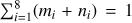 , was used to exclude non-physical frequency index vectors.
To show to which degree our algorithm is practically useful, we discuss here the following two 100-term representations (ℜ100 for short),
 (31)
(31)
where with f = (g1, …, g8, s1, …, s8, r1, r2) and k = (m1, …, m8, n1, …, n8, k1, k2), the phase increment  is associated with the main frequency ⟨k, f⟩. The way the residuals decrease with increasing number of representation terms in the two representation procedures of ℜ100 is shown in Fig. 10.
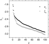 |
Fig. 10. Convergence property of the two representation procedures leading to the 100-term representations of z3(t) and ζ3(t). The residual of the representation is plotted against the number J of the representation terms. |
The leading 40 terms of these two representations are given in Tables A.3 and A.4, respectively, where the terms are reordered according to their real amplitudes and data are rounded to a convenient number of digits. Comparing these results with those given in Tables 4 and 5 of Laskar (1990), we find that they are coherent with each other in the sense that all the main frequencies explicitly identified previously can be found in our tables.
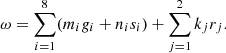
The full versions of Tables A.3 and A.4 are available at the CDS. They are plain-text tables providing all terms of ℜ100 in the form of Eq. (31). Together with the data presented in Table A.2 for computing f, these two tables can be used to compute the eccentricity and inclination variables from ℜ100. The errors of ℜ100 as solution representation are shown in Fig. 11. Based on the information in this figure, we expect that our algorithm should be efficient in producing compact and precise representations of long-term ephemerides of major solar system bodies.
 |
Fig. 11. Comparison between the eccentricity and inclination ephemerides of La2004 and their respective 100-term representations over the time interval from −35 Myr to 5 Myr with origin at J2000. Both representations are in the form of Eq. (31), with the Chebyshev expansions approximating the fundamental frequencies specified in Table A.2, and main frequency index vectors and complex amplitudes of all 100 terms in the full Tables A.3 and A.4 available at the CDS. |
To conclude, we explicitly illustrated the advantage of representing ephemerides by taking into consideration the frequency drifts by comparing the representations given by a direct use of NAFF and the modified present algorithms. The quasi-periodic representations (ℜNAFF for short) of the same z3- and ζ3-ephemeris given by the standard realization of NAFF, which is a built-in tool of the algebraic system TRIP5, have 50 and 41 terms, respectively. NAFF does not recover more terms because it encounters a frequency that at a given level of precision is already recovered in a previous step. To more precisely show the advantage of taking frequency drifts into consideration, we produced for z3 and ζ3 representations (ℜ) with the same number of terms as the corresponding ℜNAFF representation. The comparison between ℜ and ℜNAFF is shown in Fig. 12. This figure clearly shows the improvements brought by introducing frequency drifts into the representation model.
 |
Fig. 12. Comparison between the eccentricity ephemeris z3 and the inclination ephemeris ζ3 of La2004 and their respective representations by NAFF (ℜNAFF) and by the present algorithms (ℜ). The number of terms of z3-representation is 50 for both ℜNAFF and ℜ, and the number is 41 in the case of ζ3. |
Given any two vectors f and g in an inner product space, the Cauchy–Bunyakovsky–Schwarz inequality writes ⟨f, g⟩≤∥f∥×∥g∥, where ⟨ ⋅ , ⋅ ⟩ denotes the inner product and ∥ ⋅ ∥ the induced norm. In addition, the equality is true if and only if f and g are linearly dependent.
The explicit expressions of Tm(x) up to m = 15 are given in Table A.1.
For the general case, see Eq. (A.7).
See Laskar (1990) for the definition of the proper modes.
Acknowledgments
P. Robutel and L. Niederman are thanked for their time in instructive discussions, and M. Gastineau for various kinds of helps. Fu is indebted to many colleagues from IMCCE for their hospitality. Fu is supported by NSFC grants No. 11178006-11273066-11533004.
References
- Arnol’d, V. I. 1963, Russ. Math. Surv., 18, 9 [Google Scholar]
- Bretagnon, P. 1974, A&A, 30, 141 [NASA ADS] [Google Scholar]
- Chapront, J. 1995, A&AS, 109, 181 [NASA ADS] [Google Scholar]
- Fienga, A., Manche, H., Laskar, J., & Gastineau, M. 2008, A&A, 477, 315 [NASA ADS] [CrossRef] [EDP Sciences] [Google Scholar]
- Kolmogorov, A. 1954, Dokl. Akad. Nauk. SSSR, 98, 469 [Google Scholar]
- Lagrange, J. L. 1782, Oeuvres Complètes, 5, 211 [Google Scholar]
- Laskar, J. 1985, A&A, 144, 133 [NASA ADS] [Google Scholar]
- Laskar, J. 1986, A&A, 157, 59 [NASA ADS] [Google Scholar]
- Laskar, J. 1988, A&A, 198, 341 [NASA ADS] [Google Scholar]
- Laskar, J. 1989, Nature, 338, 237 [NASA ADS] [CrossRef] [Google Scholar]
- Laskar, J. 1990, Icarus, 88, 266 [NASA ADS] [CrossRef] [Google Scholar]
- Laskar, J. 1993, Phys. D, 67, 257 [Google Scholar]
- Laskar, J. 1999, Hamiltonian Systems with Three or More Degrees of Freedom, 134 [CrossRef] [Google Scholar]
- Laskar, J. 2003, ArXiv e-prints [arXiv:math/0305364] [Google Scholar]
- Laskar, J., & Robutel, P. 2001, Celestial Mech. Dyn. Astron., 80, 39 [NASA ADS] [CrossRef] [Google Scholar]
- Laskar, J., Froeschlé, C., & Celletti, A. 1992, Phys. D Nonlinear Phenom., 56, 253 [CrossRef] [Google Scholar]
- Laskar, J., Robutel, P., Joutel, F., et al. 2004, A&A, 428, 261 [NASA ADS] [CrossRef] [EDP Sciences] [Google Scholar]
- Laskar, J., Fienga, A., Gastineau, M., & Manche, H. 2011, A&A, 532, A89 [NASA ADS] [CrossRef] [EDP Sciences] [Google Scholar]
- LeVerrier, U. 1840, Additions à la Connaissance des temps pour l’an 1843 (Paris: Bachelier), 3 [Google Scholar]
- LeVerrier, U. 1841, Additions à la Connaissance des temps pour l’an 1843 (Paris: Bachelier), 28 [Google Scholar]
- Milankovitch, M. 1941, Kanon der Erdbestrahlung und seine Anwendung auf das Eiszeitenproblem (Belgrade: Spec. Acad. R Serbe) [Google Scholar]
- Moser, J. K. 1962, Nach. Akad. Wiss. Göttingen, Math. Phys., II, 1 [Google Scholar]
- Quinn, T. R., Tremaine, S., & Duncan, M. 1991, ApJ, 101, 2287 [Google Scholar]
- Sussman, G. J., & Wisdom, J. 1992, Science, 257, 56 [NASA ADS] [CrossRef] [PubMed] [Google Scholar]
Appendix A: Chebyshev polynomials and coefficients for the La2004 solution
Expressions of the Chebyshev polynomials up to degree 15.
A.1. Chebyshev polynomials
Chebyshev polynomials as defined by the recurrence relation
 (A.1)
(A.1)
form a non-normalized but orthogonal basis under the inner product
 (A.2)
(A.2)
This can be easily checked by straightforward calculations
 (A.3)
(A.3)
Their linear combination, called Chebyshev expansion, is often used to approximate a function h(x) defined on [ − 1, 1]
 (A.4)
(A.4)
where
 (A.5)
(A.5)
The indefinite integral of the Chebyshev expansion hc(x) writes, up to an arbitrary constant,
 (A.6)
(A.6)
where, with cM + 1 = cM + 2 = 0,
 (A.7)
(A.7)
A.2. Coefficients for the Earth La2004 solution
Here we provide the tables of coefficients used for the representation of the Earth La2004 eccentricity and inclination solution over the interval [−35 Myr: +5 Myr] (Laskar et al. 2004).
Coefficients of Chebyshev expansion ∑mcmTm approximating the major fundamental frequencies (g1, …, g8, s1, …, s8) (arcsec yr−1) of the solar system over the time interval from −35 Myr to 5 Myr with origin at J2000.
Leading 40 terms of the 100-term representation z3(t), as expressed in Eq. (31).
Leading 40 terms of the 100-term representation ζ3(t), as expressed in Eq. (31).
All Tables
Coefficients of Chebyshev expansion ∑mcmTm approximating the major fundamental frequencies (g1, …, g8, s1, …, s8) (arcsec yr−1) of the solar system over the time interval from −35 Myr to 5 Myr with origin at J2000.
Leading 40 terms of the 100-term representation z3(t), as expressed in Eq. (31).
Leading 40 terms of the 100-term representation ζ3(t), as expressed in Eq. (31).
All Figures
|
Fig. 1. Phase trajectory of the dissipated solution specified by Eqs. (18)–(20). Also shown is the phase orbit of the unperturbed pendulum system, namely (Eq. (18)) with ε = 0, which passes through the initial phase point of the dissipated solution. The dashed line depicts the separatrix of the unperturbed pendulum. |
| In the text | |
|
Fig. 2. Change of the fundamental frequency ν(t) of the dissipated solution specified by Eqs. (18)–(20). Also shown is a Chebyshev approximation of ν(t). |
| In the text | |
|
Fig. 3. Errors of two different representations of the dissipated solution specified by Eqs. (18)–(20). In the case of the upper panel, our representation procedure is terminated with a 37-term representation, because this representation reaches the precision requirement δr = 10−5. In the case of the lower panel, with slightly larger error in the frequency approximation, the representation is about 4 orders less precise, though the number of representation terms is increased to 150. |
| In the text | |
|
Fig. 4. Convergence property of the procedure of representing the dissipated solution specified by Eqs. (18)–(20). The residual of the representation is plotted against the number J of representation terms, where other procedure parameters are fixed as {M, K, L} = {9, 10, 9}. |
| In the text | |
|
Fig. 5. Fundamental frequency map of the system specified by Eqs. (26) and (27). In the chaotic zone formed by resonance overlap lies the phase point (θ0, I0) = (0, 1.535), which will be chosen as the initial phase point of the considered chaotic solution. |
| In the text | |
|
Fig. 6. Change of fundamental frequency ν3(t) of the chaotic solution specified by Eqs. (26)–(28). The samples of this frequency are computed by applying NAFF algorithm over a sliding time-interval, and the errors are estimated as their respective differences from the frequencies of the quasi-periodic approximation of the solution over the same sliding time interval. Also shown is a Chebyshev appoximation of ν3(t). |
| In the text | |
|
Fig. 7. Error of a 100-term representation of the chaotic solution specified by Eqs. (26)–(28). This representation is obtained with {M1, M2, M3, K1, K2, K3, Lk, J} = {0, 0, 9, 10, 10, 10, 9, 100}. |
| In the text | |
|
Fig. 8. Convergence property of the procedure of representing the chaotic solution specified by Eqs. (26)–(28). The residual of representation is plotted against the number J of representation terms. The other procedure parameters are fixed as {M1, M2, M3, K1, K2, K3, Lk} = {0, 0, 9, 10, 10, 10, 9}. |
| In the text | |
|
Fig. 9. Variations of major fundamental frequencies of the solar system over the time interval from −35 Myr to 5 Myr with origin at J2000. These frequencies (in arcsec yr−1) are computed by applying the NAFF algorithm to the proper modes of the secular solar system associated with major planets. The errors in the resulting frequency samples are estimated as the difference between the frequencies computed respectively from the original ephemeris and its quasi-periodic approximation. Also shown in this figure are the Chebyshev approximations of these varing fundamental frequencies (red curves), which are specified in Table A.2. |
| In the text | |
|
Fig. 10. Convergence property of the two representation procedures leading to the 100-term representations of z3(t) and ζ3(t). The residual of the representation is plotted against the number J of the representation terms. |
| In the text | |
|
Fig. 11. Comparison between the eccentricity and inclination ephemerides of La2004 and their respective 100-term representations over the time interval from −35 Myr to 5 Myr with origin at J2000. Both representations are in the form of Eq. (31), with the Chebyshev expansions approximating the fundamental frequencies specified in Table A.2, and main frequency index vectors and complex amplitudes of all 100 terms in the full Tables A.3 and A.4 available at the CDS. |
| In the text | |
|
Fig. 12. Comparison between the eccentricity ephemeris z3 and the inclination ephemeris ζ3 of La2004 and their respective representations by NAFF (ℜNAFF) and by the present algorithms (ℜ). The number of terms of z3-representation is 50 for both ℜNAFF and ℜ, and the number is 41 in the case of ζ3. |
| In the text | |
Current usage metrics show cumulative count of Article Views (full-text article views including HTML views, PDF and ePub downloads, according to the available data) and Abstracts Views on Vision4Press platform.
Data correspond to usage on the plateform after 2015. The current usage metrics is available 48-96 hours after online publication and is updated daily on week days.
Initial download of the metrics may take a while.