| Issue |
A&A
Volume 627, July 2019
|
|
|---|---|---|
| Article Number | A111 | |
| Number of page(s) | 15 | |
| Section | The Sun | |
| DOI | https://doi.org/10.1051/0004-6361/201834702 | |
| Published online | 09 July 2019 | |
The evolution of coronal mass ejections in the inner heliosphere: Implementing the spheromak model with EUHFORIA
1
Catholic University of Leuven, Leuven, Belgium
e-mail: christine.verbeke@kuleuven.be
2
University of Helsinki, Helsinki, Finland
Received:
21
November
2018
Accepted:
17
March
2019
Aims. We introduce a new model for coronal mass ejections (CMEs) that has been implemented in the magnetohydrodynamics (MHD) inner heliosphere model EUHFORIA. Utilising a linear force-free spheromak (LFFS) solution, the model provides an intrinsic magnetic field structure for the CME. As a result, the new model has the potential to predict the magnetic components of CMEs at Earth. In this paper, we present the implementation of the new model and show the capability of the new model.
Methods. We present initial validation runs for the new magnetised CME model by considering the same set of events as used in the initial validation run of EUHFORIA that employed the Cone model. In particular, we have focused on modelling the CME that was responsible for creating the largest geomagnetic disturbance (Dst index). Two scenarios are discussed: one where a single magnetised CME is launched and another in which we launch all five Earth-directed CMEs that were observed during the considered time period. Four out of the five CMEs were modelled using the Cone model.
Results. In the first run, where the propagation of a single magnetized CME is considered, we find that the magnetic field components at Earth are well reproduced as compared to in-situ spacecraft data. Considering a virtual spacecraft that is separated approximately seven heliographic degrees from the position of Earth, we note that the centre of the magnetic cloud is missing Earth and a considerably larger magnetic field strength can be found when shifting to that location. For the second run, launching four Cone CMEs and one LFFS CME, we notice that the simulated magnetised CME is arriving at the same time as in the corresponding full Cone model run. We find that to achieve this, the speed of the CME needs to be reduced in order to compensate for the expansion of the CME due to the addition of the magnetic field inside the CME. The reduced initial speed of the CME and the added magnetic field structure give rise to a very similar propagation of the CME with approximately the same arrival time at 1 au. In contrast to the Cone model, however, the magnetised CME is able to predict the magnetic field components at Earth. However, due to the interaction between the Cone model CMEs and the magnetised CME, the magnetic field amplitude is significantly lower than for the run using a single magnetised CME.
Conclusions. We have presented the LFFS model that is able to simulate and predict the magnetic field components and the propagation of magnetised CMEs in the inner heliosphere and at Earth. We note that shifting towards a virtual spacecraft in the neighbourhood of Earth can give rise to much stronger magnetic field components. This gives the option of adding a grid of virtual spacecrafts to give a range of values for the magnetic field components.
Key words: magnetohydrodynamics (MHD) / methods: numerical / Sun: coronal mass ejections (CMEs) / Sun: magnetic fields / Sun: heliosphere / solar-terrestrial relations
© ESO 2019
1. Introduction
Coronal mass ejections (CMEs) are considered to be one of the main drivers of space weather (Gosling 1993; Huttunen et al. 2005; Hudson et al. 2006). They consist of large-scale eruptions of magnetised plasma, originating predominantly from active regions in the low solar corona and are extremely common events. During solar maxima, they occur on a daily basis, at times exceeding 10 events per day (Yashiro et al. 2004; Robbrecht et al. 2009; Webb & Howard 1994). CMEs can affect space missions and when they propagate towards Earth and interact with the magnetosphere, they can adversely impact a variety of assets, such as satellites, aviation, electricity networks and gas or oil pipelines. In addition, they can impact our daily life for example due to navigation system disturbances and failures (Schrijver et al. 2015, and references therein). Such impacts occur during geomagnetic storms and the prediction of such events and the level of impact on Earth that they incur is extremely important for our society. In daily operations when assessing the severity of a particular CME impact, two parameters in particular receive attention: the arrival time of the CME as well as the speed of the CME at arrival (Riley et al. 2018; Mays et al. 2015; Dumbović et al. 2018). However, while the speed as well as the density of the CME do impact the compression of the magnetosphere, it is nevertheless the magnetic structure of the ejecta that is mainly responsible for driving strong geomagnetic storms (Gonzalez et al. 1994; Lugaz et al. 2016; Kilpua et al. 2017).
For the past decade, in space weather operations, CMEs have mainly been modelled using the Cone model where the ejecta is treated as a hydrodynamic pulse that is characterized by a self-similar expanding geometry (Xie et al. 2004; Xue et al. 2005; Odstrčil & Pizzo 1999). As such the modelled CME does not contain an intrinsic magnetic field and only consists of a velocity, density and pressure enhancement that is injected at the inner radial boundary of the simulation domain that subsequently interacts with the background solar wind. One of the main physics-based models that has been operationally used by forecasting centres (see Riley et al. 2018 and the CME arrival time scoreboard1) such as the National Oceanic and Atmospheric Administration (NOAA) Space Weather Prediction Center (SWPC), the UK Met Office or the Royal Observatory of Belgium (ROB) Solar Influences Data Analysis Center (SIDC), is ENLIL (Odstrčil et al. 2004). While the model has certain advantages, such as the assumed geometry, the limited amount of input parameters and the robustness of the numerical algorithm due to more than a decade of use and fine-tuning, a significant limitation is the restriction of employing the Cone model with the result that the important north-south Bz component of the magnetic field is not accurately modelled. The most recent CME models focus on modelling the CME, not as a hydrodynamic pulse, but as a spheromak or exhibiting a toroidal-like flux rope structure such as SUSANOO-CME (Shiota & Kataoka 2016) and EEGGL+AWSoM_R (Sokolov et al. 2013; van der Holst et al. 2014; Jin et al. 2017).
In this work we present the new linear force-free spheromak (LFFS) model that has been implemented into the heliospheric magnetohydrodynamics (MHD) model EUHFORIA (EUropean Heliospheric FORecasting Information Asset, Pomoell & Poedts 2018). We focus in particular on addressing whether the LFFS model is capable of providing meaningful results for the observed magnetic Bz component. We aim to fully describe and detail the implementation and demonstrate its potential to simulate the magnetic field components at L1 (or any other position in the heliosphere). In future work, more in-depth parameter and case studies of the LFFS model will be presented in order to further study and exploit the predictive capabilities of the new CME model.
The paper is structured as follows. In Sect. 2, we briefly describe EUHFORIA and provide a detailed description of the implementation of the LFFS model. Section 3 contains a comparison of observational data and simulation results of the initial validation case considered in this paper. We discuss the results and future prospects in Sect. 4.
2. Numerical set-up
2.1. Modelling the solar background wind in the inner heliosphere
EUHFORIA is a newly developed three-dimensional magnetohydrodynamic (MHD) heliospheric model designed and used for space weather research as well as operational purposes (Pomoell & Poedts 2018). The model consists of two main parts: (1) a semi-empirical coronal model that aims to determine the solar wind plasma environment at the location of the inner boundary of the heliospheric model and (2) the heliospheric model that computes the dynamics in the inner heliosphere by numerically evolving the MHD equations. The work presented here has been obtained by using version 1.0.4.
The semi-empirical coronal model focuses on determining the solar wind plasma parameters at 0.1 au by using standard synoptic maps of the photospheric magnetic field observed by the Global Oscillation Network Group (GONG) of the National Solar Observatory (Harvey et al. 1996). First, the global three-dimensional coronal magnetic field in the lower corona is computed by employing a Potential Field Source Surface (PFSS) model (Altschuler & Newkirk 1969). Then, for the upper coronal domain, the Schatten Current Sheet (SCS) model is used to extend the model to 0.1 au (Schatten et al. 1969). The flux tube expansion factor f and the distance of the foot point of the flux tube to the nearest coronal hole boundary d, determined by employing the previously mentioned models, define the final solar wind speed νsw = ν(f, d) at the outer boundary of the coronal model, by use of an empirical formula. Finally, other solar wind parameters are dependent on this final solar wind speed νsw. We employ the same formulas as presented by Pomoell & Poedts (2018).
The heliospheric model consists of a three-dimensional time-dependent MHD simulation that self-consistently models the propagation of the background solar wind in the inner heliosphere as well as possible interaction of the solar wind with the evolution of CMEs. The ideal MHD equations with gravity are solved in the frame corresponding to the HEEQ coordinate system by using a finite volume method together with a constrained transport approach for advancing the magnetic field in an exactly, meaning up to machine accuracy, divergence-free way. The physical computational domain extends from 0.1 to 2 au and it spans 120° in latitude and the full 360° in longitude. The computational mesh in this work is uniform in all directions with an angular resolution of 2° for both latitude and longitude and a total number of 512 cells in the radial direction, leading to a resolution of about 0.0037 au or 0.798 Solar Radii.
2.2. The linear force free spheromak (LFFS) model
Considering the implementation of flux rope or spheromak structures in heliospheric MHD simulations, there are certain issues that arise. One issue is that when employing a magnetised CME model, such as the Gibson and Low model (Gibson & Low 1998), simulating multiple eruptions becomes difficult as the foot points of the model stay attached to the inner boundary. For this and other reasons, Shiota & Kataoka (2016) opted to modify the Gibson and Low CME model in such a way that the CME is evolving completely through the boundary, in other words without leaving any foot point traces. However, another problem with the Gibson and Low model in particular is that it is known to yield possible negative pressures inside the CME (Shapakidze et al. 2010). For these reasons, we have decided to implement a simple LFFS model into EUHFORIA as a first magnetised CME model. The model is similar to the spheromak model proposed by Kataoka et al. (2009) and Shiota & Kataoka (2016).
2.2.1. Structure of the LFFS model
To describe the LFFS CME model, we denote a point in the spherical coordinate system of EUHFORIA (HEEQ) by (r, θ, ϕ). The CME, considered to be a sphere upon the time of its injection, has a radius r0 and is launched outward in the direction given by the co-latitude and longitude (θCME, ϕCME) passing through the centre of the sphere. The velocity of the CME at any point within the CME is chosen to be constant and always along the given (θCME, ϕCME) direction. As a result, the total velocity vector v of the CME is not radial at the inner simulation boundary, but contains a latitudinal and longitudinal component as well. At the CME launch time, the CME centre is located at (0.1 au − r0, θCME, ϕCME) and moves through the 0.1 au boundary at speed νCME. To determine if a point on the inner simulation boundary (0.1 au, θ, ϕ) is inside the CME, we compute the distance between that point and the CME centre and so the following must hold

where (xCME, yCME, xCME) and (xbound, ybound, zbound) are the coordinates of the CME centre and the considered point on the boundary in Cartesian HEEQ coordinates, respectively.
The magnetic field structure is defined in a local spherical coordinate system (r′, θ′, ϕ′) in which the origin is chosen to be the centre of the spheromak. In this system, the magnetic field exhibits symmetry in the azimuthal (ϕ′) direction. To determine the magnetic field of the spheromak in the global HEEQ system of the simulation, it is necessary to translate the local system by the CME centre distance as well as perform three rotations which correspond to the tilt angle of the spheromak (changing the axis of symmetry) and the latitudinal and longitudinal position (θCME, ϕCME) of the CME.
In the axisymmetric (r′,θ′,ϕ′) system, the magnetic field of the spheromak can be expressed in terms of two scalar potential functions A and Q as follows:
![$$ \begin{aligned} \mathbf B = \frac{1}{r^{\prime }\sin \theta ^{\prime }}\bigg [ \frac{1}{r^{\prime }}\frac{\partial A}{\partial \theta ^{\prime }} \boldsymbol{\hat{r}}^\prime - \frac{\partial A}{\partial r^{\prime }} {\hat{\theta }}^{\prime } + Q {\hat{\phi }}^{\prime }\bigg ], \end{aligned} $$](/articles/aa/full_html/2019/07/aa34702-18/aa34702-18-eq2.gif)
where A and Q are scalar potentials that depend on r′ and θ′ only (Chandrasekhar 1956). In this formulation, the magnetic field is divergence-free by construction. In addition to assuming axisymmetry in the local system, we seek a magnetic field configuration that is force-free: J′ × B′ = 0. It is straight-forward to show that a force balance in the azimuthal direction is obtained by requiring the potential Q providing the toroidal field to be a function of the poloidal potential A, so we have Q = Q(A). By setting this relation to be linear, a linear force-free solution is obtained. In particular, we set

where the constant H is the dimensionless handedness of the spheromak (±1) and α is a positive constant with units of one over length. The force-free equation can then be solved yielding the scalar potential A as
where B0 is a parameter determining the magnetic field strength and j1(x) is the spherical Bessel function of order one. Combining Eqs. (2) and (4) above, the magnetic field in the LFFS model can be expressed as follows
![$$ \begin{aligned} {\left\{ \begin{array}{ll} B_r^{\prime }= 2 B_0 \frac{j_1(\alpha r^{\prime })}{\alpha r^{\prime }} \cos \theta ^{\prime }, \\ B_\theta ^{\prime }= - B_0 \bigg [\frac{\cdot j_1(\alpha r^{\prime })}{\alpha r^{\prime }} + j_1^{\prime }(\alpha r^{\prime }) \bigg ] \sin \theta ^{\prime }, \\ B_\phi ^{\prime }= H \cdot B_0 \, j_1(\alpha r^{\prime }) \sin \theta ^{\prime }. \\ \end{array}\right.} \end{aligned} $$](/articles/aa/full_html/2019/07/aa34702-18/aa34702-18-eq5.gif)
To determine α, we require the magnetic field to be zero on the boundary of the spheromak and, hence, A(r = r0) = 0. We then find that

leading to αr0 ≈ 4.4934094579 if we chose the first zero of j1(x). A visualization of the global magnetic field structure of the model is given in Fig. 1, and in Fig. 2 the magnetic field components are shown in the meridional plane (i.e. the y=0-plane in HEEQ coordinates).
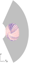 |
Fig. 1. Magnetic field lines depicting the structure of the LFFS CME model. The grey plane shows the meridional HEEQ y=0-plane. The particular realization shown in the figure has a tilt angle τCME of 90° so that the axis of symmetry in this case is corresponding to the y-axis. The tilt angle is measured from the z-axis in the yz-plane. |
 |
Fig. 2. Magnetic field components of an LFFS model with tilt angle τCME of 90.0° in the meridional plane in HEEQ coordinates. Red and blue correspond to positive and negative magnetic field components, respectively. |
2.2.2. Summary of the free parameters in the LFFS model
In the previous section, we defined the internal magnetic field structure of the CME model. In doing so, a set of parameters has been introduced. In addition to the parameters relating to the magnetic field, a full specification of the model requires additional parameters to be specified. We now list and explain these parameters in more detail and discuss possible ways to determine those parameters from observational data and/or empirical relations.
The LFFS model consists in total of ten free parameters, seven of which coincide with the free parameters of the well-known Cone model. A summary describing the parameters is presented in Table 1. The time at which the CME first reaches the inner boundary of 0.1 au is defined by the time of the onset of the launch t0. The latitude θCME, the longitude ϕCME and the speed νCME are as previously defined. The radius r0 is the radius of the CME and is assumed to remain constant as the CME is launched through the 0.1 au boundary of the computational domain. We have chosen to relate the half-width of the CME to its radius at the point in time when the centre of the CME has reached 0.1 au. This can be associated to the half-width employed in the Cone model wCME(°) via the relation r0 = 0.1 au ⋅ sinwCME. A thorough discussion of the association between the radius and half-width is presented in Scolini et al. (2018). As in the Cone model implementation in EUHFORIA, the density ρCME and temperature TCME are taken to be constant inside the CME.
Input parameters of the LFFS CME model.
The seven parameters described above can all be related to the currently widely used Cone model. Hence, they can be determined using the same methodologies as employed for the Cone model, in particular by using coronagraph images to obtain the kinematic and morphological parameters by using tools such as StereoCAT, provided by the Community Coordinated Modeling Center (CCMC) at NASA Goddard, or the forward modelling tool of Thernisien et al. (2009).
The three remaining parameters are related to the internal magnetic field structure of the CME model. As mentioned before, H(= ± 1) corresponds to the handedness of the spheromak and determines the polarity of the magnetic field inside the CME. The tilt angle τCME provides the angle with which the symmetry axis is tilted. The tilt angle is measured from the z-axis in the yz-plane, so a tilt of angle 90° corresponds to the y-axis in HEEQ as axis of symmetry as shown in Fig. 1. Finally, by using Eq. (5), the total toroidal flux F is related to the magnetic field strength B0 in Eq. (4) in the following manner
![$$ \begin{aligned}&F = \phi _t = \int \int B_\phi r \mathrm{d}r \mathrm{d} \theta \nonumber \\&\qquad \quad = \frac{2 H B_0}{\alpha ^2} \cdot \bigg [ -\sin (\alpha r_0) + \int _0^{\alpha r_0} \frac{\sin t}{t}\mathrm{d}t \bigg ]\cdot \end{aligned} $$](/articles/aa/full_html/2019/07/aa34702-18/aa34702-18-eq7.gif)
While the parameters related to the kinematics and size of the CME are closely related to those used in the Cone model, it is important to note that this is not the case for the CME speed. The speed considered for the Cone model is a combination of the translational speed νradial and the expansion speed νexpansion as directly provided by fitting the Cone model to coronagraph images. Since the Cone model does not include a magnetic field, it does not include the (additional) expansion of the CME due to the internal magnetic pressure. Hence, the initial speed required for the LFFS model should be lower than the speed of the corresponding Cone model, as the speed should reflect only the translational speed. To obtain the translational speed for the LFFS model, empirical relations that link the expansion and translation speed can be employed (see Dal Lago et al. 2003; Schwenn et al. 2005 and Gopalswamy et al. 2012). In this study, we utilize the empirical relation as proposed by Gopalswamy et al. (2012) given by
where w is the half-width of the CME. From the observed total velocity, the radial and expansion speed can then be calculated as follows
![$$ \begin{aligned} \nu _{\rm radial} = \nu _{\rm 3D}\cdot \bigg [ 1 - \frac{1}{1+\frac{1}{2}(1+\cot { w})} \bigg ], \end{aligned} $$](/articles/aa/full_html/2019/07/aa34702-18/aa34702-18-eq9.gif)
where ν3D = νradial + νexpansion. Another possibility is to estimate the expansion directly from the time-series of coronagraph images that are used to estimate the CME speed by fitting the geometrical model separately for the total extent of the emission and the core of the ejecta.
We now shortly discuss currently available methods to estimate the three parameters describing the magnetic field structure of the model. Developing a comprehensive method to determine these accurately and/or to relate them to our model input parameters, remains outside the scope of this work. First of all, the handedness can in general be determined from the magnetic polarity of the sunspots and a synthesis of observational properties inferred from the source active region as explained in more detail by Bothmer & Schwenn (1998) and Palmerio et al. (2017). The tilt angle τCME can be determined from coronagraph images when fitting a flux rope like structure that allows for a tilt, such as the graduated cylindrical shell (GCS) model Thernisien et al. (2009). However, due to the spherical symmetry of the LFFS model, the tilt is not directly equivalent to the tilt of a toroidal or cylindrical model. While these two parameters can to a degree be obtained from the available observations, the total toroidal flux of the CME is, however, poorly constrained and remains a topic of active research. Main reasons for this are that observations used to determine this parameter are based on certain assumptions, for example, that the reconnected flux is equal to the total poloidal magnetic flux of the erupted flux rope (Qiu et al. 2007). One newly proposed method to determine the toroidal flux is the so-called FRED technique (Gopalswamy et al. 2018). This method combines the line-of-sight photospheric magnetogram and post eruption arcade observations with CME coronagraph images to obtain an estimate of the toroidal flux. Evaluating the utility of such methods remains a topic of future studies.
3. Initial validation run: the events of June 17-29, 2015
3.1. Overview of the events
In Pomoell & Poedts (2018), an initial validation run of EUHFORIA that featured five CMEs using the Cone model was presented. In the this work, we will consider the same set of events in order to elucidate the effect of employing the new LFFS CME model.
During the period of 17–29 June 2015, the Sun was active with a sequence of solar eruptions occurring. The main active region responsible for most of the eruptions, NOAA AR 12371, produced three M-class flares and numerous C-class flares. A number of CMEs were also observed. The CACTUS catalogue for automated detection of transients in SOHO/LASCO coronagraph imaging observation (Robbrecht et al. 2009) lists a total of 51 events in this time period, with a total of five CMEs appearing to be clearly directed towards Earth. In the vicinity of Earth, the events were observed by the Wind spacecraft (Ogilvie et al. 1995). For the considered time window, six interplanetary shocks were detected as catalogued in the Heliospheric Shock Database2 described in Kilpua et al. (2015). With the Cone model run, Pomoell & Poedts (2018) found a clear association with the five CMEs launched and five of the detected shocks. Based on the timing of the events, the first two CMEs had a relatively low impact (quantified in terms of Dst) at Earth. The third CME, observed in coronagraph images for the first time at 02:48 UT on June 21, 2015 produced an interplanetary shock that was observed at Earth at 18:08 UT on June 22, 2015. The fourth and fifth CMEs drove interplanetary shocks that were observed at 13:07 UT on June 24, and 05:02 UT on June 25, respectively. Following the arrival of CME3, a geomagnetic storm that reached a peak DST value of −204nT on 05 UT, June 13 2015 was detected and catalogued by the provisional Dst index data maintained by the World Data Center of Geomagnetism in Kyoto, Japan. For the current study, we will focus on modelling the third CME using the LFFS model in the EUHFORIA simulations. This CME contributed to the strongest interplanetary shock and the strongest southward Bz magnetic field and was most likely largely responsible for driving the intense geomagnetic storm.
3.2. Model inputs
The empirical coronal model provides the ambient background solar wind and similarly to Pomoell & Poedts (2018), we use a GONG magnetogram that was obtained at 01:04 UT on June 25 as input to the model. This particular time was selected in Pomoell & Poedts (2018) in order to emulate an operational run in which modelling the CME (denoted CME5, see Table 2) observed on 08:36 UT on June 25 was targeted. In the present study, in contrast, we focus on modelling the CME whose shock impacted Earth at 18:08 UT June 22 as the peak in negative in-situ Bz amplitude as well as Dst index during the time period was observed as a result of this CME. Nevertheless, we employ the same magnetogram so as to retain the same ambient solar wind solution as in Pomoell & Poedts (2018).
Summary of the CME model parameters used in the modelling the 18–27 June 2015 events.
To study the effect of employing the new LFFS CME model in detail, we perform three distinct simulation runs. The first run contains Cone model CMEs for all of the five observed CMEs (hereafter called RUN1). The second run (RUN2) features a single CME using the LFFS model representing CME3 during which the largest negative Bz amplitude was observed. By including only one CME, we can elucidate the effect of neglecting previous CMEs on the plasma parameters at Earth. Finally, in the third run we employ four Cone model CMEs (CME1, 2, 4 and 5) and one LFFS CME representing CME3 (further called RUN3). This final run is important for the arrival time of the CMEs and their solution near Earth as preceding CMEs influence the environment in which later CMEs propagate, as has also been explored in Tóth et al. (2007) and Temmer et al. (2017).
We employ the same parameters as in Pomoell & Poedts (2018), where the speed of the first two CMEs has been raised slightly as to match the observed shocks and to minimize interaction with CME3. We note that as the DONKI database entries only list the kinematic parameters of the Cone model fittings, we assume each CME to have the same density ρCME = 10−18 kg m−3 and temperature TCME = 0.8 MK for both the Cone and the LFFS model. The CME model parameters used in the simulation are given in Table 2.
As discussed in detail in Sect. 2.2, when employing the LFFS model, it is important to remark that since the model includes a magnetic pressure that causes the structure to expand, the model requires as input the propagation speed as opposed to the total (expansion plus propagation) speed employed in the Cone model. For the purpose of this paper, we use the empirical relation as given by Gopalswamy et al. (2012) and Eq. (9). The empirical relation gives an expansion speed of 816 km s−1 for a CME with a half-width of 47°, and so the propagation speed that is obtained from subtracting the speed provided in the DONKI database (1250 km s−1) is 590 km s−1, which we round to 600 km s−1. For the magnetic parameters, we select the handedness to be +1 together with a 90.0° tilt angle so that we achieve a negative Bz magnetic field when the CME is arriving at Earth. Lastly, the total toroidal flux is taken to be 1014 Wb, which is the value that seems to yield the best results with the LFFS model simulations we performed so far. The input parameters for CME3 are also provided in Table 2.
3.3. Heliospheric dynamics
Figures 3–5 present snapshots from the MHD simulations for the three runs. Animated versions of the images depicting the dynamics are available in the electronic journal. In each of the figures, the top three panels represent the model run with 5 Cone model CMEs (RUN1), the middle panels represent the model run with one LFFS CME (RUN2) and finally, the bottom panels represent the model run with Cone CMEs where CME3 has been replaced with a LFFS CME (RUN3). Each subfigure shows the quantity (radial speed [km s−1], scaled number density [n(r/1 au)2, cm−3] or the co-latitude component Bθ [nT] of the magnetic field) in the heliographic equatorial plane on the left, while on the right the meridional plane that includes Earth is shown. The positions of the inner planets as well as locations for the STEREO A and B spacecraft are indicated as shown in the legend. We refrain from discussing the propagation of CMEs 1, 2, 4 and 5 as these are represented by Cone model CMEs in all the runs and have been discussed by Pomoell & Poedts (2018). Instead, we focus on detailing the propagation of the LFFS CME, corresponding to CME3 as presented in Table 2.
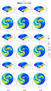 |
Fig. 3. Snapshots from the simulation showing the radial speed νr [km s−1] on June 22, 2015 at 10:03 UT, 19:03 UT and June 23, 2015 at 04:03 UT. Left panels: solution in the heliographic equatorial plane, right panels: meridional plane that includes Earth. Top row: simulation run with five Cone model CMEs. Middle row: simulation run with one LFFS CME. Bottom row: simulation run with four Cone model CMEs and one LFFS CME. In the three middle panels, the black arrows indicate where the background solar wind is restored much farther out into the domain for the Cone model run, while for the LFFS runs this is not the case. |
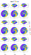 |
Fig. 4. Snapshots from the simulation showing the scaled number density n(r/1 au)2 [cm−3] on June 22, 2015 at 10:03 UT, 19:03 UT and June 23, 2015 at 04:03 UT. Left panels: solution in the heliographic equatorial plane, right panels: meridional plane that includes Earth. Top row: simulation run with 5 Cone model CMEs. Middle row: simulation run with one LFFS CME. Bottom row: simulation run with four Cone model CMEs and one LFFS CME. |
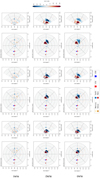 |
Fig. 5. Snapshots from the simulation for the co-latitudinal component of the magnetic field Bθ [nT] on June 22, 2015 at 10:03 UT, 19:03 UT and June 23, 2015 at 04:03 UT. Left panels: solution in the heliographic equatorial plane, right panels: meridional plane that includes Earth. Top row: simulation run with 5 Cone model CMEs. Middle row: simulation run with one LFFS CME. Bottom row: simulation run with four Cone model CMEs and one LFFS CME. |
First, we focus on the comparison between RUN1 and RUN2. In Fig. 7, isocontours of the magnetic Bz component (HEEQ coordinates) of the LFFS CME as it propagates in the inner heliosphere are shown at three different times. The top panel corresponds to a view from Earth towards the Sun, while the bottom panel provides a side view of the structure of the magnetized CME. In Fig. 3, we see that the LFFS CME (CME3) is propagating vastly slower in the simulation than the corresponding Cone CME. This will also be reflected in the timelines at Earth, as presented in Sect. 3.4. Studying Bθ, we see that for the Cone model run, some pile up of the magnetic field can be seen mainly as a result of the formation and compression at the CME shock fronts. However, for the LFFS CME, we see a clear magnetic structure propagating: a positive Bθ followed by a negative region, corresponding to a negative Bz then positive Bz in GSE coordinates (see Sect. 3.4). The propagation of a single LFFS with no additional CMEs results in a clear propagation of the front of the CME in the ecliptic.
Second, we discuss the propagation of CME3 in RUN3 where we also simulated the other four CMEs as Cone models. We notice that the CME is propagating at a similar speed as for the Cone model run. This is a combination of two factors: First, the Cone model CMEs sweep out the slow and dense background solar wind in front of CME3 so that it is able to propagate faster, and second, our LFFS model, where we lowered the initial radial speed and added a magnetic field that produces a magnetic expansion, approximately creates a similar total propagation speed for CME3. The Bθ component is noticeably interacting with the previous CME2, as CME3 was launched with a considerably higher speed than CME2.
When comparing RUN1 and RUN3, we notice that the shock fronts in both simulations look very similar for the radial speed and the density, indicating that the shocks driven by the Cone and the LFFS model have similar characteristics in the simulation regardless of the details of the driver. However, the trailing part of the CME is significantly different. Looking at the background solar wind that is inserted after CME3 has passed through the boundary, we see that the interaction is different. While for the Cone model, we observe that the background solar wind has already been restored much farther into the simulation domain, this is not the case for the LFFS model runs (see arrows in Fig. 3). This is because the LFFS CME extends much more into the heliosphere due to the magnetic expansion that acts by expanding the CME not only forward, but in all directions (see Fig. 5), and so the LFFS CME covers a larger volume in the inner heliosphere than the Cone model. The LFFS CME has a much wider spatial extent in the heliosphere and it can be seen in Fig. 6, that the shock from CME4 is pushing the magnetic field of CME3 forward in the process creating a pile up of strong magnetic field in front of the shock.
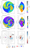 |
Fig. 6. Snapshots of the MHD simulation with four Cone CMEs and CME3 modelled as a LFFS CME for the radial speed (top panel), the scaled number density (middle panel) and the magnetic Bθ component (bottom panel) in HEEQ coordinates on June 24, 2015 at 01:04 UT. Left panels: solution in the heliographic equatorial plane, right panels: meridional plane that includes Earth. |
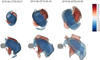 |
Fig. 7. Snapshots of the magnetic Bz structure [nT] of the LFFS CME as tracked through the inner heliosphere for different time stamps. Top panels: view from Earth towards the Sun, that is hidden behind the magnetic structure, bottom panels: side view. |
3.4. Comparison with in situ observations
Figure 8 shows plasma parameters at Earth as a function of time (blue curve) extracted from RUN2 sampled with a cadence of 10 min. Plotted from top to bottom is the radial speed, the number density, the magnetic field magnitude as well as the Bx, By and Bz components in the GSE coordinate system. In addition, five-minute averaged OMNI data is shown (thin grey curves). Interplanetary shocks as detected and catalogued in the ipshocks database Kilpua et al. (2015) for the plotted time window are shown as vertical grey dotted lines.
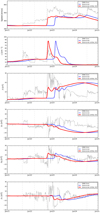 |
Fig. 8. Timelines at Earth for RUN2 (one LFFS, no Cone model CMEs) and the same timelines shifted by −8 h. We plot the radial speed, the number density, the magnitude of the magnetic field and all three magnetic field components in GSE coordinates as well as the corresponding OMNI 5 min data. |
Examining Fig. 8, it is clear that the LFFS CME is arriving late as compared to the observations, by approximately eight hours. In order to more readily compare the observations and model results, especially regarding the magnetic field components, we additionally plot the same simulation data that has been shifted in time by −8 h as a red curve in the same figure. The reason for the late arrival of the CME is addressed later in this section.
In the simulation, the transition from the ambient solar wind plasma is marked by an abrupt increase in velocity, density and magnetic field magnitude indicating a shock. Immediately after the shock, a highly disturbed region where especially the magnetic field exhibits strong oscillations is present in the observations. In this region, the Bz component briefly becomes negative before turning positive. In the simulation data, a clear shock is visible also in the magnetic field. However, the magnitude of the post-shock turbulent magnetic field is clearly lower than in the observations. Overall, this region is significantly smoothed out in the simulations most likely due to an insufficient spatial resolution to capture such turbulent structures and the lack of a turbulent sheath in the CME model. These factors also contribute to the magnitude of the magnetic field being significantly lower in this region.
At approximately 02 UT on June 23, the level of fluctuations in the observed magnetic field magnitude drops and a more consistent phase of magnetic field rotation ensues. This corresponds to the magnetic cloud of the CME, and is marked by a significant drop in the simulated Bz component. A similar, but larger drop in the OMNI 5 min data is coincident with the drop in the simulation. The overall trend from 18 UT on June 22 to 13 UT June 24 of the magnetic Bz and By components is reproduced rather well by the LFFS model. For the parameters used in this work, the model predicts an opposite sign for the magnetic Bx component. However, it is important to note that the magnetic Bz component is the largest contributor in determining the strength of the corresponding geomagnetic storm. Finally, comparing the total structure of the LFFS CME at Earth, we notice that the modelled CME is larger than observed, resulting in a slower decline of the magnitude of the magnetic field than observed. This also contributes to a larger pile-up of the magnetic field in front of later CMEs, as shown in Fig. 6.
EUHFORIA has the capability to add virtual spacecrafts at arbitrary locations in space, and we have done so for the run (RUN2) discussed above. Since we now are simulating magnetised CMEs, it is important to note that the strength and behaviour of the magnetic field observed at Earth is strongly dependent on the relative position of Earth within the magnetic cloud as it passes by. This is especially important when considering the fact that the kinematic input parameters for the CME obtained from coronagraph observations have their own errors. For instance, the propagation direction of a CME quantified by the latitude and longitude typically are accurate to approximately 10° (see e.g. ensemble modelling in Mays et al. 2015). Launching a magnetised CME with a different latitude and/or longitude may alter significantly what part of the magnetic cloud is passing by Earth. To study this, we employ virtual spacecrafts located in the vicinity of Earth. The virtual spacecraft allows us to approximate the effect of changing the direction of the CME used as input without performing a new computation.
In Fig. 10, we plot plasma parameters as a function of time for a virtual spacecraft that is located −5° latitude and −5° longitude from the position of Earth throughout the simulation for RUN2. Again, it is evident that the shock is arriving late. However, this time the lag is only approximately 4 h. Studying the magnitude of the magnetic field and the amplitude of the Bz component at this specific virtual spacecraft location, it appears that the spacecraft is located closer to the centre of the magnetic cloud. In Fig. 9, we illustrate this by plotting the magnetic field strength and the Bz component in HEEQ coordinates for a spherical slice at a constant heliocentric radius of 1 au. The x-axis corresponds to longitude (−180° − 180°) and the y-axis to latitude (−60° − 60°). The blue dot corresponds to the location of Earth. The virtual spacecraft at −5° latitude and −5° longitude is located at the white cross. This corresponds to moving towards the centre of the magnetic cloud, as expected. We are able to well reproduce the peak strength of the magnetic field magnitude and Bz component when we consider the virtual spacecraft. Nevertheless, the total duration of the magnetic cloud is still too long.
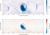 |
Fig. 9. Magnetic field strength and magnetic Bz component in HEEQ coordinates for a spherical slice at 1 au at time 2015-06-23T19-03. The blue dot corresponds to the location of Earth. The virtual spacecraft located at −5° latitude and −5° longitude from Earth is marked by the white cross. |
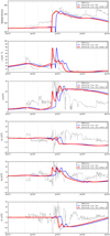 |
Fig. 10. Timelines at the location of the virtual spacecraft (−5° lat and −5° lon) for RUN2 (one LFF spheromak, no Cone model CMES) and the same timelines shifted by −4 h. We have plotted the radial speed, the number density, the magnitude of the magnetic field and all three magnetic field components in GSE coordinates as well as the corresponding OMNI 5min data. |
Why does CME3 arrive too late in RUN2? To address this issue, we now turn to discuss the other two simulation runs. In Fig. 11, plasma parameters as a function of time at Earth for the run employing four Cone CMEs and one LFFS CME (RUN3) is shown. The plot shows in addition the results of RUN1 that solely employed Cone model CMEs. From the top panel, showing the speed as a function of time, it is clear that in both RUN1 and RUN3, CME3 arrives in close agreement with the time of arrival of the shock in the observations. Therefore, we can conclude that the CME in RUN2 arrives late due to the different plasma environment that it is propagating through created by the preceding CMEs 1 and 2 as compared to the ambient solar wind. In other words, by neglecting CMEs 1 and 2, the background solar wind that CME3 is propagating through is not modelled well. As can be seen from the timeline of the radial speed and the number density at Earth, the LFFS CME propagates through a solar wind that decreases in speed as well as becomes denser. Therefore, we can expect the CME speed to be lower than observed and slowed down due to the increased drag experienced by the CME in the denser wind. As a result, the LFFS CME arrives about 8 h late. However, it is important to note that a late arrival of 8 h is within the current forecasting prediction errors (Mean Absolute Error), as discussed and presented in Riley et al. (2018), where the results of the CME arrival scoreboard are discussed.
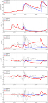 |
Fig. 11. Timelines at Earth for RUN3 (one LFF spheromak, four Cone model CMES) as well as the corresponding model run with all Cone model CMEs. We have plotted the radial speed, the number density, the magnitude of the magnetic field and all three magnetic field components in GSE coordinates as well as the corresponding OMNI 5 min data. |
In Fig. 11, timelines at Earth for the model run employing four Cone CMEs and one LFFS CME are presented. As discussed in Sect. 3.2, the insertion speeds of CME1 and CME2 have been raised compared to that of Pomoell & Poedts (2018) in order to let the shocks arrive as observed. As a result, CME3 is interacting less with CME2. However, some interaction can still be seen (see the bottom panels of Figs. 3–5). It is noteworthy that, as already discussed in Sect. 3.3, CME3 arrives at the same time both when modelled using the Cone model (RUN1) and when modelled using the LFFS model (RUN3) despite the insertion speeds being different by 850 km s−1 (see Table 1). This indicates that the reduction in speed given by the empirical model for the LFFS CME with the chosen magnetic field input values were in this case compatible and giving rise to a similar arrival time and propagation of the CME in the heliosphere.
Examining the speed as a function of time, it can be seen that for the Cone model (RUN1), the peak of the speed of CME3 is too high and declines too rapidly as compared with the observations. The same was noted also in Pomoell & Poedts (2018). For RUN3 that employs the LFFS model, the overestimation is still present, but the decline is more gradual and in better correspondence with the observations. Comparing the results of this simulation run with the run using a single LFFS CME (RUN2), we notice that both the magnitude of the magnetic field as well as the amplitude of the Bz component are lower in RUN3. This is due to the larger expansion in RUN3 as the LFFS CME propagates in more evacuated conditions, as already discussed earlier. Finally, we mention that a significant pile-up of the magnetic field of the trailing part of CME3 can be seen around June 24, 2015, when the shock of CME4 is arriving at Earth.
4. Discussion and summary
In this paper, we have detailed the implementation of a magnetised CME model into the heliospheric MHD model EUHFORIA, modelled as a linear force-free spheromak. We described the implementation of this LFFS model in detail in Sect. 2, where we focused on explaining all the input parameters of the model as well as possible ways to determine those from currently available observations and methods. In Sect. 3, we presented results of the initial validation runs that we have performed for this magnetised CME model focusing on the events occurring from June 17–29, 2015. Using a spheromak model as a magnetic CME model has multiple advantages, such as the absence of legs that remain attached to the Sun facilitating the modelling of multiple CMEs (Cone/LFFS combinations possible). Since the LFFS model is analytic, it also assures that the computation time is comparable to the Cone model runs. Hence, the method outlined in this work is computationally significantly less demanding as compared to approaches where a coronal domain is included.
The kinematic parameters of the LFFS model can all be determined from coronagraph observations similar to that of the Cone model, except for the initial speed. As discussed, the incorporation of an intrinsic magnetic field in the CME requires to disentangle the expansion from the propagation. If not accounted for, the input CME speed obtained directly is too high as it includes both the translation speed and the expansion of the CME. For the purpose of the validation run, we have opted to use the empirical relation given by Gopalswamy et al. (2012), in which the expansion speed is subtracted from the observed speed. For the magnetic field input parameters, we have opted for standard input parameters, corresponding to a flux rope-like structure arriving at Earth that corresponds to first a negative magnetic Bz component followed by a positive magnetic Bz component. A standard value of 1014 Wb for the total toroidal flux seems to correspond to a similar total expansion of the CME compared to the Cone model, as both arrive at Earth at similar times.
For the initial validation runs on the June 17–29 events, we have compared two sets of runs: we focused on one run where we modelled only the CME that produced the largest geomagnetic storm, by using the LFFS model (RUN2) and on a second run where we modelled all CMEs of the June 17–29 events by using the Cone model, except for one CME that was modelled separately using the LFFS model (RUN3). RUN1 corresponds to a run with five Cone model CMEs. For RUN2, we found that the CME arrives too late, and after comparison with the other performed simulations, this can be explained due to the difference in the plasma environment that it is propagating through as the background wind is not modified by the previous CMEs. However, the magnetised CME model was able to reproduce the magnetic field components reasonably well. Especially looking at different spacecraft locations, we found that the magnetic cloud structure that is arriving at 1 au is sensitive to a change of only a few degrees. A similar conclusion has recently been highlighted by Török et al. (2018). Keeping in mind that the error in kinematic CME parameters obtained from observations, such as latitude and longitude, can have errors larger than the discussed shift from Earth to the virtual spacecraft, it is needed to proceed with care when performing only one run with the LFFS model. One option could be to consider a grid of virtual spacecrafts close to Earth to determine a variation of the magnetic field components over those observers. However, one should proceed with care as this is not eliminating the need for ensemble modelling. With ensemble modelling the CME would be launched at a different latitude and longitude and hence it would be propagating in a different background solar wind. With virtual spacecrafts, one eliminates the computation time needed for ensemble runs, however, thus neglecting the change in interaction with the ambient wind that launching the CME in a different direction causes. More tests and parameter studies should be performed, to see if this influence is significant or not. For the run with four Cone models and CME3 modelled as a LFFS CME (RUN3), CME3 and CME2 are interacting and creating a less strong magnetic field signal compared to the single CME run with the LFFS model. For both model runs, we find that the total extent of the LFFS model in the heliosphere is larger than the observed structure. Further studies are required in order to pinpoint the source of this discrepancy.
Several efforts to improve the LFFS model, the first magnetised CME model implemented into EUHFORIA, are planned. As noted above, methods to reduce the spatial extent of the LFFS model is one topic for future studies. Another avenue is to consider employing different density structures within the LFFS CME model. Apart from improving the model, it is very important to quantify the sensitivity of each input parameter on the results. For this purpose, we are currently performing a parameter study. This is in line with the remarks made regarding the position of the magnetic cloud. At the same time, the influence of the background solar wind on the propagation of the LFFS CMEs should be studied. Finally, more reliable observational methods should be determined so that input parameters for any magnetised CME model including the LFFS model be made more reliable. The initial results presented in this work do suggest, however, that the modelling approach considered has the potential to improve the accuracy of physics-based space weather modelling.
Acknowledgments
EUHFORIA is developed as a joint effort between the University of Helsinki and KU Leuven. The validation of solar wind and CME modelling with EUHFORIA is being performed within the BRAIN-be project CCSOM (Constraining CMEs and Shocks by Observations and Modelling throughout the inner heliosphere; http://www.sidc.be/ccsom/). JP acknowledges funding from the University of Helsinki three-year grant project 490162 and the SolMAG project (4100103) funded by the European Research Council (ERC) in the framework of the Horizon 2020 Research and Innovation Programme. CV is funded by the Research Foundation – Flanders, FWO SB PhD fellowship 11ZZ216N. The computational resources and services used in this work were provided by the VSC (Flemish Supercomputer Center), funded by the Research Foundation – Flanders (FWO) and the Flemish Government – department EWI. These results were obtained in the framework of the projects GOA/2015-014 (KU Leuven), G.0A23.16N (FWO-Vlaanderen) and C 90347 (ESA Prodex).
References
- Altschuler, M. D., & Newkirk, G. 1969, Sol. Phys., 9, 131 [Google Scholar]
- Bothmer, V., & Schwenn, R. 1998, Ann. Geophys., 16, 1 [Google Scholar]
- Chandrasekhar, S. 1956, Proc. Natl. Acad. Sci., 42, 1 [NASA ADS] [CrossRef] [Google Scholar]
- Dal Lago, A., Schwenn, R., & Gonzalez, W. D. 2003, Adv. Space Res., 32, 2637 [NASA ADS] [CrossRef] [Google Scholar]
- Dumbović, M., Čalogović, J., Vršnak, B., et al. 2018, ApJ, 854, 180 [Google Scholar]
- Gibson, S. E., & Low, B. C. 1998, ApJ, 493, 460 [NASA ADS] [CrossRef] [Google Scholar]
- Gonzalez, W. D., Joselyn, J. A., Kamide, Y., et al. 1994, J. Geophys. Res., 99, 5771 [Google Scholar]
- Gopalswamy, N., Makela, P., Yashiro, S., & Davila, J. M. 2012, Sun Geosphere, 7, 7 [NASA ADS] [Google Scholar]
- Gopalswamy, N., Akiyama, S., Yashiro, S., & Xie, H. 2018, in Space Weather of the Heliosphere: Processes and Forecasts, eds. C. Foullon, & O. E. Malandraki, 335, 258 [NASA ADS] [Google Scholar]
- Gosling, J. T. 1993, J. Geophys. Res., 98, 18937 [NASA ADS] [CrossRef] [Google Scholar]
- Harvey, J. W., Hill, F., Hubbard, R. P., et al. 1996, Science, 272, 1284 [NASA ADS] [CrossRef] [PubMed] [Google Scholar]
- Hudson, H. S., Bougeret, J. L., & Burkepile, J. 2006, Space Sci. Rev., 123, 13 [NASA ADS] [CrossRef] [Google Scholar]
- Huttunen, K. E. J., Schwenn, R., Bothmer, V., & Koskinen, H. E. J. 2005, Ann. Geophys., 23, 625 [NASA ADS] [CrossRef] [Google Scholar]
- Jin, M., Manchester, W. B., van der Holst, B., et al. 2017, ApJ, 834, 173 [CrossRef] [Google Scholar]
- Kataoka, R., Ebisuzaki, T., Kusano, K., et al. 2009, J. Geophys. Res. (Space Phys.), 114, A10102 [NASA ADS] [Google Scholar]
- Kilpua, E. K. J., Lumme, E., Andreeova, K., Isavnin, A., & Koskinen, H. E. J. 2015, J. Geophys. Res. (Space Phys.), 120, 4112 [NASA ADS] [CrossRef] [Google Scholar]
- Kilpua, E., Koskinen, H. E. J., & Pulkkinen, T. I. 2017, Liv. Rev. Sol. Phys., 14, 5 [NASA ADS] [CrossRef] [Google Scholar]
- Lugaz, N., Farrugia, C. J., Winslow, R. M., et al. 2016, J. Geophys. Res., 121, 861 [Google Scholar]
- Mays, M. L., Taktakishvili, A., Pulkkinen, A., et al. 2015, Sol. Phys., 290, 1775 [CrossRef] [Google Scholar]
- Odstrčil, D., & Pizzo, V. J. 1999, J. Geophys. Res., 104, 483 [CrossRef] [Google Scholar]
- Odstrčil, D., Riley, P., & Zhao, X. P. 2004, J. Geophys. Res., 109, 2116 [Google Scholar]
- Ogilvie, K. W., Chornay, D. J., Fritzenreiter, R. J., et al. 1995, Space Sci. Rev., 71, 55 [NASA ADS] [CrossRef] [Google Scholar]
- Palmerio, E., Kilpua, E. K. J., James, A. W., et al. 2017, Sol. Phys., 292, 39 [Google Scholar]
- Pomoell, J., & Poedts, S. 2018, J. Space Weather Space Clim., 8, A35 [NASA ADS] [CrossRef] [EDP Sciences] [Google Scholar]
- Qiu, J., Hu, Q., Howard, T. A., & Yurchyshyn, V. B. 2007, ApJ, 659, 758 [NASA ADS] [CrossRef] [Google Scholar]
- Riley, P., Mays, M. L., & Andries, J. 2018, Space Weather, accepted [Google Scholar]
- Robbrecht, E., Berghmans, D., & Van der Linden, R. A. M. 2009, ApJ, 691, 1222 [NASA ADS] [CrossRef] [Google Scholar]
- Schatten, K. H., Wilcox, J. M., & Ness, N. F. 1969, Sol. Phys., 6, 442 [Google Scholar]
- Schrijver, C. J., Kauristie, K., Aylward, A. D., et al. 2015, Adv. Space Res., 55, 2745 [Google Scholar]
- Schwenn, R., dal Lago, A., Huttunen, E., & Gonzalez, W. D. 2005, Ann. Geophys., 23, 1033 [NASA ADS] [CrossRef] [Google Scholar]
- Scolini, C., Verbeke, C., Poedts, S., et al. 2018, Space Weather, 16, 754 [NASA ADS] [CrossRef] [Google Scholar]
- Shapakidze, D., Debosscher, A., Rogava, A., & Poedts, S. 2010, ApJ, 712, 565 [NASA ADS] [CrossRef] [Google Scholar]
- Shiota, D., & Kataoka, R. 2016, Space Weather, 14, 56 [NASA ADS] [CrossRef] [Google Scholar]
- Sokolov, I. V., van der Holst, B., Oran, R., et al. 2013, ApJ, 764, 23 [NASA ADS] [CrossRef] [Google Scholar]
- Temmer, M., Reiss, M. A., Nikolic, L., Hofmeister, S. J., & Veronig, A. M. 2017, ApJ, 835, 141 [Google Scholar]
- Thernisien, A., Vourlidas, A., & Howard, R. A. 2009, Sol. Phys., 256, 111 [Google Scholar]
- Török, T., Downs, C., Linker, J. A., et al. 2018, ApJ, 856, 75 [NASA ADS] [CrossRef] [Google Scholar]
- Tóth, G., de Zeeuw, D. L., Gombosi, T. I., et al. 2007, Space Weather, 5, 06003 [NASA ADS] [Google Scholar]
- van der Holst, B., Sokolov, I. V., Meng, X., et al. 2014, ApJ, 782, 81 [Google Scholar]
- Webb, D. F., & Howard, R. A. 1994, J. Geophys. Res., 99, 4201 [NASA ADS] [CrossRef] [Google Scholar]
- Xie, H., Ofman, L., & Lawrence, G. 2004, J. Geophys. Res. (Space Phys.), 109, A03109 [NASA ADS] [Google Scholar]
- Xue, X. H., Wang, C. B., & Dou, X. K. 2005, J. Geophys. Res. (Space Phys.), 110, A08103 [NASA ADS] [CrossRef] [Google Scholar]
- Yashiro, S., Gopalswamy, N., Michalek, G., et al. 2004, J. Geophys. Res., 109, A07105 [Google Scholar]
All Tables
Summary of the CME model parameters used in the modelling the 18–27 June 2015 events.
All Figures
|
Fig. 1. Magnetic field lines depicting the structure of the LFFS CME model. The grey plane shows the meridional HEEQ y=0-plane. The particular realization shown in the figure has a tilt angle τCME of 90° so that the axis of symmetry in this case is corresponding to the y-axis. The tilt angle is measured from the z-axis in the yz-plane. |
| In the text | |
|
Fig. 2. Magnetic field components of an LFFS model with tilt angle τCME of 90.0° in the meridional plane in HEEQ coordinates. Red and blue correspond to positive and negative magnetic field components, respectively. |
| In the text | |
|
Fig. 3. Snapshots from the simulation showing the radial speed νr [km s−1] on June 22, 2015 at 10:03 UT, 19:03 UT and June 23, 2015 at 04:03 UT. Left panels: solution in the heliographic equatorial plane, right panels: meridional plane that includes Earth. Top row: simulation run with five Cone model CMEs. Middle row: simulation run with one LFFS CME. Bottom row: simulation run with four Cone model CMEs and one LFFS CME. In the three middle panels, the black arrows indicate where the background solar wind is restored much farther out into the domain for the Cone model run, while for the LFFS runs this is not the case. |
| In the text | |
|
Fig. 4. Snapshots from the simulation showing the scaled number density n(r/1 au)2 [cm−3] on June 22, 2015 at 10:03 UT, 19:03 UT and June 23, 2015 at 04:03 UT. Left panels: solution in the heliographic equatorial plane, right panels: meridional plane that includes Earth. Top row: simulation run with 5 Cone model CMEs. Middle row: simulation run with one LFFS CME. Bottom row: simulation run with four Cone model CMEs and one LFFS CME. |
| In the text | |
|
Fig. 5. Snapshots from the simulation for the co-latitudinal component of the magnetic field Bθ [nT] on June 22, 2015 at 10:03 UT, 19:03 UT and June 23, 2015 at 04:03 UT. Left panels: solution in the heliographic equatorial plane, right panels: meridional plane that includes Earth. Top row: simulation run with 5 Cone model CMEs. Middle row: simulation run with one LFFS CME. Bottom row: simulation run with four Cone model CMEs and one LFFS CME. |
| In the text | |
|
Fig. 6. Snapshots of the MHD simulation with four Cone CMEs and CME3 modelled as a LFFS CME for the radial speed (top panel), the scaled number density (middle panel) and the magnetic Bθ component (bottom panel) in HEEQ coordinates on June 24, 2015 at 01:04 UT. Left panels: solution in the heliographic equatorial plane, right panels: meridional plane that includes Earth. |
| In the text | |
|
Fig. 7. Snapshots of the magnetic Bz structure [nT] of the LFFS CME as tracked through the inner heliosphere for different time stamps. Top panels: view from Earth towards the Sun, that is hidden behind the magnetic structure, bottom panels: side view. |
| In the text | |
|
Fig. 8. Timelines at Earth for RUN2 (one LFFS, no Cone model CMEs) and the same timelines shifted by −8 h. We plot the radial speed, the number density, the magnitude of the magnetic field and all three magnetic field components in GSE coordinates as well as the corresponding OMNI 5 min data. |
| In the text | |
|
Fig. 9. Magnetic field strength and magnetic Bz component in HEEQ coordinates for a spherical slice at 1 au at time 2015-06-23T19-03. The blue dot corresponds to the location of Earth. The virtual spacecraft located at −5° latitude and −5° longitude from Earth is marked by the white cross. |
| In the text | |
|
Fig. 10. Timelines at the location of the virtual spacecraft (−5° lat and −5° lon) for RUN2 (one LFF spheromak, no Cone model CMES) and the same timelines shifted by −4 h. We have plotted the radial speed, the number density, the magnitude of the magnetic field and all three magnetic field components in GSE coordinates as well as the corresponding OMNI 5min data. |
| In the text | |
|
Fig. 11. Timelines at Earth for RUN3 (one LFF spheromak, four Cone model CMES) as well as the corresponding model run with all Cone model CMEs. We have plotted the radial speed, the number density, the magnitude of the magnetic field and all three magnetic field components in GSE coordinates as well as the corresponding OMNI 5 min data. |
| In the text | |
Current usage metrics show cumulative count of Article Views (full-text article views including HTML views, PDF and ePub downloads, according to the available data) and Abstracts Views on Vision4Press platform.
Data correspond to usage on the plateform after 2015. The current usage metrics is available 48-96 hours after online publication and is updated daily on week days.
Initial download of the metrics may take a while.