| Issue |
A&A
Volume 626, June 2019
|
|
|---|---|---|
| Article Number | A131 | |
| Number of page(s) | 12 | |
| Section | Interstellar and circumstellar matter | |
| DOI | https://doi.org/10.1051/0004-6361/201935482 | |
| Published online | 24 June 2019 | |
Opening the Treasure Chest in Carina★
1
Tata Institute of Fundamental Research,
Homi Bhabha Road,
Mumbai
400005,
India
e-mail: This email address is being protected from spambots. You need JavaScript enabled to view it.
2
Institute for Astronomy, University of Hawaii,
640 N. Aohoku Place,
Hilo,
HI
96720,
USA
3
Max Planck Institut für Radioastronomie,
Auf dem Hügel 69,
53121
Bonn,
Germany
4
USRA/SOFIA, NASA Ames Research Center,
Mail Stop 232-12, Building N232, PO Box 1,
Moffett Field,
CA
94035-0001,
USA
Received:
18
March
2019
Accepted:
7
May
2019
Abstract
Pillars and globules are the best examples of the impact of the radiation and wind from massive stars on the surrounding interstellar medium. We mapped the G287.84-0.82 cometary globule (with the Treasure Chest cluster embedded in it) in the South Pillars region of Carina (i) in [C II], 63 μm [O I], and CO(11–10) using the heterodyne receiver array upGREAT on SOFIA and (ii) in J = 2–1 transitions of CO, 13CO, C18O, and J = 3–2 transitions of H2CO using the APEX telescope in Chile. We used these data to probe the morphology, kinematics, and physical conditions of the molecular gas and the photon-dominated regions (PDRs) in G287.84-0.82. The velocity-resolved observations of [C II] and [O I] suggest that the overall structure of the pillar (with red-shifted photoevaporating tails) is consistent with the effect of FUV radiation and winds from η Car and O stars in Trumpler 16. The gas in the head of the pillar is strongly influenced by the embedded cluster, whose brightest member is an O9.5 V star, CPD −59°2661. The emission of the [C II] and [O I] lines peak at a position close to the embedded star, while all the other tracers peak at another position lying to the northeast consistent with gas being compressed by the expanding PDR created by the embedded cluster. The molecular gas inside the globule was probed with the J = 2–1 transitions of CO and isotopologs as well as H2CO, and analyzed using a non-local thermodynamic equilibrium model (escape-probability approach), while we used PDR models to derive the physical conditions of the PDR. We identify at least two PDR gas components; the diffuse part (~ 104 cm−3) is traced by [C II], while the dense (n ~ 2–8 × 105 cm−3) part is traced by [C II], [O I], and CO(11–10). Using the F = 2–1 transition of [13C II] detected at 50 positions in the region, we derived optical depths (0.9–5), excitation temperatures (80–255 K) of [C II], and N(C+) of 0.3–1 × 1019 cm−2. The total mass of the globule is ~1000 M⊙, about half of which is traced by [C II]. The dense PDR gas has a thermal pressure of 107–108 K cm−3, which is similar to the values observed in other regions.
Key words: ISM: molecules / ISM: lines and bands / photon-dominated region / submillimeter: ISM / ISM: clouds
A copy of the reduced datacubes (FITS files) is available at the CDS via anonymous ftp to cdsarc.u-strasbg.fr (130.79.128.5) or via http://cdsarc.u-strasbg.fr/viz-bin/qcat?J/A+A/626/A131
© ESO 2019
1 Introduction
Some of the most spectacular structures in the molecular interstellar medium (ISM) are observed in the vicinity of hot O/B stars or associations in the forms of cometary globules and pillars. The cometary globules arise when the expanding H II region due to the O/B star overruns and compresses an isolated nearby cloud causing it to collapse gravitationally. As the cloud contracts the internal thermal pressure increases causing the cloud to re-expand, so that a cometary tail is formed that points away from the exciting star. A high-density core develops at the head of the globule, which could collapse to form one or more stars. The pillars arise when an ionization front expands into a dense region that is embedded in the surrounding molecular cloud, so that a cometary tail or pillar forms due to the shadowing behind the dense clump. The pillar so formed is supported against radial collapse by magnetic field but undergoes longitudinal erosion by stellar winds and radiation. There exist multiple analytical (Bertoldi 1989; Bertoldi & McKee 1990) and numerical models (Lefloch & Lazareff 1994; Bisbas et al. 2011), which explain and reproduce many of the observed features of these structures sculpted by the radiation and wind from massive O/B stars starting from either an isolated or an embedded, pre-existing dense clump or core. There also exist observations which find the presence of sequential star formation in such structures consistent with triggered formation of stars due to the photoionization-induced shocks (Sugitani et al. 2002; Ikeda et al. 2008). However, numerical simulations are yet to provide any strong evidence supporting the enhanced formation of stars due to triggering by the ionization fronts. Physically the scenario is complex due to the simultaneous influence of radiation, magnetic field, and turbulence on the evolution of such clouds. Since the pillars and globules are regions in which the gas is strongly influenced by radiation, observation of the emission from the photon-dominated regions (PDRs) as traced by the [C II] at 158 μm, [O I] at 63 μm, and mid- and high-J CO lines are ideal to constrain the physical conditions of these regions.
The Carina nebula cluster (NGC 3372) is the nearest (d = 2.3 kpc) massive star-forming region in the southern hemisphere with more than 65 O stars (Smith et al. 2010). Early surveys in molecular lines and far-infrared continuum of the central parts of the Carina nebula suggested that the radiation and stellar winds from hot massive stars in the region are clearing off the remains of their natal cloud (Harvey et al. 1979; de Graauw et al. 1981; Ghosh et al. 1988). The southeastern part of the nebula is particularly rich in large, elongated, bright pillars, all of which seem to point towards η Carina and Trumpler 16, a massive open cluster with four O3-type stars, as well as numerous late O and B stars. Studies of this region, called the South Pillars, in the thermal infrared and radio suggest that it is a site of ongoing and possibly triggered star formation (Smith et al. 2000, 2005; Rathborne et al. 2004). Since the pillars in this region have the bright parts of their heads pointing towards η Car and their extended tails pointing away from it, it seems clear that they are sculpted by the radiation and winds from the massive stars associated with Trumpler 16 and η Car.
One of the cometary globules in the South Pillars, G287.84-0.82, is known to have a dense compact cluster embedded in the head of the globule. This cluster, called the Treasure Chest (Smith et al. 2005), contains more than 69 young stars and Oliveira et al. (2018) estimate a cluster age of 1.3 Myr. The most massive cluster member is CPD −59°2661 (at αJ2000 = 10h 45m 53.s713, δJ2000 = −59°57′ 3″. 8), which is an O9.5 star (Walsh 1984; Hägele et al. 2004) that illuminates a compact H II region seen in Hα and in PDR emission (Thackeray 1950; Smith et al. 2005), see Figs. 1 and 2. To the north and east of the star, the surrounding dense molecular cloud prevents the H II region from expanding. Here the distance from the expanding H II region to the star is only ~ 12′′, while it appears to be expanding freely to the west where the gas densities are low (Fig. 2). The bright star ~ 30′′ northeast of CPD −59°2661 (saturated in IRAC images) is probably a member of the embedded cluster. This star (Hen 3-485 = Wra 15-642) is a Herbig Be star (Gagné et al. 2011). It is reddened by ~ 2 mag and has strong infrared excess. It is associated with an H2O maser with a single maser feature at the same velocity of the globule (Breen et al. 2018). The vibrationally excited H2 observations of Treasure Chest by Hartigan et al. (2015) show the external PDR illuminated by η Car. They also show an internal PDR excited by CPD −59°2661, which expands into the head of the globule. Thus, while the cometary globule around the Treasure Chest cluster appears to have been shaped by the radiation from the massive stars, the embedded, young stellar cluster illuminates its own PDR in the head of the globule and will eventually dissociate the surrounding molecular cloud. In this paper we present mapping observations of the [C II] at 158 μm, [O I] at 63 μm, and CO emission of G287.84-0.82 in Carina to derive a better understanding of the influence of η Carina, O stars in Trumpler 16 and the embedded Treasure Chest cluster on the physical conditions of the globule.
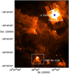 |
Fig. 1 Spitzer IRAC 8 μm image of South Pillars of Carina showing the location of the Treasure Chest region on a larger perspective. The image artifacts from the exceedingly bright O2 star η Carina, marked by a star symbol, completely hides the massive OB cluster, Trumpler 16, located just southwest of it. The G287.84 pillar is shown with a rectangle. |
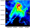 |
Fig. 2 Spitzer 8 μm image of the cometary globule G287.84-0.82. One can see three tails extending to the south from the head part of the globule. All tails point away from η Car and the O stars in Trumpler 16, which are to the northwest of the globule, see Fig. 1. The internal PDR, illuminated by CPD −59°2661 in the Treasure Chest cluster, is seen as a bright semi-shell in the northern part of the image. A secondary pillar, which we call the “duck head”, is west of the Treasure Chest cluster. It also has an embedded young star in the head. Faint foreground PDR emission is seen all around the globule, especially to the north. We have marked the position of CPD −59°2661 and Hen 3-485. The two dashed lines indicate the cuts for position–velocity plots discussed later in the text. The extraction positions of spectra discussed in Sect. 3 are labeled 1–8. |
2 Observations
2.1 SOFIA
We have retrieved [C II] and CO(11–10) observations of G287.84-0.82 (the Treasure Chest) from the data archive of the Stratospheric Observatory for Infrared Astronomy (SOFIA; Young et al. 2012). The observations (PI: X. Koenig) were part of a larger program (01_0064) on observing irradiated pillars in three massive star forming regions. The observations were done with the German REceiver for Astronomy at Terahertz frequencies (GREAT1 ; Heyminck et al. 2012) in the L1/L2 configuration on July 22, 2013 during the New Zealand deployment. These observations were made on a 70-min leg at an altitude of 11.9 km. The L1 mixer was tuned to CO(11–10), while the L2 mixer was tuned to the [C II] 2P3∕2 → 2P1∕2 transition, see Table 1 for observation details. The backends were fast Fourier transform spectrometers (AFFTS; Klein et al. 2012) with 8192 spectral channels covering a bandwidth of 1.5 GHz, providing a frequency resolution of 183.1 kHz. The Treasure Chest was mapped in total power on-the-fly mode with a one-second integration time and sampled every 8′′ for a map size of 248′′ × 168′′. The map was centered on (α, δ) = (10h 45m55.s05, −59°57′41.′′2) (J2000) with an off-position 5′ to the south. All offsets mentioned in the text and figure captions hereafter refer to this center position. Here we have only used the CO(11–10) data because the [C II] observations made with upGREAT (see below) are of superior quality.
The source G287.84-0.82 was also observed with upGREAT in consortium time from Christchurch on June 14, 2018 on a 65-min leg at an altitude of 11.4–12.4 km. The upGREAT was in the Low Frequency Array/High Frequency Array (LFA/HFA) configuration with both arrays operating in parallel. The 14-beam LFA array (Risacher et al. 2016) was tuned to [C II], while the 7-beam HFA array was tuned to the 3 P1–3P2 63 μm [O I] line. The spectrometer backends are the last generation of fast Fourier transform spectrometers (FTTS; Klein et al. 2012). They cover an instantaneous intermediate frequency (IF) bandwidth of 4 GHz per pixel, with a spectral resolution of 142 kHz. To ensure good baseline stability for the [O I] line, we mapped the Treasure Chest in single seam switch (SBS), on-the-fly mode by chopping to the east of the cometary globule. The region we chopped to appear free of [C II] emission, even though there is widespread, faint foreground emission at velocities of approximately −30 to −24 km s−1 in the area around the globule. We split the region into two submaps. The northern part of the globule was done as a 123′′ × 69′′ map with a chop amplitude of 120′′ at a position angle (PA) of 60°. The map was centered with an offset of 0′′,+27′′ relative to our track position and sampled every 3′′ with an integration time of 0.4 s. The second map had a size of 231′′ × 93′′ and was centered at an offset of −9′′,−54′′. For this map we used a chop amplitude of 135′′ at a PA of 84°. This setup provided us with a fully sampled map in [O I] over most of the globule and an over-sampled map of [C II] with excellent quality.
The atmospheric conditions were quite dry. The zenith optical depth for [C II] varied from ~0.19 at the beginning of the leg to ~0.15 at the end of the leg. The system temperatures for most pixels were about 2400 K, some around 2900 K, and three outliers had higher system temperatures of 3300–4000 K. One noisy pixel was removed in the post-processing. Beam efficiencies were applied individually to each pixel, see Table 1. For [O I] the zenith optical depth varied between 0.24 and 0.43, and system temperatures ranged from 2900 to 4650 K excluding one noisy pixel, which was not used.
All the GREAT data were reduced and calibrated by the GREAT team. This processing involved correction for atmospheric extinction (Guan et al. 2012). The calibrated data in antenna temperature scale,  were converted to main beam antenna temperature, Tmb using a forward scattering efficiency of 0.97. The final data cubes were created using CLASS2 and maps were created with a velocity resolution of 0.5 km s−1. The rms noise per map resolution element with 0.5 km s−1 velocity resolution is ~1.3 K for the CO(11–10) map, 0.70 K for [C II], and 2.4 K for [O I].
Observation details: frequencies, receivers, beam sizes, and beam efficiencies.
2.2 APEX
G287.84-0.82 was observed on March 28, 2017 using the PI230 receiver on the 12 m Atacama Pathfinder EXperiment (APEX3) telescope, located at Llano de Chajnantor in the Atacama desert of Chile (Güsten et al. 2006). PI230 is a dual sideband separating, dual polarization receiver. Each band has a bandwidth of 8 GHz, and therefore each polarization covers 16 GHz. Each band is connected to two Fast Fourier Transform fourth Generation spectrometers (FFTS4G; Klein et al. 2012) with 4 GHz bandwidth and 65 536 channels, providing a frequency resolution of 61 kHz, in other words a velocity resolution of ~ 0.079 km s−1 at 230 GHz. The PI230 receiver can be set up to simultaneously observe CO(2–1), 13CO(2–1), and C18O(2–1). This frequency setting also includes three H2CO lines and one SO line in the lower sideband (see Table 1) all of which were detected in G287.84-0.82.
G287.84-0.82 was mapped in on-the-fly, total power mode and sampled every 10′′ with an integration time of 0.5 s. The map size was ±100′′ in right ascension (RA) and from −150′′ to +95′′ in declination (Dec). The off position used in these observations was at RA =10h49m14s, Dec = −59°35′40′′ (J2000). The weather conditions were quite good for 1.3 mm observations. The zenith optical depth varied from 0.146 to 0.156 at 230 GHz resulting in a system temperature of ~ 155 K.
The final data cubes were created using CLASS by re-sampling the spectra to 0.5 km s−1 velocity resolution. The rms noise per map resolution element (half a beam width) is ~ 0.18 K.
3 Results
Figure 3 shows a comparison of the integrated intensity image (in K km−1) of [C II] at 158 μm (contours) overlaid on fluorescent H2, 8 μm PAH emission, 160 μm dust continuum, as well as on integrated intensity images of most spectral lines that we have mapped. The CO, 13CO, and 160 μm dust continuum images show that the G287.84-0.82 cloud has the shape of a cometary globule with three spatially separated extensions or tails in the south, which all point away from η Car and Trumpler 16. The η Car is to the northwest, approximately at a projected distance of 12 pc from G287.84-0.82. There is a secondary cloud surface ~60′′ south of CPD −59°2661, which is alsoroughly perpendicular to η Car. On the western side there is a narrow, second pillar with a head that looks like the head of a duck, and which we call the “duck head”, see Fig. 3 in Smith et al. (2005) and Fig. 2 here. The structure of the cloud is consistent with it being exposed to and shaped by the UV radiation and stellar winds from η Car and from the O3stars in Trumpler 16. The [C II] emission matches extremely well with the other bona fide PDR tracers like the fluorescent H2, 8 μm PAH and [O I] 63 μm emission, suggesting that most of the [C II] emission originates in the irradiated cloud surfaces. The PDR gas inside the pillar forms a shell aroundthe Treasure Chest cluster. Here the emission appears to be dominated by the stellar cluster with only a minor contribution from the externally illuminated cloud surfaces. High-density tracers like CO(11–10), C18O(2–1), H2CO(303–202) and SO (the latter only shown as a velocity-channel map in Fig. A.6) all peak to the northeast of the positions of both the PDR peak and the embedded star cluster. The distribution of intensities and the relative location of the high-density peak suggest that the head of the cloud is more compressed towards the northeastern edge, and the PDR shell curving around the Treasure Chest cluster shows that the expanding H II region both heats up and compresses the surrounding cloud, especially to the northeast. Clear detection of H2CO and CO(11–10) at the position of the column density peak suggest gas densities in excess of 105 cm−3.
Figure 4 shows the channel maps for the [C II] and [O I] 63 μm emission. Both maps show that the bulk of the gas in the head of the region is at a velocity of approximately −14.5 km s−1, while the tails are generally red-shifted. This suggests that the globule is somewhat behind η Car, which has a radial velocity of −20 km s−1 (Smith 2004), so that the stellar wind and the radiation pressure from the star push them in the radial direction from η Car, making them appear red-shifted. The higher angular resolution of the [O I] 63 μm observations (particularly around υ = −13 km s−1 in Fig. 4) helps identify the dense PDR shell around CPD −59°2661. The [C II] channel maps also show a tail-like structure to the east at a velocity of approximately −15 km s−1, which is not seen in [O I] 63 μm or CO(11–10) emission (Fig. A.1). The comparison with channel maps of all observed CO, H2CO, and SO lines (Figs. A.1–A.6), show that the “eastern tail-like” −14.8 km s−1 component is clearly detected in the CO(2–1) channel maps and only partially in the 13CO(2–1) channel maps. This suggests that the −14.8 km s−1 emission component in the tail has lower density, since it is not detected in the transitions, which either (a) have high critical density like [O I], CO(11–10), and H2CO, or (b) trace regions of high column density, for example, C18O(2–1). This gas is probably part of the halo around the globule, which has not yet been affected by the wind from η Car.
We next compared the spectra of the different tracers at eight selected positions which are marked in Fig. 2. These positions are selected to sample positions in the head of the globule (#3 to #5), as well as some specific features, such as the CO peak (#1), the [C II] peak (#2), the duck neck (#6), the duck head (#7), and the eastern tail (#8). Since the line profiles of the J=2–1 transitions of CO (and isotopologs) are similar, we only show the 13CO spectra along with other spectra in Fig. 5. At the position of the column density peak (#1), we find that all spectra have similar line widths, with [O I] being slightly broader than the others. At position #2 the PDR tracers [C II] and [O I] are significantly broader than the molecular gas tracers. Table 2 gives the result of fitting the spectra using a single Gaussian velocity component for all positions except position #8 where we fitted two Gaussian velocity components. We note that for positions #7 and #8 only the tracers that are detected are presented in Table 2.
We find that except for position #1, the [C II] and [O I] lines are broader than the CO lines by 1–1.5 km s−1. The line widths and spectral line profiles of [C II] and [O I] match very well, suggesting that both [O I] and [C II] emissions originate in PDR gas with no significant contribution from (a) shocks to [O I] and (b) the H II region to the [C II] emission. A closer inspection of the [O I] and [C II] data in the head of the globule suggests that although the outer profiles of the spectra from the two species match well, the [O I] spectra show a flattened or double-peaked profile close to the column density peak and further southeast (e.g., positions 1, 3, and 5 in Fig. 5), whereas the [C II] spectra always show a smooth, single-peaked Gaussian profile. The two velocity components detected in CO, 13CO, [C II], and [O I] at position #8, correspond to the main globule and the red-shifted eastern tail.
Figure 6 shows para-H2CO spectra at three positions where all three transitions J = (303–202), (322 –221), and (321 –220) are detected with good S/N. The strongest transition, J = (303–202), is detected over a much larger area around the column density peak (as shown in Figs. 3 and A.6). At the positions (0,26) and (15,26), the para-H2CO 303–202 transition shows a single-peaked profile, while at (0,40), where the line is the strongest, there is a hint of a red-shifted component. The position of the peaks of the two fainter transitions match with the brighter peak. The widths of the H2CO lines match well with the line widths of the other molecular lines at these positions. The emission from the (65 → 54) transition of SO spans an even narrower range of velocities and is mostly confined to the higher-density head-region of the globule (Fig. A.6).
The high S/N of the observed [C II] spectra allows us to simultaneously detect the brightest hyperfine component, F = 2–1, of the 13C+ fine structure line at 50 positions in the area we have mapped. If we average these spectra together, we also see the two fainter hyperfine transitions F = 1–0 and F = 1–1 of [13C II]. However, they are too faint in individual positions for a meaningful analysis, hence we only used the F = 2–1 transition for this purpose. Figure 7 shows examples of [13C II] F = 2–1 line, which is offset by +11.2 km s−1 from the [C II] line, at two selected positions. The line-integrated intensity of the [13C II] line was obtained by fitting the [CII] and [13C II] lines simultaneously. In this fitting procedure the brighter [C II] line is fitted first, and the fainter [13C II] line is constrained to be located at a velocity relative to the brighter component given by the velocity separation of the two transitions.
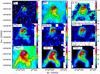 |
Fig. 3 Contours of intensity integrated between −20 and −5 km s−1 of [C II] (black contour) overlayed on false-color images of tracers mentioned in the panels. Top row: tracers of PDR gas, middle row: tracers of high-density gas, bottom row: tracers of overall gas and dust distribution in the region. The filled asterisk shows the position of CPD −59°2661. The color scale for each panel is shown next to the panel and the units are K km s−1 for the spectral lines, MJy sr−1 for 8 μm and Jy pixel−1 for PACS (3′′ pixel). The values of [C II] contours are 10–100% of the peak intensity of 505 K km s−1. |
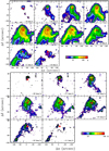 |
Fig. 4 Channel maps of [C II] (top) and [O I] 63 μm (bottom) emission. Velocities corresponding to the channel are marked in each panel. The red star marks the position of CPD −59°2661. The positional offsets are relative to the center α = 10h45m55.s05, δ = −59d57m16.′′7 (J2000). |
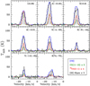 |
Fig. 5 Comparison of emission spectra of [C II] (filled histogram), 13CO(2–1) (red), CO(11–10) (green), and [O I] 63 μm (black) at selected positions shown in panel 2 of Fig. 3. The 13CO, CO(11–10), and [O I] spectra are multiplied by factors of 4, 2, and 3, respectively. |
4 Analysis
4.1 Local thermodynamic equilibrium (LTE) and non-LTE analysis of molecular emission
We derived a first-order estimate of the total column density of the gas using the observed integrated line intensities of CO and 13CO J = 2–1. Since the CO(2–1) emission is mostly optically thick, we used the maximum temperatures for CO(2–1) as the kinetic temperature (Tkin). We further assumed that Tex for all the isotopes of CO are identical and equal to Tkin. For all pixels where both CO and 13CO is detected, we estimated the N(13CO) to lie between (1.3–76) × 1015 cm−2. Using a 12CO/13CO ratio of 65 (Rathborne et al. 2004), and CO/H2 = 10−4, we found N(H2) to range between 8.5 × 10²⁰ and 4.9 × 1022 cm−2. This estimate of N(H2) agrees well with what Breen et al. (2018) found from observations of NH3 (1,1) and (2,2) with the Australia Compact Array (ATCA), 2.2 × 10²² ± 0.9 × 1022 cm−2, as well as with the estimate by Rebolledo et al. (2016), which was based on observations of J = 1–0 transitions of 12CO and 13CO. It also matches reasonably well with the column density estimated by both Roccatagliata et al. (2013) and Schneider et al. (2015) based on dust continuum observations with the Herschel Space Observatory. Our estimate of the CO column density, 8.5 × 10¹⁶–4.9 × 1018 cm−2, is also consistent with the results by Rathborne et al. (2004), who used CO(2–1) and CO(1–0) observed with Swedish ESO Submillimeter Telescope (SEST) to derive Tex = 40 K and N(CO) = 1.4 × 1018 cm−2.
The intensity ratios of the 303 –202/322–221 and the 303 –202/321–220 transitions of para-H2CO are good thermometers for determining kinetic temperature (Mangum & Wootten 1993). The 321 –220 has a slightly better S/N than 322 –221 in the three positions. Therefore, we use the observed 321 –220/303–202 ratios to estimate the kinetic temperature (Tkin) in these positions. To constrain the kinetic temperature, density, and column density of the gas, a grid of models based on the non-local thermodynamic equilibrium (non-LTE) radiative transfer program RADEX (van der Tak et al. 2007) was generated and compared with the intensity ratios of para-H2CO. Model inputs were molecular data from the LAMDA database (Schöier et al. 2005) and para-H2CO collisional rate coefficients from LAMDA (Wiesenfeld & Faure 2013). RADEX predicts line intensities of a given molecule in a chosen spectral range for a given set of parameters: kinetic temperature, column density, H2 density, background temperature, and line width. A value of 2.73 K was assumed as the background temperature for all calculations presented here. The synthetic line ratios were calculated for a line width of 2 km s−1, similar to the line widths we deduced for the three positions. The observed line ratios of 303 –202/321–220 at the three positions (14,26), (0,26), and (0,40) are 3.0, 3.4, and 4.4, respectively. We generated a grid of models with Tkin = 20–120 K, n(H2) = 104 –107 cm−3 and N(H2CO) = 1012 –1015 cm−2. Figure 8 shows a plot of the predicted 303 –202/321–220 ratios as a function of Tkin and N(H2CO) for n(H2) = 105 and 106 cm−3. The observed values of the H2CO ratios are shown as contours, which effectively constrain the temperature up to N(H2CO) of 2 × 1013 cm−2. Based on observations of high-mass, star-forming clumps, the value of N(H2CO)/N(H2) ranges between 10−10 and 10−9, which corresponds to N(H2CO) of 1012 –1013 cm−2 for the derived N(H2) of ~ 1022 cm−2 for the globule.
The critical density of the H2CO transitions that we observed is 1–6 × 10⁵ for 50 K gas (Shirley 2015) and the critical densities for low-J CO and NH3 are much lower (~ 103 cm−3 for NH3). Thus, while a density of 104 cm−3 is too low, n(H2) of 106 cm−3 appears to be too high. We therefore assumed a gas density of n(H2) = 105 cm−3, which we considered to be a reasonable compromise. The outcome of the analysis stays about the same even for slightly higher densities. With the assumption of a gas density of n(H2) = 105 cm−3, we obtain kinetic temperatures of 55, 75, and 90 K, respectively. However, we note that since the H2CO lines are weak, the uncertainties in Tkin determined from spectra at individual positions are also high. In order to derive a more reliable estimate of Tkin we averaged the H2CO lines over an area where all three lines are detected. The observed line ratios then lie in the range of 3.2–3.4 for 322 –221 and 321 –220, respectively. The average kinetic temperatures are therefore in the range of 60–70 K. Breen et al. (2018) used NH3 (1,1) and (2,2), another accurate molecular gas thermometer (Wamsley & Ungerechts 1983), to derive a rotational temperature, Trot, of 23 K averaged over the area where both (1,1) and (2,2) were detected. This corresponds to a kinetic temperature of 39 K, which is similar to what we derived from CO(2–1). The kinetic temperatures estimated from far-infrared dust emission (Roccatagliata et al. 2013), are somewhat lower. Roccatagliata et al. (2013) find ~ 32 K for the head region and ~ 25 K for the column density peak. Thus, the Tkin derived from H2CO is higher than other estimates, although the reason for this discrepancy is not clear.
Results of single (or double for position #8) component Gaussian fitting of observed spectra.
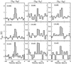 |
Fig. 6 Spectra of the J = (303–202), (322 –221), and (321–220) transitions of para-H2CO at selected positions where the fainter lines are clearly detected. |
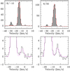 |
Fig. 7 Examples of [C II] spectra at two positions where [13C II] is also detected. The emission feature at approximately −28 km s−1 is from faint foreground PDR emission unrelated to the globule. The lower panels show an expanded view of the [13C II] lines, along with the result of simultaneous fitting of [C II] and [13C II] lines as describedin the text. |
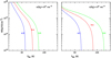 |
Fig. 8 RADEX non-LTE modeling of 303–202/321–220 ratio of H2CO. The ratio is calculated as a function of the gas kinetic temperature (Tkin) and column density of H2CO for the volume densities n(H2) of 105 (left) and 106 cm−3 (right). Contours with labels mark the observed line-intensity ratios for H2CO. |
4.2 C+ column density
While [C II] is mostly known to be optically thin, recent velocity-resolved observations of Galactic, massive star-forming regions have shown that this is not always the case, because the detection of strong hyperfine transitions of 13C+ indicate that [C II] can be significantly optically thick (Mookerjea et al. 2018; Ossenkopf et al. 2013, among others). If [13C II] is not detected, the determination of C+ column density, N(C+) requires either assumptions about the excitation temperature, or use of the same excitation temperature as molecular emission. Simultaneous detection of the [C II] and [13C II] lines is independent of calibration errors, and allow us to determine the excitation temperature and optical depth, if [C II] is optically thick. The F = 2–1 hyperfine line of [13C II] was detected in 50 positions. As described in Sect. 3, we derived the integrated line-intensities of the [13C II] emission at all these positions and below we estimate the  and N(C+) following the formulation by Ossenkopf et al. (2013).
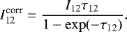
The optical depth τ12 of the [C II] line was determined using Eq (1), where I12 and I13 represent  and
and  respectively, and
  = 65 (Rathborne et al. 2004). The derived optical depth for [C II] ranges between 0.9 and 5.
![Mathematical equation: \begin{equation*} \frac{I_{\textrm{12}}}{I_{\textrm{13}}} = \frac{{}^{12}\textrm{C}}{{}^{13}\textrm{C}}\left[\frac{1-\exp(-\tau_{12})}{\tau_{12}}\right]\!.\end{equation*}](/articles/aa/full_html/2019/06/aa35482-19/aa35482-19-eq6.png) (1)
(1)
The optical depth-corrected, integrated intensity of [C II] is derived from Eq. (2).
 (2)
(2)
Subsequently, the excitation temperature of [C II] ( ) is derived using Eq. (3) which was obtained by dividing Eq. (1) by Eq. (3) from Ossenkopf et al. (2013).
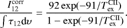 (3)
(3)
The values of  vary between 80 and 255 K. Most positions show values between 110 and 130 K, which is consistent with the Tkin derived (Sect. 4.1) from H2CO and CO(11–10).
Becausewe know the optical depth and the excitation temperature, we can now estimate the column density of C+ by inverting the following Eq. (4) (Eq. (3) of Ossenkopf et al. 2013). We obtained column density of C+ ranging 3–7 × 1018 cm−2.
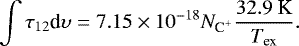 (4)
(4)
4.3 Mass of the cometary globule
Having mapped most of the globule in CO(2–1) and isotopologs, we were able to use our maps to estimate the total mass of the globule. For this we used 13CO(2–1) and computed a column density for each pixel in the map, where 13CO(2–1) is detected. We used the LTE approximation for the column density, estimating Tex from the peak of 12CO at the same position and then deriving the opacity τ for 13CO, following the method outlined in White & Sandell (1995). With the assumptions that  = 65 and
  = 10−4, we found a total mass of ~ 600 M⊙.
We derived similar mass estimates from the observed [C II] intensities by assuming the line to be optically thin, a gas density of n = ncr = 3000 cm−3, and an excitation temperature of Tex = 100 K. If we assume that half of the available carbon is in C+ (0.65 × 10⁻⁴), then the total mass of the globule seen in [C II] is ~440 M⊙, which is comparable to what we derived from 13CO(2–1). This is an underestimation, since we know that there are positions where [C II] is optically thick. The fraction of pixels where [C II] is optically thick, however, is only ~8% of all pixels in which [C II] was detected. Therefore, we underestimated the mass at most by 15%. The uncertainty in our mass estimate is completely dominated by the amount of carbon that is in the form of C+.
The masses we derived from CO and C+ closely agree with the value of 1200 M⊙ estimated from the 1.2 mm dust continuum emission by Rathborne et al. (2004). The mass estimates from different tracers are therefore comparable and suggest a total mass of the globule of ~ 1000 M⊙.
4.4 Position–velocity diagrams along the cuts
In order to understand how the PDR emission relates to the molecular gas in the globule, we made position–velocity (PV) plots in [C II], [O I], and 13CO(2–1) along the two cutsshown in Fig. 2. The PV plots were made using the task velplot in Miriad (Sault et al. 1995). Velplot uses a 3 × 3 pixel interpolation kernel resulting in beam sizes of 21″. 2, 11″. 1, and 28″. 5 for [C II], [O I], and 13CO(2–1)4, respectively.Figure 9 shows the PV plots along the cut going from (top) northwest to southeast (NW-SE), and (bottom) northeast to southwest (NE-SW).
Along the NW-SE cut, the PDR tracers rise sharply in the northwest and then fall off and become narrower after passing through the H II region powered by CPD −59°2661. The tail region is distinctly red-shifted in the eastern tail of the globule, although both [C II] and 13CO(2–1) show a velocity component at −14.5 km s−1, probably arising from unperturbed gas from the head of the globule. As we saw above from the channel maps, this velocity component is not seen in C18O or [O I], suggesting that it is more diffuse, low-density gas. The [C II] and [O I] PV plots show clear peaks where the cut intersects the PDR shell that is illuminated by CPD −59°2661, while 13CO(2–1) peaks a bit further south. The 13CO(2–1) line width remains unchanged across the PDR shell, which indicates that the molecular gas in the globule is not yet affected by the expanding H II region.
In the NE-SW position–velocity plot, the PDR shell stands out clearly in [C II] and [O I] being more blue-shifted close to the exciting star (marked by O in Fig. 9), while 13CO(2–1) peaks at the molecular column density peak. [O I] and [C II] also have peaks at the southwestern PDR rim of the main globule. [O I] is not present in the low-density region between the main globule and the duck neck; 13CO(2–1) is very faint or absent as well. [C II], however, is relatively strong and distinctly red-shifted, presumably low-density gas expanding from the PDR region illuminated by CPD −59°2661. Both [C II] and [O I] show extended emission on the side of the neck facing towards the Treasure Chest, indicating that the neck is associated with the PDR region illuminated by CPD −59°2661. At the angular resolution of our observations the northern PDR illuminated by η Car and the PDR shell illuminated by CPD −59°2661 blend together, whereas they are seen as two separate PDRs in the 8 μm image, see Fig. 2. The northern PDR, however, is close to the systemic velocity of the globule head, while the internal PDR shell is more blue-shifted north of the star. In the NE-SW cut we see a similar jump in velocity between the external PDR rim and the PDR shell.
Both PV plots show that there is [C II] emission outside the thin PDR interface of the globule. This is the same photo-evaporated gas seen for example in ionized Paschen β (Hartigan et al. 2015). At the sharp northern PDR surface, one can see faint [C II] emission tracing photo-evaporated gas up to ~ 20′′ north of the head of the globule.
 |
Fig. 9 Position–velocity plots of [C II], [O I], and 13CO(2–1) in contours enhanced with gray-scale along cuts shown in Fig. 2. The zero position for the NW-SE cut (top panels) is at (+27′′,−23″. 5) and for the NE-SW cut (bottom panels) at (−27′′,+10′′), relative to the map center. For each cut we plotted 10 contours. For [C II] these go from 1.4 K to peak temperature. For [O I] and 13CO(2–1) the lowest contours are 3 and 0.4 K, respectively. The gray-scale goes from zero to 1.5 times the peak temperature. For all cuts we drew the position of the PDR rims (as seen in 8 μm IRAC image) with a dotted line, as well as the position of the ionizing star, CPD −59°2661. The rims and the O star are labeled in the middle panel. In the NE-SW cut the dotted line labeled “neck” indicates the middle of the duck neck. |
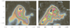 |
Fig. 10 Comparison of integrated line intensities of [C II] (color) and [O I] at 63 μm (contour) over different velocity ranges. Shown on the left is the blue velocity component between −19 and −14 km s−1 and on the right, the red velocity component between −13 and −10 km s−1. The filled, red asterisk shows the position of CPD −59°2661. The positional offsets are relative to the center α = 10h45m55.s05,δ = –59d57m16.′′7 (J2000). |
5 Discussion
We compare the high spatial resolution (7′′) velocity-resolved observations of the [O I] at 63 μm lines in G287.84-0.82 with the [C II], CO (and its isotopologs) and H2CO to understand the small-scale structure of the PDR created by the embedded Treasure Chest cluster. As shown in Fig. 4 the emission from the region has clearly blue- and red-shifted components. Figure 10 compares the emission in the blue (υLSR = −19 to −14 km s−1) and red (υLSR = −13 to −10 km s−1) parts of the spectrum. In the blue part we find [O I] tracing out mostly the higher-density regions including the PDR surface to the southwest of the main pillar. The same is seen in [C II], which additionally is seen in the tail regions of the globule. The overlay of red-shifted [C II] and [O I] emission also match very well, suggesting the PDR shell surrounding CPD −59°2661 is dominantly at this velocity. The eastern, red-shifted tail of the globule is strong in both [C II] and [O I], while the middle tail is only seen in [C II], suggesting that it has lower densities. The western pillar (the duck head) clearly stands out in the high spatial resolution [O I] data and is seen in [C II] as well. It appears to have about the same velocity as the main pillar. The head is seen in CO(11–10) as well.
The higher spatial resolution [O I] data resolve the PDR shell around the Treasure Chest cluster, with the semi-shell being easily seen in the red-shifted [O I] image. This is also consistent with our [C II] data. There is little overlap between the peaks in the blue- and red-shifted emission, which is consistent with an expanding shell. The northeastern part is somewhat blue-shifted, while the emission is more red-shifted to the west. The red- and the blue-shifted components of [C II] and [O I] emission differ in velocity by ~ 4 km s−1. This is muchsmaller than the velocity split seen in Hα, 25 km s−1, toward CPD −59°2661 by Walsh (1984). Although Walsh (1984) interpreted it as a measure of the expansion velocity (12 km s−1) of the nebula, he noted that “there is no evidence for the split components gradually joining up to the velocity of the adjacent material, as might be expected for a shell.” Our observations show that the expansion velocity is only ~ 2 km s−1, hence the dynamical age of the H II region (a few times 104 yr, as concluded by Smith et al. 2005) is severely underestimated. In order for the H II region to expand into the surrounding dense molecular-cloud, a more realistic estimate of the age is ~ 1 Myr, which is in good agreement with the age of the cluster, 1.3 Myr, as estimated by Oliveira et al. (2018).
5.1 The PDR gas
To some degree we can distinguish the emission from the diffuse and dense components of the gas by looking at the emission in different velocity intervals. Thus, if we compare the intensities due to the blue-shifted [C II] and CO(2–1) emission from the eastern tail with PDR models, it will be possible to derive an estimate of the density of the diffuse gas. Additionally, we used the line intensities of [O I] and CO(11–10), both of which are high-density PDR tracers, at the positions of the intensity peaks of [O I] seen clearly in the shell around the embedded cluster (Fig. 10).
In order to estimate the physical conditions in the dense and diffuse PDR in the cloud surrounding the Treasure Chest nebula, we compared the observed line-intensity ratios with the results of the model for PDRs by Kaufman et al. (1999). These models consider a semi-infinite slab of constant density, which is illuminated by far-ultraviolet (FUV) photons from one side. The model includes the major heating and cooling processes and incorporates a detailed chemical network. Comparison of the observed intensities with the steady-state solutions of the model helps to determine the gas density of H nuclei, nH, and the FUV flux (6 eV ≤ hν < 13.6 eV), G0, measured in units of the Habing (1968) value for the average solar neighborhood FUV flux, 1.6 × 10⁻³ ergs cm−2 s−1.
Since the PDR inside the Treasure Chest cloud is created by the embedded cluster, the strength of the FUV radiation in the region can be estimated from the total far-infrared (FIR) intensity observed, by assuming that FUV energy absorbed by the grains is reradiated in the FIR. Based on this method, Roccatagliata et al. (2013) derived the FUV map for the region using PACS and SPIRE dust continuum observations, with the values of FUV radiation field lying between 900 and 5000 times G0, where G0 is in units of the Habing field. From their FUV map (Fig. 7 in Roccatagliata et al. 2013), we estimate the FUV intensity to be around 1000 G0 in the eastern tail and around 5000 G0 in the region where the PDR shell is detected.
In order to compare the observed intensity ratios of [C II]/ CO(11–10), [O I]/CO(11–10), [O I]/[C II], and [C II]/CO(2–1) for the dense gas with PDR models, we compared emission arising in the same velocity range for the tracers involved in a particular ratio. Since among all the tracers [C II] is the broadest at most positions, we first fitted a single-component Gaussian profile to the spectrum of the other tracer in the ratio. Subsequently we fitted a Gaussian profile with identical central velocity and full width half maximum (FWHM) to obtain the velocity-integrated line-intensity for [C II]. In order to do this position-by-position analysis, we spatially regridded the datacubes corresponding to a particular ratio to the grid of the cube with lower resolution. Thus the analysis is restricted to around 300 positions where such fits were possible. We find that the intensity ratios (in energy units) [C II]/CO(11–10), [C II]/CO(2–1), and [O I]/[C II] range between 10–70, 50–450, and 3–7 respectively for these positions. For the [O I]/CO(11–10), we fit the CO(11–10) spectra first and then used the same parameters to extract the intensity of the [O I] spectrum. The [O I]/CO(11–10) intensity ratio is thus estimated to range between 30 and 210. For the diffuse gas traced only by [C II] and CO(2–1), we used the ratio of intensities of [C II] and CO(2–1) between −18 and −14 km s−1 in the eastern tail region, where no [O I] emission is seen at these velocities. The CO(2–1) intensities are estimated from the observed intensities of the optically thin 13CO(2–1) spectra. The [C II]/CO(2–1) ratio for the eastern tail ranges between 1000 and 2000 (in energy units).
Figure 11 shows results of comparison of the observed intensity ratios with the predictions of the PDR models. The two horizontal lines correspond to 1000 and 5000 G0 for the western tail and the PDR shell around the cluster. For each intensity ratio two contours are drawn to indicate the range of observed values. We assumed that the beam-filling factors of the different PDR tracers are identical so that the line-intensity ratios considered here are independent of the beam-filling.
The observed [C II]/CO(2–1) ratios for the diffuse gas in the eastern tail are consistent with n(H) between 600 and 2200 cm−3. For the denser gas the [C II]/CO(2–1) suggest a somewhat wider range of values between 104 and 106 cm−3. The [C II]/CO(11–10) primarily estimated in the head of the globule suggest a narrower range of densities between (0.8–1.6) × 105 cm−3. The [O I]/CO(11–10) ratio with both high-density tracers suggests densities between (2–8) × 105 cm−3. The [O I]/[C II] ratio estimated for positions spanning both the head and tails of the globule suggests densities between 2 × 10³–1.8 × 104 cm−3. The much lower densities suggested by the [O I]/[C II]/ ratio indicate that the [C II] emission is dominated by lower density, more diffuse PDR gas.
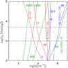 |
Fig. 11 Contours of observed intensity ratios plotted on the intensity predictions as a function of hydrogen density nH and FUV radiation field (G0) from PDR models for the selected regions in the cloud around Treasure Chest. The horizontal dashed lines correspond to FUV in the eastern tail (1000 G0) and close to the embedded cluster (5000 G0), as estimated by Roccatagliata et al. (2013). The contours of [C II]/CO(2–1) (green), [C II]/CO(11–10) (brown), [O I]/CO(11–10) (blue), and [O I]/[C II] (red) correspond to the extreme values that these ratios (see text) take up. The ratios are inenergy units. |
5.2 Thermal pressure in the region
Based on the analysis of the tracers of molecular and PDR gas of different densities, we identify several temperature components in the G287.84-0.82 globule. The first component corresponds to the temperature of the molecular gas, which is estimated to be ~ 40 K based on the observed peak temperatures of CO(2–1). The second component corresponds to PDR gas at a temperature of 100 K, as derived from the analysis of [13C II] intensities. Additionally, the high-density (~ 105 cm−3) molecular gas emitting in H2CO show average kinetic temperatures of 60–70 K within a limited region in the head of the globule. It is likely that a fourth component with densities of ~ 600–2200 cm−3 and of less well-determined temperature exists in the tail regions.
From analysis of [O I] and CO(11–10) using PDR models we determined that densities of dense PDR gas lie between (2–8) × 105 cm−3. For typical PDR temperatures of 100–300 K, this corresponds to a thermal pressure of 2 × 10⁷–2.4 × 10⁸ K km s−1. Ratios of intensities involving [C II] suggest densities around 104 cm−3 for the diffuse PDR gas, which for a temperature of 100 K corresponds to a thermal pressure of 106 cm−3. The global pressure of the molecular gas traced by CO(2–1) with a density of ~ 104 cm−3 and Tkin = 40 K, corresponds to 4 × 10⁵ K cm−3. If we consider the diffuse PDR gas in the eastern tails with densities between 600 and 2200 cm−3 to have thermal pressure (Pth) of the same order as the cold molecular gas, then the temperature of the gas would correspond to temperatures exceeding 200 K.
The sharp contrast in estimated thermal pressure of the diffuse and dense phases of PDR gas in the region is similar to the results of Stock et al. (2015), where two phases with pressures of 105 and 108 K cm−3 were detected in multiple sources. It is also similar to the results of Wu et al. (2018), who estimate Pth~ 108 K cm−3 across the dissociation front in Car I-E region. Wu et al. (2018) also suggested an empirical relationship 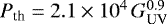 between the UV field and thermal pressure. For GUV ~ 5000 G0 for the dense regions, Pth will be ~ 4 × 10⁷ K cm−3, which is approximately consistent with the Pth we derived from the n(H2) and Tkin.
5.3 Possible triggered star formation in the Treasure Chest
Although it is clear that star formation can be triggered in cometary globules (Lefloch et al. 1997; Ikeda et al. 2008; Mookerjea & Sandell 2009), this is not the case for the Treasure Chest cluster. There are 19 OB clusters in the Carina nebula (Tapia et al. 2003; Smith 2006; Oliveira et al. 2018). Even though the Treasure Chest is one of the youngest, 1.3 Myr (Oliveira et al. 2018), it is still too old to have been triggered by the formation of the cometary globule. It is far more likely that the Treasure Chest had already formed before G287.84 became a cometary globule, and subsequently became a dense, massive cloud-core surrounded by lower density gas. When the Carina H II region expanded, it blew away the lower density gas, first creating a giant pillar, which later became the cometary globule that we see today. Although the cometary globule continues to be eroded by the stellar winds from η Car and Trumpler 16, the expanding H II region from the Treasure Chest cluster appears to erode it even faster. It has already expanded through the western side of the globule and most of the molecular cloud is already gone on the northwestern side as well. There is, however enough dense gas, ~1000 M⊙, to collapse and form stars. However, it is likely that the time scale for star formation is longer than the time it takes for the globule to be evaporated by the FUV radiation from the Treasure Chest cluster, as well as by the FUV radiation from η Car and the O stars in Trumpler 16.
The heavily reddened young star, 2MASS J10453974-5957341 in the duck head, could be a case of triggered star formation. However, it is more likely that it formed about the same time the Treasure Chest cluster formed, and is therefore presumably a member of the Treasure Chest cluster.
6 Summary
We used velocity-resolved observations of various tracers of (i) PDR ([O I], [C II], CO(11–10)), (ii) ambient molecular material (J = 2–1 transitions of CO, 13CO, and C18O), and (iii) high-density gas (H2CO and SO) to study detailed physical and velocity structures of the G287.84-0.82 cometary globule in Carina. The high quality of [C II] data enabled simultaneous detection of the F = 2–1 transition of the rarer isotope of C+ and subsequent determination of N(C+) ~ 0.3–1 × 1019 cm−2. We conclude that the overall structure of the source including its velocities is consistent with the globule being sculpted by the radiation and winds of the nearby OB associations in Trumpler 16 and η Carina. As revealed with enhanced clarity by the higher spatial resolution (7′′) [O I] data, the details of the distribution of PDR gas inside the globule are consistent with illumination by CPD −59°2661 the brightest member of the Treasure chest cluster. The density and temperature of the PDR gas, estimated to consist of a diffuse and a dense part were determined using observed line-intensity ratios in combination with non-LTE radiative transfer models as well as plane-parallel PDR models. We identified at least two components of PDR gas with densities of 104 and (2–8) × 105 cm−3. Based on temperatures estimated, the thermal pressure in the diffuse and dense PDR components are 106 and 107 –108 K cm−3, respectively. This contrast in thermal pressure of the diffuse and dense phases of PDR gas is similar to the findings that exist in the literature.
Acknowledgements
Based in part on observations made with the NASA/DLR Stratospheric Observatory for Infrared Astronomy (SOFIA). SOFIA is jointly operated by the Universities Space Research Association, Inc. (USRA), under NASA contract NNA17BF53C, and the Deutsches SOFIA Institut (DSI) under DLR contract 50 OK 0901 to the University of Stuttgart.
Appendix A Additional channel maps
Here we show channel maps of CO(11–10), 2–1 transitions of CO (and isotopologs), H2CO(303–202) and SO(65 → 54).
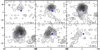 |
Fig. A.1 Velocity channel maps of CO(11–10) of G287.84. |
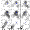 |
Fig. A.2 Velocity channel maps of CO(2–1) G287.84. |
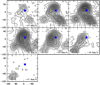 |
Fig. A.3 Velocity channel maps of 13CO(2–1) of G287.84. |
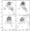 |
Fig. A.4 Velocity channel maps of C18O(2–1) of G287.84. |
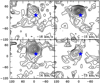 |
Fig. A.5 Velocity channel maps of H2CO(303–202). |
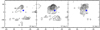 |
Fig. A.6 Velocity channel maps of SO(65 → 54). |
References
- Bertoldi, F. 1989, ApJ, 346, 735 [NASA ADS] [CrossRef] [Google Scholar]
- Bertoldi, F., & McKee, C. F. 1990, ApJ, 354, 529 [NASA ADS] [CrossRef] [Google Scholar]
- Bisbas, T. G., Wünsch, R., Whitworth, A. P., Hubber, D. A., & Walch, S. 2011, ApJ, 736, 142 [Google Scholar]
- Breen, S. L., Green, C. -E., Cunningham, M. R., et al. 2018, MNRAS, 473, 2 [NASA ADS] [CrossRef] [Google Scholar]
- de Graauw, T., Lidholm, S., Fitton, B., et al. 1981, A&A, 102, 257 [NASA ADS] [Google Scholar]
- Frerking, M. A., Langer, W. D., & Wilson, R. W. 1982, ApJ, 262, 590 [NASA ADS] [CrossRef] [Google Scholar]
- Gagné, M., Fehon, G., Savoy, M. R., et al. 2011, ApJS, 194, 1 [NASA ADS] [CrossRef] [EDP Sciences] [Google Scholar]
- Ghosh, S. K., Iyengar, K. V. K., Rengarajan, T. N., et al. 1988, ApJ, 330, 928 [NASA ADS] [CrossRef] [Google Scholar]
- Guan, X., Stutzki, J., Graf, U., et al. 2012, A&A, 542, L4 [NASA ADS] [CrossRef] [EDP Sciences] [Google Scholar]
- Güsten, R., Nyman, L. Å., Schilke, P., et al. 2006, A&A, 518, L79 [Google Scholar]
- Habing, H. J. 1968, Bull. Astron. Inst. Netherlands, 19, 421 [Google Scholar]
- Hägele, G. F., Albacete Colombo, J. F., Barbá, R. H., et al. 2004, MNRAS, 355, 1237 [NASA ADS] [CrossRef] [Google Scholar]
- Hartigan, P., Reiter, M., Smith, N., & Bally, J. 2015, AJ, 149, 101 [NASA ADS] [CrossRef] [Google Scholar]
- Harvey, P. M., Hoffmann, W. F., & Campbell, M. F. 1979, ApJ, 227, 114 [NASA ADS] [CrossRef] [Google Scholar]
- Heyminck, S., Graf, U. U., Güsten, R., et al. 2012, A&A, 542, L1 [NASA ADS] [CrossRef] [EDP Sciences] [Google Scholar]
- Ikeda, H., Sugitani, K., Watanabe, M., et al. 2008, AJ, 135, 2323 [NASA ADS] [CrossRef] [Google Scholar]
- Kaufman, M. J., Wolfire, M. G., Hollenbach, D. J., & Luhman, M. L. 1999, ApJ, 527, 795 [NASA ADS] [CrossRef] [Google Scholar]
- Klein, B., Hochgürtel, S., Krämer, I., et al. 2012, A&A, 542, L3 [NASA ADS] [CrossRef] [EDP Sciences] [Google Scholar]
- Langer, W. D., Goldsmith, P. F., Pineda, J. L., et al. 2018, A&A, 617, A94 [NASA ADS] [CrossRef] [EDP Sciences] [Google Scholar]
- Lefloch, B., & Lazareff, B. 1994, A&A, 289, 559 [NASA ADS] [Google Scholar]
- Lefloch, B., Lazareff, B., & Castets, A. 1997, A&A, 324, 249 [NASA ADS] [Google Scholar]
- Mangum, J. D., & Wootten, A. 1993, ApJS, 89, 123 [NASA ADS] [CrossRef] [Google Scholar]
- Mookerjea, B., & Sandell, G. 2009, ApJ, 706, 896 [NASA ADS] [CrossRef] [Google Scholar]
- Mookerjea, B., Sandell, G., Vacca, W., Chambers, E., & Güsten, R. 2018, A&A, 616, A31 [NASA ADS] [CrossRef] [EDP Sciences] [Google Scholar]
- Oliveira, R. A. P., Bica, E., & Bonatto, C. 2018, MNRAS, 476, 842 [NASA ADS] [CrossRef] [Google Scholar]
- Ossenkopf, V., Röllig, M., Neufeld, D. A., et al. 2013, A&A, 550, A57 [NASA ADS] [CrossRef] [EDP Sciences] [Google Scholar]
- Rathborne, J.M., Brooks, K. J., Burton, M. G., et al. 2004, A&A, 418, 563 [NASA ADS] [CrossRef] [EDP Sciences] [Google Scholar]
- Rebolledo, D., Burton, M., Green, A., et al. 2016, MNRAS, 456, 2406 [NASA ADS] [CrossRef] [Google Scholar]
- Risacher, C., Güsten, R., & Stutzki, J., et al. 2016, A&A, 595, A34 [NASA ADS] [CrossRef] [EDP Sciences] [Google Scholar]
- Roccatagliata, V., Preibisch, T., Ratzka, T., & Gaczkowski, B. 2013, A&A, 554, A6 [NASA ADS] [CrossRef] [EDP Sciences] [Google Scholar]
- Sault, R. J., Teuben, P. J., & Wright, M. C. H. 1995, in Astronomical Data Analysis Software and Systems IV, eds. R. A. Shaw, H. E. Payne, & J. J. E. Hayes, ASP Conf. Ser., 77, 433 [NASA ADS] [Google Scholar]
- Schneider, N., Ossenkopf, V., Csengeri, T., et al. 2015, A&A, 575, A79 [NASA ADS] [CrossRef] [EDP Sciences] [Google Scholar]
- Schöier, F. L., van der Tak, F. F. S., van Dishoeck, E. F., & Black, J. H. 2005, A&A, 432, 369 [NASA ADS] [CrossRef] [EDP Sciences] [Google Scholar]
- Shirley, Y. L. 2015, PASP, 127, 299 [NASA ADS] [CrossRef] [Google Scholar]
- Smith, N. 2004, MNRAS, 351, L15 [NASA ADS] [CrossRef] [Google Scholar]
- Smith, N. 2006, MNRAS, 367, 763 [NASA ADS] [CrossRef] [Google Scholar]
- Smith, N., Egan, M. P., Carey, S., et al. 2000, ApJ, 532, L145 [NASA ADS] [CrossRef] [PubMed] [Google Scholar]
- Smith, N., Stassun, K. G., & Bally, J. 2005, AJ, 129, 888 [NASA ADS] [CrossRef] [Google Scholar]
- Smith, N., Povich, M. S., Whitney, B.A., et al. 2010, MNRAS, 406, 952 [NASA ADS] [Google Scholar]
- Stock, D. J., Wolfire, M. G., Peeters, E., et al. 2015, A&A, 579, A67 [NASA ADS] [CrossRef] [EDP Sciences] [Google Scholar]
- Sugitani, K., Tamura, M., Nakajima, Y., et al. 2002, ApJ, 565, L25 [NASA ADS] [CrossRef] [Google Scholar]
- Tapia, M., Roth, M., Vázquez, R. A., et al. 2003, MNRAS, 339, 44 [NASA ADS] [CrossRef] [Google Scholar]
- Thackeray, A. D. 1950 MNRAS, 110, 524 [NASA ADS] [Google Scholar]
- van der Tak, F. F. S., Black, J. H., Schoïer, F. L., Jansen, D. J., & van Dishoeck, E. F. 2007, A&A, 468, 627 [NASA ADS] [CrossRef] [EDP Sciences] [Google Scholar]
- Walsh, J. R. 1984, A&A, 138, 380 [NASA ADS] [Google Scholar]
- Wamsley, C. M., & Ungerechts, H. 1983, A&A, 122, 164 [NASA ADS] [Google Scholar]
- White, G. J., & Sandell, G. 1995, A&A, 299, 179 [NASA ADS] [Google Scholar]
- Wiesenfeld, L., & Faure, A. 2013, MNRAS, 432, 2573 [NASA ADS] [CrossRef] [Google Scholar]
- Wu, R., Bron, E., Onaka, T., et al. 2018, A&A, 618, A53 [NASA ADS] [CrossRef] [EDP Sciences] [Google Scholar]
- Young, E. T., Becklin, E. E., Marcum, P. M., et al. 2012, ApJ, 749, L17 [NASA ADS] [CrossRef] [Google Scholar]
The development of GREAT was financed by the participating institutes, by the Federal Ministry of Economics and Technology via the German Space Agency (DLR) under Grants 50 OK 1102, 50 OK 1103 and 50 OK 1104 and within the Collaborative Research Centre 956, sub-projects D2 and D3, funded by the Deutsche Forschungsgemeinschaft (DFG).
CLASS is part of the Grenoble Image and Line Data Analysis Software (GILDAS), which is provided and actively developed by IRAM, and is available at http://www.iram.fr/IRAMFR/GILDAS
APEX, the Atacama Pathfinder Experiment is a collaboration between the Max-Planck-Institut für Radioastronomie at 55%, Onsala Space Observatory (OSO) at 13%, and the European Southern Observatory (ESO) at 32% to construct and operate a modified ALMA prototype antenna as a single dish on the high altitude site of Llano Chajnantor. The telescope was manufactured by VERTEX Antennentechnik in Duisburg, Germany.
For 13CO(2–1) we created a map with a pixel size of 9″.5 × 9″.5, as in one third of a HPBW.
All Tables
Results of single (or double for position #8) component Gaussian fitting of observed spectra.
All Figures
|
Fig. 1 Spitzer IRAC 8 μm image of South Pillars of Carina showing the location of the Treasure Chest region on a larger perspective. The image artifacts from the exceedingly bright O2 star η Carina, marked by a star symbol, completely hides the massive OB cluster, Trumpler 16, located just southwest of it. The G287.84 pillar is shown with a rectangle. |
| In the text | |
|
Fig. 2 Spitzer 8 μm image of the cometary globule G287.84-0.82. One can see three tails extending to the south from the head part of the globule. All tails point away from η Car and the O stars in Trumpler 16, which are to the northwest of the globule, see Fig. 1. The internal PDR, illuminated by CPD −59°2661 in the Treasure Chest cluster, is seen as a bright semi-shell in the northern part of the image. A secondary pillar, which we call the “duck head”, is west of the Treasure Chest cluster. It also has an embedded young star in the head. Faint foreground PDR emission is seen all around the globule, especially to the north. We have marked the position of CPD −59°2661 and Hen 3-485. The two dashed lines indicate the cuts for position–velocity plots discussed later in the text. The extraction positions of spectra discussed in Sect. 3 are labeled 1–8. |
| In the text | |
|
Fig. 3 Contours of intensity integrated between −20 and −5 km s−1 of [C II] (black contour) overlayed on false-color images of tracers mentioned in the panels. Top row: tracers of PDR gas, middle row: tracers of high-density gas, bottom row: tracers of overall gas and dust distribution in the region. The filled asterisk shows the position of CPD −59°2661. The color scale for each panel is shown next to the panel and the units are K km s−1 for the spectral lines, MJy sr−1 for 8 μm and Jy pixel−1 for PACS (3′′ pixel). The values of [C II] contours are 10–100% of the peak intensity of 505 K km s−1. |
| In the text | |
|
Fig. 4 Channel maps of [C II] (top) and [O I] 63 μm (bottom) emission. Velocities corresponding to the channel are marked in each panel. The red star marks the position of CPD −59°2661. The positional offsets are relative to the center α = 10h45m55.s05, δ = −59d57m16.′′7 (J2000). |
| In the text | |
|
Fig. 5 Comparison of emission spectra of [C II] (filled histogram), 13CO(2–1) (red), CO(11–10) (green), and [O I] 63 μm (black) at selected positions shown in panel 2 of Fig. 3. The 13CO, CO(11–10), and [O I] spectra are multiplied by factors of 4, 2, and 3, respectively. |
| In the text | |
|
Fig. 6 Spectra of the J = (303–202), (322 –221), and (321–220) transitions of para-H2CO at selected positions where the fainter lines are clearly detected. |
| In the text | |
|
Fig. 7 Examples of [C II] spectra at two positions where [13C II] is also detected. The emission feature at approximately −28 km s−1 is from faint foreground PDR emission unrelated to the globule. The lower panels show an expanded view of the [13C II] lines, along with the result of simultaneous fitting of [C II] and [13C II] lines as describedin the text. |
| In the text | |
|
Fig. 8 RADEX non-LTE modeling of 303–202/321–220 ratio of H2CO. The ratio is calculated as a function of the gas kinetic temperature (Tkin) and column density of H2CO for the volume densities n(H2) of 105 (left) and 106 cm−3 (right). Contours with labels mark the observed line-intensity ratios for H2CO. |
| In the text | |
|
Fig. 9 Position–velocity plots of [C II], [O I], and 13CO(2–1) in contours enhanced with gray-scale along cuts shown in Fig. 2. The zero position for the NW-SE cut (top panels) is at (+27′′,−23″. 5) and for the NE-SW cut (bottom panels) at (−27′′,+10′′), relative to the map center. For each cut we plotted 10 contours. For [C II] these go from 1.4 K to peak temperature. For [O I] and 13CO(2–1) the lowest contours are 3 and 0.4 K, respectively. The gray-scale goes from zero to 1.5 times the peak temperature. For all cuts we drew the position of the PDR rims (as seen in 8 μm IRAC image) with a dotted line, as well as the position of the ionizing star, CPD −59°2661. The rims and the O star are labeled in the middle panel. In the NE-SW cut the dotted line labeled “neck” indicates the middle of the duck neck. |
| In the text | |
|
Fig. 10 Comparison of integrated line intensities of [C II] (color) and [O I] at 63 μm (contour) over different velocity ranges. Shown on the left is the blue velocity component between −19 and −14 km s−1 and on the right, the red velocity component between −13 and −10 km s−1. The filled, red asterisk shows the position of CPD −59°2661. The positional offsets are relative to the center α = 10h45m55.s05,δ = –59d57m16.′′7 (J2000). |
| In the text | |
|
Fig. 11 Contours of observed intensity ratios plotted on the intensity predictions as a function of hydrogen density nH and FUV radiation field (G0) from PDR models for the selected regions in the cloud around Treasure Chest. The horizontal dashed lines correspond to FUV in the eastern tail (1000 G0) and close to the embedded cluster (5000 G0), as estimated by Roccatagliata et al. (2013). The contours of [C II]/CO(2–1) (green), [C II]/CO(11–10) (brown), [O I]/CO(11–10) (blue), and [O I]/[C II] (red) correspond to the extreme values that these ratios (see text) take up. The ratios are inenergy units. |
| In the text | |
|
Fig. A.1 Velocity channel maps of CO(11–10) of G287.84. |
| In the text | |
|
Fig. A.2 Velocity channel maps of CO(2–1) G287.84. |
| In the text | |
|
Fig. A.3 Velocity channel maps of 13CO(2–1) of G287.84. |
| In the text | |
|
Fig. A.4 Velocity channel maps of C18O(2–1) of G287.84. |
| In the text | |
|
Fig. A.5 Velocity channel maps of H2CO(303–202). |
| In the text | |
|
Fig. A.6 Velocity channel maps of SO(65 → 54). |
| In the text | |
Current usage metrics show cumulative count of Article Views (full-text article views including HTML views, PDF and ePub downloads, according to the available data) and Abstracts Views on Vision4Press platform.
Data correspond to usage on the plateform after 2015. The current usage metrics is available 48-96 hours after online publication and is updated daily on week days.
Initial download of the metrics may take a while.