| Issue |
A&A
Volume 625, May 2019
|
|
|---|---|---|
| Article Number | A57 | |
| Number of page(s) | 11 | |
| Section | Stellar atmospheres | |
| DOI | https://doi.org/10.1051/0004-6361/201834850 | |
| Published online | 10 May 2019 | |
The Galactic WN stars revisited
Impact of Gaia distances on fundamental stellar parameters
1
Institut für Physik und Astronomie, Universität Potsdam,
Karl-Liebknecht-Str. 24,
14476
Potsdam,
Germany
e-mail: This email address is being protected from spambots. You need JavaScript enabled to view it.
2
Argelander-Institut für Astronomie der Universität Bonn,
Auf dem Hügel 71,
53121
Bonn,
Germany
3
Leibniz-Institut für Astrophysik (AIP),
An der Sternwarte 16,
14482
Potsdam,
Germany
4
Armagh Observatory and Planetarium,
College Hill,
Armagh,
BT61 9DG,
UK
5
Institute of Astrophysics, KU Leuven,
Celestijnenlaan 200 D,
3001 Leuven,
Belgium
6
Kazan Federal University,
Kremlevskaya Ul. 18,
Kazan,
Russia
Received:
13
December
2018
Accepted:
27
March
2019
Abstract
Comprehensive spectral analyses of the Galactic Wolf-Rayet stars of the nitrogen sequence (i.e. the WN subclass) have been performed in a previous paper. However, the distances of these objects were poorly known. Distances have a direct impact on the “absolute” parameters, such as luminosities and mass-loss rates. The recent Gaia Data Release (DR2) of trigonometric parallaxes includes nearly all WN stars of our Galactic sample. In the present paper, we apply the new distances to the previously analyzed Galactic WN stars and rescale the results accordingly. On this basis, we present a revised catalog of 55 Galactic WN stars with their stellar and wind parameters. The correlations between mass-loss rate and luminosity show a large scatter, for the hydrogen-free WN stars as well as for those with detectable hydrogen. The slopes of the log L − log Ṁ correlations are shallower than found previously. The empirical Hertzsprung–Russell diagram (HRD) still shows the previously established dichotomy between the hydrogen-free early WN subtypes that are located on the hot side of the zero-age main sequence (ZAMS), and the late WN subtypes, which show hydrogen and reside mostly at cooler temperatures than the ZAMS (with few exceptions). However, with the new distances, the distribution of stellar luminosities became more continuous than obtained previously. The hydrogen-showing stars of late WN subtype are still found to be typically more luminous than the hydrogen-free early subtypes, but there is a range of luminosities where both subclasses overlap. The empirical HRD of the Galactic single WN stars is compared with recent evolutionary tracks. Neither these single-star evolutionary models nor binary scenarios can provide a fully satisfactory explanation for the parameters of these objects and their location in the HRD.
Key words: stars: mass-loss / stars: winds, outflows / stars: Wolf-Rayet / stars: atmospheres / stars: evolution / stars: distances
© ESO 2019
1 Introduction
Massive stars play an essential role in the Universe. With their feedback of ionizing photons and their stellar mass loss, these stars govern the ecology of their extended neighborhood. Their final gravitational collapse is probably in most cases accompanied by a supernova explosion or even gamma-ray burst. In case a close pair of compact objects (neutron stars or black holes) is left over, these compact remnants will spiral in over gigayears until they finally merge with a spectacular gravitational wave event as those detected in the recent years.
Many massive stars will pass through Wolf-Rayet (WR) stages in advanced phases of their evolution. However, these last stages of massive-star evolution are yet poorly understood. Major uncertainties are induced by the lack of knowledge in various aspects: the stellar mass loss in the O-star phase and in the WR phase(s) (e.g., Mokiem et al. 2007; Hainich et al. 2015); eruptive mass-loss (e.g., luminous blue variables; Smith & Owocki 2006); mass loss in the red supergiant stage (Vanbeveren et al. 2007); angular momentum loss; internal mixing processes, including rotationally induced mixing (e.g., Maeder 2003); binary fraction (Sana 2017); close-binary evolution with mass exchange (e.g., Marchant et al. 2016); common-envelope evolution (Paczynski 1976); and stellar mergers. Complicating things even more, all these issues depend on the metallicity of the respective stars.
In this situation, it is crucial to establish empirical constraints. We previously analyzed a comprehensive sample of Galactic WN stars (Hamann et al. 2006, hereafter Paper I). This homogeneous set of spectral analyses was based on the Potsdam Wolf-Rayet (PoWR) model atmospheres1. This state-of-the-art non-LTE code solves the radiative transfer in a spherically expanding atmosphere and accounts not only for complex model atoms, but also for iron line blanketing and for wind clumping (Gräfener et al. 2002; Hamann & Gräfener 2004).
A basic disadvantage of the Galactic WN sample was the large uncertainty of the stellar distances. While the basic spectroscopic parameters (especially the stellar temperature T* and the “transformed radius” Rt; see Sect. 4) do not depend on the adopted distance, the “absolute” parameters (luminosity L, mass-loss rate Ṁ) do.
This situation fundamentally improved with the recent Gaia Data Release 2 (DR2). Fortunately, WR spectra closely follow a scaling invariance, which makes it possible to rescale the results from Paper I to the new Gaia distances without redoing the whole spectral analyses. This is the core of the present paper. The same task has already been carried out for the Galactic WC and WO stars (Sander et al. 2019). Naturally, our analyses of WR stars in the Magellanic Clouds (Hainich et al. 2014, 2015; Shenar et al. 2016, 2018) or in M 31 (Sander et al. 2014) do not suffer from distance uncertainties.
The rest of the paper is structured as follows. In Sect. 2 we introduce our sample and review the binary status. In Sect. 3 we adapt the Gaia DR2 parallaxes and distances for our sample, and investigate the impact of the revised distances on the WN star positions in the Galaxy and on their absolute visual magnitudes. Section 4 describes the rescaling of the stellar parameters from Paper I, while the results of this procedure are visualized in Sect. 5; especially, the updated Hertzsprung–Russell diagram (HRD) is discussed with regard to the evolutionary connections. A summary is given in the last section (Sect. 6).
2 The sample of WN stars
The present study relies on the same stars as Paper I (cf. Table 1). The list of objects analyzed in Paper I comprises the vast majority of Galactic WN stars that can be observed in visual light since they are not obscured too much by interstellar absorption. We left out those WN stars that show composite spectra, typically as WR+OB binaries. The concern at this point is that composite spectra need to be analyzed as such; neglecting their composite nature would compromise the results. Analyzing composite spectra is of course also manageable (see, e.g., Shenar et al. 2018, 2017, 2016), but requires more and better observational data and has been beyond the scope of Paper I.
In orderto make sure that the sample does not contain composite spectra with a significant contribution from the non-WR component, we checked the literature that has appeared since publication of Paper I. Below, we comment on the binary status of the individual stars in cases in which new evidence has been published.
WR 1 is still considered to be single; the observed polarization is attributed to corotating interaction regions (CIRs) rather than to wind asymmetry (St-Louis 2013).
WR 2 has been extensively observed by Chené et al. (2019), who did not find any evidence for binarity. These authors identified only a small contribution (5%) to the optical spectrum by a B-type star in the background with a projected distance of 0.′′25.
WR 6 is still considered to be single; the polarimetric and photometric variability was rediscussed by St-Louis et al. (2018) and attributed to CIRs.
WR 12 is clearly a binary with colliding winds; however, no traces of the putative OB-type companion could be identified in the spectrum (Fahed & Moffat 2012), indicating that its contribution is minor.
WR 22 is clearly a WR+O binary; Rauw et al. (1996) estimated that the O-type companion is about eight times fainter than the WR primary (at 5500 Å). Thus, neglecting the contribution of the O star should introduce only a limited bias on the spectral analysis.
WR 25 shows an X-ray light curve with a period of 208 d, confirming a WR+O colliding wind system (Pandey et al. 2014). Its eccentric orbit has been established first by Gamen et al. (2008), who claimed minimum masses of 75 + 27 M⊙, but did not report a brightness ratio. The distance to WR 25 has been revised significantly by Gaia, from DM = 12.55 mag (Paper I) to 11.5 mag corresponding to 2.0 kpc, which is nearer than the bulk of the Carina nebula.
WR 40 is unusually faint in X-rays, in contrast to the expectation that it could be a colliding-wind binary (Gosset et al. 2005).
WR 44 shows variability that is typical for CIRs rather than indicating binarity (Chené et al. 2011).
WR 47 was excluded from the sample of Paper I because of suspected composite spectrum. Meanwhile, it has been studied by Fahed & Moffat (2012) as a colliding-wind system. O-star features could not be identified in the spectrum, implying that the contribution of this component to the total light is small. Hence, we actually could have kept the spectrum in our single-star analysis. WR 47 is a runaway (Tetzlaff et al. 2011).
WR 66 has a negative parallax measurement in Gaia DR2, probably because the visual companion which is separated by 0.4′′ and 1.05 mag fainter was interfering with the astrometry.
WR 78 shows no evidence of binarity, although Skinner et al. (2012) note that its X-rays include a hot plasma component “at the high end of the range for WN stars”.
WR 89 is a thermal radio source (Montes et al. 2009), supporting the assumption that it is single.
WR 105 shows non-thermal radio emission (Montes et al. 2009), which could be indicative of colliding winds, but there are no other signs of binarity.
WR 107 got a negative parallax measurement in Gaia DR2 for unknown reasons.
WR 123 has been extensively monitored with MOST (Lefèvre et al. 2005) and showed no stable periodic signals that could be attributed to orbital modulation (periods above one day). A persistent signal with about 9.8 h period is likely related to pulsational instabilities as claimed by Dorfi et al. (2006), although their stability analysis is based on the wrong assumption of a hydrogen-rich envelope.
WR 124 has been reported by Moffat et al. (1982) to show radial velocity variations. These authors suggested that the star might be a binary hosting a compact object. However, Marchenko et al. (1998a) could not confirm these radial velocity variations. A period search in the photometric data from HIPPARCOS also remained without significant detection (Marchenko et al. 1998b). The star is very faint in X-rays (LX ~ 1031 erg s−1). Nevertheless, Toala et al. (2018) showed that a hypothetical compact companion might be hidden deep in the wind. So far, WR 124 must be considered as being single.
WR 130 got a negative parallax measurement in Gaia DR2 for unknown reasons.
WR 134 shows spectral variability with a period of 2.25 d, which has been revisited in a long observational campaign by Aldoretta et al. (2016) and attributed to CIRs rather than to binarity.
WR 136 is a runaway star (Tetzlaff et al. 2011).
WR 147 is obviously a binary system with colliding winds. Chandra resolved a pair of X-ray sources (Zhekov & Park 2010).High-resolution radio observations also resolved two components, the southern thermal source WR 147S (the WN 8 star), and a northern non-thermal source WR 147N with a mutual separation of 0.′′57 (Abbott et al. 1986; Moran et al. 1989; Churchwell et al. 1992; Contreras et al. 1996; Williams et al. 1997; Skinner et al. 1999). The binary system was also spatially resolved in the infrared and optical range with a separation of 0.′′64 (Williams et al. 1997; Niemela et al. 1998). According to the latter work, the companion is by a factor 7.3 fainter in the visual than the WN 8 primary. Hence, our single-star spectral analysis might be slightly biased by contributions from the secondary and the colliding-wind zone. Gaia DR2 obtained a negative parallax for this object, presumably because the multiplicity of the light source has irritated the measurements.
WR 148 had been suspected to host a compact companion (Marchenko et al. 1996). However, Munoz et al. (2017) identified O-star features in the composite spectrum, and thus established a binary system with components classified as WN 7h and O4-6 in a 4.3 d orbit. While the brightness ratio was not determined, we must be aware that our single-star analysis might be somewhat biased by the contribution of the companion. The Gaia DR2 catalog reports a negative parallax, but it seems unlikely that is was the close-binary nature of the object that has irritatedthemeasurements. With a height of about 800 pc above the Galactic plane, WR 148 is an extreme runaway object.
WR 156 shows radio emission with a thermal and a non-thermal contribution (Montes et al. 2009), but otherwise there are no indications of binarity.
In those figures that indicate results of our spectral analysis, we mark the confirmed WR+OB binaries by encircling their respective symbol. Runaway stars are marked in the same way since their fast motion is most likely the result of former binarity, after the companion exploded and became gravitationally unbound.
We emphasize that all distance-independent results from the spectral analyses in Paper I are retained for the present study – notably the stellar temperatures, “transformed radii” (cf. Sect. 4), and the detectability of atmospheric hydrogen. Paper I provides a discussion of the error margins. The spectral types given in Col. 2 of Table 1 are copied from Paper I as well. We note that some of the stars with “early” subtype numbers are designated as “(WNL)” in parentheses, while some of the stars with subtype numbers as high as 7 or 8 are still classified in parantheses as “(WNE-w)”, i.e., as early-type WN with weak lines. In Paper I (end of Sect. 3) we argued that such assignment corresponds better to the spectral appearance. Since the current paper only updates the distance-dependent quatities, we keep these spectral type assignments throughout the present paper, including the symbol coding in the diagrams.
Parameters of the Galactic single WN stars.
3 Gaia distances for the Galactic WN stars
One of the main objectives of the Gaia space craft is to measure stellar parallaxes all over our Galaxy (Gaia Collaboration 2016). The original Gaia DR2 catalog2 provides parallaxes for 1.8 billion stars, including all our targets except of WR 2 and WR 63.
Ideally, the distance d to a particular object is just the reciprocal of its parallax d = ϖ−1. However, the measured parallax has a statistical error. As consequence, the most likely value for the distance is not exactly the reciprocal parallax. Bailer-Jones et al. (2018) provided a version of the Gaia DR2 catalog in which the distances are derived from the parallaxes with the help of a Bayesian approach. This catalog also provides error margins for the distance that correspond to a confidence level that is equivalent to 1σ in a Gaussian distribution.
We decided to retrieve the distances of our targets from the Bailer-Jones et al. catalog, although we are aware that this approach is based on a general model of the stellar density in our Galaxy. Bailer-Jones et al. (2018) gives positive distances even for those five stars of our sample (WR 66, 107, 130, 147, and 148) for which the original Gaia measurements resulted in negative parallaxes. In these cases the Bailer-Jones et al. distances mainly reflect the adopted Galactic model, and we disregard these values. We checked that they would lead to spurious results for the stellar parameters. Moreover, there is one star in the sample, WR 115, for which Gaia gives an amazingly small distance of 570 pc, but with a huge 1σ error from 335 to 2006 pc; this is by far the largest error margin within the sample. This measurement leads to implausible stellar parameters, and is also disregarded in the rest of this paper.
As mentioned above, the distances from the Bailer-Jones et al. (2018) version of the Gaia catalog are obtained with a Bayesian appoach, for which a specific model for the stellar density in our Galaxy had been adopted. This prior might not necessarily apply to our targets; for example, WR stars might be concentrated in the spiral arms. However, the construction of a special priorfor WR stars bears the danger that the results would be biased toward the expectations. Therefore we refrain from such attempts.
The Bayesian approach leads systematically to lower distances than the reciprocal parallax. Fortunately, this effect only becomes noticeable at largest distances, and thus affects only a few of our targets. For a Bayesian distance modulus of 14 mag the difference is about 0.5 mag and thus comparable to the typical 1σ uncertainty; for the farthest star in our sample (WR 49), the inverse parallax yields a distance modulus of 16.1 mag instead of 15.0 mag from the Bayesian approach. Our conclusions do not depend critically on these uncertainties, as we have checked.
For a couple of our targets, the Gaia DR2 catalog gives a non-zero astrometric_excess_noise which indicates a poor fit to the astrometric measurements (Arenou et al. 2018; Lindegren et al. 2018). Such poor astrometric solution might compromise the parallaxmeasurement, although this is not always reflected by especially large error margins. We consider a non-zero astrometric_excess_noise as a warning that the trigonometric distance might be less reliable and indicate the corresponding stars in the figures by printing their names in slanted font. In Table 1 the letterbetween Cols. 9 and 10 coding for the availability of a Gaia distance is a lower case “g” in these cases. However, the results shown in the rest of the paper do not give the impression that the flagged stars are outliers regarding their distance-dependent parameters, and thus do not substantiate doubts on their parallaxes.
The Galactic positions of our sample stars with Gaia distances, neglecting their height over the Galactic plane, are plotted in Fig. 1. As to be expected, they closely indicate the nearby spiral arms.
Essential for the present paper are the new Gaia distances, which are given in Table 1 Col. 9 in form of the distance modulus,
 (1)
(1)
flagged with the subsequent letter “G” when available, together with the error margins as described above. For the few stars without Gaia distance, Table 1 repeats the D M values from Paper I, and the subsequent arrow indicates whether this distance was derived from some cluster or association membership (→) or from theadopted subtype calibration of the absolute visual magnitude (←); see Paper I for details. Anyhow, all stars without Gaia distances are disregarded in the rest of this paper.
Comparing the Gaia distances for our remaining sample (55 stars) with those adopted in Paper I reveals a mild tendency to smaller values. The arithmetic mean over all distance moduli became lower by 0.2 mag, which corresponds to 10% smaller distances on average. However, for certain WN stars the D M values differsignificantly. Revisions of the distance modulus by more than 1.5 mag are encountered for WR 16 (ΔD M=1.5 mag), WR 82 (−2.6 mag), WR 83 (−2.6 mag), WR 120 (−1.7 mag), and WR 123 (−1.9 mag).
Photometry for WR stars is preferably considered in terms of the narrowband magnitudes defined by Smith (1968), using lower case letter subscripts (e.g., Mv, Mb) to distinguish them from Johnson broad-band colors. Adopting the same apparent magnitudes as in Paper I, and also keeping for each star the same reddening law and the same value for the color excess as in Paper I, the absolute visual magnitude Mv changes just by ΔD M due to the Gaia revision of the distance modulus.
The resulting absolute narrowband v magnitudes of our sample stars are plotted in Fig. 2 versus their WN subtype. In Paper I we had to rely on the assumption that there are strict correlations (the red and green thick lines in Fig. 2 for the WNL and WNE stars, respectively), and used these relations to predict the absolute magnitudes for the majority of the sample stars for which no other distance estimate existed.
Based on the Gaia measurements, Fig. 2 reveals that the correlations between subtype and absolute visual magnitude are by no means strict. If, for instance, all stars of subtype WN 4 (without hydrogen) were to have the same absolute magnitude, two-thirds of the green symbols in the WN 4 column (i.e., five out of eight) would overlap with this true value within their 1σ error bars. This is obviously not the case. For the WN stars with hydrogen (red symbols in Fig. 2) the Gaia distances confirm their generally high brightness, but also here the scatter (e.g., for the WN8 subtype) is larger than expected from the statistical error of the distance. Thus we must conclude that a specific WN subtype can be reached by stars with different mass, luminosity, and history.
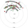 |
Fig. 1 Galactic position of the WN stars based on Gaia distances. The meaning of the different symbols is explained in the caption of Fig. 2. The labels refer to the WR catalog numbers. The Sun (⊙) and the Galactic Center (GC) are indicated. The WN stars trace the Galactic spiral arm structure as indicated schematically (after Vallée 2016) by the shaded arcs for the Perseus (outmost), Carina-Sagittarius (middle), and Crux-Centaurus (innermost) arm, respectively. |
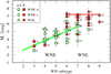 |
Fig. 2 Absolute narrow-band v-magnitudes of Galactic WN stars based on Gaia DR2 distances. The red symbols refer to stars with detectable hydrogen, while the green filled symbols stand for hydrogen-free stars. The symbol shapes refer to the spectral subtype: “early” and “late” subtypes (WNE and WNL, respectively) and distinguish among the WNE stars between weak (-w) and strong (-s) lines (see Paper I for details). The binaries and runaways are encircled (cf. Sect. 2). The labels refer to the WR catalog numbers; if printed with slanted font, their Gaia measurement is flagged with a significant astrometric excess noise (see Sect. 3). The thick lines indicate the subtype calibration adopted in Paper I. |
4 Rescaling of the stellar parameters
The spectroscopic parameters, which are not affected by the adopted distance, are repeated from Paper I in Cols. 3–8 of Table 1. One of these spectroscopic parameters is the transformed radius, i.e.,
![Mathematical equation: \begin{equation*}R_{\mathrm{t}} = R_{\ast} \left[ \frac{\varv_{\infty}}{2500\,\mathrm{km\,s^{-1}}} \left/ \frac{\dot{M} \sqrt{D} }{10^{-4}\, M_{\odot}\,\mathrm{yr^{-1}}} \right. \right]^{\frac{2}{3}} . \end{equation*}](/articles/aa/full_html/2019/05/aa34850-18/aa34850-18-eq2.png) (2)
(2)
In this equation, R* denotes the stellar radius that corresponds, by our definition, to a Rosseland continuum optical depth of τ = 20; Ṁ denotes the mass-loss rate; v∞ is the terminal wind velocity; and D is the clumping factor as introduced in Hamann & Koesterke (1998).
The (misleadingly termed) “transformed radius” has been defined (Schmutz et al. 1989; Hamann & Koesterke 1998) when realizing that normalized line spectra for WR stars of same T* depend only on Rt, but are nearly independent from the individual combination of the other parameters (especially, R* and Ṁ) that enter Eq. (2). Thus, the use of Rt reduces the dimension of the parameter space for which models must be provided; one can fit the normalized line spectrum with models for a “wrong” luminosity, and afterwards re-scale the spectral energy distribution according the observed flux (see Paper I for more explanations).
For a spherically extended object, the definition of an effective temperature depends on the reference radius. The stellar temperature T* (Col. 3) refers to the stellar radius R* defined above. Thus, the Stefan–Boltzmann equation
 (3)
(3)
relates R* and the corresponding (effective) stellar temperature T* to the stellar luminosity L.
By combining Eqs. (2) and (3) one can immediately obtain the corrections to the stellar luminosity, radius, and mass-loss rate that follow from a revision of the distance modulus by ΔDM:
![Mathematical equation: \begin{align}&\Delta\log L = 0.4 \cdot \Delta{\textrm{DM}},\\[2pt] &\Delta\log R_{\ast} = 0.2 \cdot \Delta{\textrm{DM}},\\[2pt] &\Delta\log\dot{M} = 0.3 \cdot \Delta{\textrm{DM}}. \vspace*{-2pt}\end{align}](/articles/aa/full_html/2019/05/aa34850-18/aa34850-18-eq4.png)
After being rescaled to the Gaia distances, the stellar parameters (R*, Ṁ, L) are compiled in Table 1, Cols. 11, 12, and 13, respectively. In Col. 14 we recalculate the “wind efficiency” η = Ṁv∞∕(L∕c), i.e., the ratio of the mechanical momentum of the wind to the radial momentum in the radiation field (per unit of time).
The last Col. 15 gives current stellar masses. These values are calculated from the mass-luminosity relation for helium-burning stars on the helium zero-age main sequence (ZAMS) taken from Gräfener et al. (2011). This approximation might actually not be adequate for all stars in our sample, especially not if hydrogen is still detected in their atmosphere. For all stars with XH > 0 and log L∕L⊙ > 5.5 we construct a special M − L relation for the WNL stage based on the evolutionary tracks for rotating single stars from Ekström et al. (2012) – see Fig. 7. The stellar mass as derived from that relation is given as second value in Col. 15. We note that the stellar masses are significantly larger only for very high luminosities (log L∕L⊙≳ 6.2) for which the tracks predict ongoing hydrogen burning in the core.
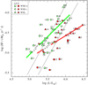 |
Fig. 3 Empirical mass-loss rate versus luminosity for the Galactic WN stars. Labels refer to the WR catalog numbers; if printed with slanted font, their Gaia measurement is flagged with a significant astrometric excess noise (see Sect. 3). The red symbols refer to stars with detectable hydrogen, while green symbols denote hydrogen-free stars (see inlet and caption of Fig. 2 for more details). Neither group follows a tight Ṁ − L relation. The thick green and red lines are linear regressions to the stars without and with hydrogen, respectively. The gray dotted lines denote the corresponding empirical relations from Nugis & Lamers (2000) for hydrogen-free WN stars (upper line) and for a hydrogen mass fraction of 40% (lower line). |
5 Results and discussion
5.1 Mass-loss rate versus luminosity
Radiation-driven mass loss is expected to depend, in first place, on the stellar luminosity. With the use of Gaia parallaxes, the stellar luminosities became more reliable. Therefore, we expected that the Ṁ − L−plot (Fig. 3) would show a better defined relation than obtained previously (cf. Paper I). However, the contrary is the case. The hydrogen-free stars (green symbols) show at least some correlation; the linear regression yields
 (7)
(7)
where the formal error of the slope is ± 0.18. The distribution of the red symbols (stars with hydrogen) looks even more messy. Obviously, this group of stars is by no means uniform; it contains stars in very different evolutionary stages and with quantitatively different hydrogen mass fraction in their winds. Formally, the linear regression to the red symbols yields
 (8)
(8)
where the formal error of the slope is ± 0.17.
The slopes of these regression lines are shallower than previously found. Figure 3 also shows the older empirical relations claimed by Nugis & Lamers (2000) that have a slope of 1.63 (gray dotted lines). However the shallow slopes found here resemble the value of 0.68 ± 0.05 obtained recently for the Galactic WC stars by Sander et al. (2019) using the new Gaia distances. Shallow slopes are in line with theoretical expectations from hydrodynamical models especially for the hydrogen-free stars because of their close proximity to the Eddington limit and the physics of wind-driving (Gräfener & Hamann 2008; Gräfener et al. 2011). For optically thick winds, Gräfener et al. (2017) predicted a slope of 1.3.
However, the empirical correlations shown in Fig. 3 are by no means tight, but have a large scatter. One might speculate that further parameters play a role, for example, different iron abundance or variations of the clumping properties. Since such parameters are not yet at hand, we refrain from a further discussion of the Ṁ dependencies. Closer studies of these questions would be interesting.
5.2 Hertzsprung–Russell diagram
The empirical HRD of our Galactic WN sample is shown in Fig. 4. As in the corresponding HRD in Paper I, the locations of the hydrogen-containing WNL stars and of the hydrogen-free WNE stars are found to be divided by the hydrogen ZAMS. Only a few WNL and WNE stars with hydrogen (red symbols in Fig. 4) violate this general rule. However, now using the Gaia distances, the WNL and WNE stars are not separated by a gap in luminosities anymore. Instead, in the range between log L∕L⊙ = 5.7 and 6.1 both subclasses can be found. This is in line with the population synthesis presented in Paper I.
We must remark on those symbols in the HRD that bear a little arrow to the left. As discussed in Paper I, there are a few stars in the sample that have such a thick wind that the entire spectrum is formed far out in the wind. In other words, the pseudo-photosphere expands with a significant fraction of the terminal velocity, while any quasi-static layers are deeply embedded and cannot be observed. Having adopted a β-law for the velocity field (cf. Paper I) throughout the supersonic part of the wind, we implicitly assume a steep velocity gradient for the inner wind region, and thus a stellar radius R* that is only slightly smaller than the radius from where the radiation emerges. However, if the velocity law in the lower, unobservable part of the wind would be in fact shallow, or if there was any other form of an “inflated envelope”, the quasi-static stellar “core” might have a significantly smaller radius than the pseudo-photosphere, thus potentially implying a much higher “stellar temperature” than the T* obtained by our analysis (cf. Eq. (3)). For such a thick atmosphere, the normalized line spectrum depends to first order only on the ratio L∕Ṁ4∕3, but not on T* and R*.
It is interesting to compare our empirical HRD for the Galactic WN stars with the corresponding HRD for single WN stars in the Large Magellanic Cloud (LMC), which had been analyzed in a similar way by Hainich et al. (2014) while distance uncertainties are not an issue for LMC members. Differences between the Galactic and the LMC sample can, in principle, have two reasons: the different metalicities, and a different star formation history.
Figure 5 reveals that the distributions of both samples are generally similar, but differ in detail. The LMC contains a few very luminous stars (BAT99 106, 108 and 109, Crowther et al. 2010) These stars all reside in the very active 30 Dor Starburst complex. Similarly, the most luminous members of our Galactic sample are preferably found in the Carina nebula, and thus also in a massive star-forming region. Obviously, such an environment is favorable for finding very massive stars.
The luminosity distribution of the LMC sample shows a pronounced gap between the seven most luminous stars and the numerous rest. A similar luminosity gap between the WNL and the WNE stars was originally visible in Paper I for the Galaxy as well, but is now filled with WNE and WNL stars as the result of the Gaia distances. Thus the bimodal distribution of WN luminosities found in Paper I was an artifact introduced by the subtype calibration of absolute magnitudes, but in the LMC it is real and probably reflects a particular age distribution.
At the lower end of the luminosity distribution, we find a couple of Galactic WNE stars, but no LMC counterparts. This can be explained in terms of single-star evolution by the metallicity dependence of stellar wind mass loss. Because of the lower metallicity in the LMC, the minimum mass required to bring an evolutionary track back to the hot side of the HRD is somewhat higher in the LMC than in the Galaxy (e.g., Meynet & Maeder 2005). If the WNE stars have lost their hydrogen envelope by Roche-lobe overflow (RLOF) in close-binary evolution, a metallicity dependence is not expected, and the observed difference between those two samples would have no obvious explanation.
Regarding the temperature distribution, the WN stars in the LMC appear to be slightly hotter than their Galactic counterparts; there are a few WNE stars residing even to the left of the helium ZAMS, and many WN stars with hydrogen are hotter than the hydrogen ZAMS. This could again indicate a metallicity effect. Since the LMC stars have slightly more compact cores and less thick winds, their spectra show higher stellar temperatures.
In Fig. 6 we compare the HRD positions of the Galactic WN sample studied in this paper with those of the Galactic WC and WO stars (Sander et al. 2019), which have also been updated according to the Gaia DR2 distances. The WC and WO stars must have evolved from hydrogen-free WN stars, when the latter have lost their helium layers and display the products of helium burning in their atmosphere. As Fig. 6 shows, the WC stars populate a similar range in luminosities as the WN stars with a slight tendency toward lower values, which is expected due to the progressing loss of mass. However, many WC stars have lower stellar temperatures than the WNE stars. Obviously, the evolution WNE → WC does not proceed toward higher T*. We conclude that the outer layers of a star become more “inflated” (Gräfener et al. 2012) at the transition from the WNE to the WC stage.
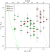 |
Fig. 4 Hertzsprung–Russell diagram of Galactic WN stars with Gaia parallax. The filling color reflects the surface composition (red: with hydrogen; green: hydrogen-free), while the symbol shape refers to the spectral subtype (see caption of Fig. 2). The binaries and runaways are encircled. The labels refer to the WR catalog numbers; if printed with slantedfont, their Gaia measurement is flagged with a significant astrometric excess noise (see Sect. 3). A little arrow indicates that for this particular star the indicated temperature is only a lower limit, because of the parameter degeneracy discussed in the text (Sect. 5.2). The vertical error bars reflect only the 1σ margin of the Gaia distances. Just for orientation, the ZAMS are indicated for solar composition and for pure helium stars, respectively. |
5.3 Stellar evolution
Various groups have published evolutionary tracks for massive stars with Galactic metallicity. A thorough comparison of our results with those various model predictions is beyond the scope of the present paper. In Fig. 7 we employ the Geneva tracks for Galactic metallicity (Z = 0.14) from Ekström et al. (2012), which account for rotationally induced mixing under the assumption that all stars rotate initially with 40% of their break-up rate.
At highest luminosities, the tracks (for initially 85 M⊙ and 120 M⊙) evolve from the hydrogen ZAMS immediately to the left, as expected for almost homogeneous stars, while the observed stars are in fact located slightly above or to the right of the ZAMS. It is not clear if this discrepancy could be attributed to envelope inflation. Such evolutionary models show core hydrogen burning and can in principle account for the more luminous members of the WNL stars observed.
The track for initially 60 M⊙ shows an unrealistic excursion to the red side, violating the Humphreys-Davidson limit. Apart from this, the lower half of the luminosity distribution of the hydrogen-displaying WNL stars can in principle be explained by tracks that return from the cool side, i.e., after having ignited core helium burning. Such tracks could then continue to the hotter, hydrogen-free WNE stars which now, with the revised distances, are found at similar luminosities. However, it seems to be a strange coincidence (and is not predicted in detail by the tracks) why the transition to hydrogen-free atmospheres should happen just when the track crosses a division line that apparently coincides with the hydrogen ZAMS. The location of the final WC/WO stage is in agreement with the observed locations of the Galactic WO stars WR 102 and WR 142 at 200 kK.
In the intermediate luminosity range, WN stars with and without hydrogen as well as WC stars are predicted by the tracks. The stellar temperatures are discrepant, which must be attributed to envelope inflation that is not reproduced by the evolutionary models. As already discussed above, especially the relatively cool temperatures of many WC stars imply that the evolution from the WNE to the WC stage is accompanied by a redward loop of the evolutionary track.
A significant number of WN stars in our sample and among the Galactic WC stars are found to have low luminosities that are not reproduced by the evolutionary tracks. The lowest mass for which the track reaches the WR stage is for initially 25 M⊙ (see Fig. 7), and even this star is predicted to explode before all hydrogen has been removed, i.e., it does not reach the hydrogen-free WNE and WC stages. The track for initially 20 M⊙ stays hydrogen-rich till the end. This could indicate that single-star evolution models still suffer from some deficiencies, possibly regarding the pre-WR mass-loss rates, rotational and other mixing processes, or core overshooting.
An alternative channel to produce WR stars invokes mass transfer in binary systems (Paczyński 1967). It has long been known that the majority of massive stars have been born in close binary systems (e.g., Vanbeveren et al. 1998).
If the primary star of a close binary falls in the suitable mass range (i.e., below 60 M⊙ according to the tracks in Fig. 7), it will expand when evolving until RLOF occurs. After its hydrogen envelope is removed (and partially accreted on the companion), the remaining star is expected to be hot and hydrogen depleted, thus retraining the spectral appearance of a WR star. Since this channel does not depend on wind mass loss, it can work at lower luminosities than the single-star evolution.
However, the secondary in this system would gain a lot of mass from RLOF, and thus would become most likely a bright and detectable OB star. For our sample stars, a currently present OB-type companion is observationally excluded (except for the few established binaries, see Sect. 2). Thus, such history cannot explain the apparently single WN stars of our sample.
As a theoretical possibility to avoid a bright companion, common envelope evolution has been proposed. If the secondary was originally a low-mass star (e.g., with 1 M⊙), it might have helped to eject the hydrogen envelope without accreting much mass itself (e.g., Kruckow et al. 2016), albeit there are energetic constraints to the possible parameters of such a scenario. Finally, the components might have merged. If it survived, such faint, low-mass companion might be very difficult to detect.
Alternatively, we may consider the possibility that the current WR star was originally the secondary of a binary system and served as the mass gainer in a first RLOF. Then the primary explodes or collapses to a compact object. If the system stayed bound after this event, a second RLOF phase could occur, this time from the original secondary to the compact object. This could help to strip off the hydrogen envelope from the secondary and turn it into a WR star. This channel would lead to a WR + compact companion system, which would be easily detected as a High Mass X-ray Binary, and therefore must also be ruled out for our sample – unless the compact companion is so deeply embedded in the WR wind that X-rays cannot emerge – as has been speculated recently for WR 124 (Toala et al. 2018). Even more exotic, the compact companion might have been engulfed in a merger process forming a kind of Thorne-Żytkow object, as has been occasionally speculated to be the nature of WN 8 stars (e.g., Foellmi & Moffat 2002).
Summarizing the discussion of the HRD, it seems that neither the single-star evolutionary models considered in this work, nor binary scenarios can provide a fully satisfactory explanation for the parameter distribution of the apparently single Galactic WN stars. Most likely, the single-star evolutionary calculations still suffer from incomplete physics, such as mass-loss recipes, internal mixing, and envelope inflation.
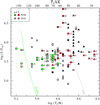 |
Fig. 5 Hertzsprung–Russell diagram of the WN stars in the LMC (adapted from Hainich et al. 2014). The filling color reflects the surface composition (red: with hydrogen; green: hydrogen-free), while the symbol shapes refer to the spectral subtype (see inlet). The labels refer to the BAT 99 catalog numbers (Breysacher et al. 1999). For comparison, the Galactic WN stars studied in the present paper are represented by the grey (hydrogen-free) and black symbols in the background. For orientation, the ZAMS are indicated for solar composition and for pure helium stars, respectively. |
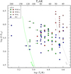 |
Fig. 6 Empirical HRD of the Galactic WN sample (green and red symbols, cf. Fig. 4), now additionally including Galactic WC and WO-type stars (blue symbols) from Sander et al. (2019). |
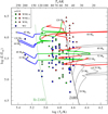 |
Fig. 7 Hertzsprung–Russell diagram of the Galactic Wolf-Rayet stars with Gaia distances (cf. Fig. 6) compared toevolutionary tracks for single stars from Ekström et al. (2012) which account for rotation. The tracks are colored analogously in the different WR stages, according to their predicted surface composition. The labels refer to the initial mass. |
6 Summary
Spectral analyses of a comprehensive set of Galactic WN stars, mostly putatively single, have been presented by Hamann et al. (2006; PaperI). These analyses were based on the comparison with synthetic spectra calculated with the Potsdam Wolf-Rayet (PoWR) non-LTE stellar atmosphere code.
- 1.
At the time of Paper I, the distances to the individual objects in this Galactic sample were poorly known. The distance uncertainty affects the “absolute” quantities derived from the spectral analysis, such as luminosity and mass-loss rate.
- 2.
Only recently, trigonometric parallaxes became available for the first time from the Gaia satellite (DR 2) for nearly all objects in this sample (now 55 objects). On average, the new distances are smaller by only 10% compared to the values adopted in Paper I. However, for some of the objects the revisions are substantial (−2.6 mag in distance modulus in the two most extreme cases).
- 3.
In this work, we keep the spectroscopic parameters from the analyses in Paper I, but rescale the results according to the new distances based on the Gaia parallaxes.
- 4.
The correlations between mass-loss rate and luminosity show a large scatter, for the hydrogen-free WN stars as well as for those with detectable hydrogen. The slopes of the log L − log Ṁ correlations are shallower than found previously.
- 5.
The empirical HRD still shows the previously established dichotomy between the hydrogen-free early WN subtypes, which are located on the hot side of the ZAMS, and the late WN subtypes, which show hydrogen and reside mostly at coolertemperatures than the ZAMS (with few exceptions).
- 6.
With the new distances, the distribution of stellar luminosities became more continuous than obtained previously. The hydrogen-showing WNL stars are still found to be typically more luminous than the hydrogen-free WNEs, but there is a range of luminosities (log L∕L⊙≈ 5.5 … 6.1) where both subclasses overlap.
- 7.
The empirical HRD of the Galactic single WN stars is compared with recent evolutionary tracks from Ekström et al. (2012). Neither these single-star evolutionary models nor binary scenarios can provide a fully satisfactory explanation for the parameters of these objects and their location in the HRD.
Acknowledgements
We thank the referee, P. Crowther, for his useful comments. This work has made use of data from the European Space Agency (ESA) mission Gaia (http://www.cosmos.esa.int/Gaia), processed by the Gaia Data Processing and Analysis Consortium (DPAC; http://www.cosmos.esa.int/web/gaia/dpac/consortium). Funding for the DPAC has been provided by national institutions, in particular the institutions participating in the Gaia Multilateral Agreement. R.H. was supported by the German Deutsche Forschungsgemeinschaft (DFG) project HA 1455/28-1. A.A.C.S. was supported by the DFG project HA 1455-26, and also thanks the STFC for funding under grant ST/R000565/1. T.S. acknowledges funding from the German “Verbundforschung” (DLR) grant 50 OR 1612 and from the European Research Council (ERC) under the European Union’s DLV_772225_MULTIPLES Horizon 2020 research and innovation programme. L.M.O acknowledges support from the DLR under grant 50 OR 1809 and partial support from the Russian Government Program of Competitive Growth of the Kazan Federal University.
References
- Abbott, D. C., Bieging, J. H., Churchwell, E., & Torres, A. V. 1986, ApJ, 303, 239 [NASA ADS] [CrossRef] [Google Scholar]
- Aldoretta, E. J., St-Louis, N., Richardson, N. D., et al. 2016, MNRAS, 460, 3407 [NASA ADS] [CrossRef] [Google Scholar]
- Arenou, F., Luri, X., Babusiaux, C., et al. 2018, A&A, 616, A17 [Google Scholar]
- Bailer-Jones, C. A. L., Rybizki, J., Fouesneau, M., Mantelet, G., & Andrae, R. 2018, AJ, 158, 58 [NASA ADS] [CrossRef] [Google Scholar]
- Breysacher, J., Azzopardi, M., & Testor, G. 1999, A&AS, 137, 117 [NASA ADS] [CrossRef] [EDP Sciences] [Google Scholar]
- Cardelli, J. A., Clayton, G. C., & Mathis, J. S. 1989, ApJ, 345, 245 [NASA ADS] [CrossRef] [Google Scholar]
- Chené, A. N., Foellmi, C., Marchenko, S. V., et al. 2011, A&A, 530, A151 [NASA ADS] [CrossRef] [EDP Sciences] [Google Scholar]
- Chené, A.-N., St-Louis, N., Moffat, A. F. J., et al. 2019, MNRAS, 484, 5834 [NASA ADS] [CrossRef] [Google Scholar]
- Churchwell, E., Bieging, J. H., van der Hucht, K. A., et al. 1992, ApJ, 393, 329 [NASA ADS] [CrossRef] [Google Scholar]
- Contreras, M. E., Rodriguez, L. F., Gomez, Y., & Velazquez, A. 1996, ApJ, 469, 329 [NASA ADS] [CrossRef] [Google Scholar]
- Crowther, P. A., Schnurr, O., Hirschi, R., et al. 2010, MNRAS, 408, 731 [NASA ADS] [CrossRef] [Google Scholar]
- Dorfi, E. A., Gautschy, A., & Saio, H. 2006, A&A, 453, L35 [NASA ADS] [CrossRef] [EDP Sciences] [Google Scholar]
- Ekström, S., Georgy, C., Eggenberger, P., et al. 2012, A&A, 537, A146 [NASA ADS] [CrossRef] [EDP Sciences] [Google Scholar]
- Fahed, R., & Moffat, A. F. J. 2012, MNRAS, 424, 1601 [NASA ADS] [CrossRef] [Google Scholar]
- Fitzpatrick, E. L. 1999, PASP, 111, 63 [NASA ADS] [CrossRef] [Google Scholar]
- Foellmi, C., & Moffat, A. F. J. 2002, in Stellar Collisions, Mergers and their Consequences, ed. M. M. Shara, ASP Conf. Ser., 263, 123 [NASA ADS] [Google Scholar]
- Gaia Collaboration (Prusti, T., et al.) 2016, A&A, 595, A1 [NASA ADS] [CrossRef] [EDP Sciences] [Google Scholar]
- Gamen, R., Goss, E., Morrell, N. I., et al. 2008, Rev. Mex. Astron. Astrofis. Conf. Ser., 33, 91 [NASA ADS] [Google Scholar]
- Gosset, E., Nazé, Y., Claeskens, J.-F., et al. 2005, A&A, 429, 685 [NASA ADS] [CrossRef] [EDP Sciences] [Google Scholar]
- Gräfener, G.,& Hamann, W.-R. 2008, A&A, 482, 945 [NASA ADS] [CrossRef] [EDP Sciences] [Google Scholar]
- Gräfener, G., Koesterke, L., & Hamann, W.-R. 2002, A&A, 387, 244 [NASA ADS] [CrossRef] [EDP Sciences] [Google Scholar]
- Gräfener, G., Vink, J. S., de Koter, A., & Langer, N. 2011, A&A, 535, A56 [NASA ADS] [CrossRef] [EDP Sciences] [Google Scholar]
- Gräfener, G., Owocki, S. P., & Vink, J. S. 2012, A&A, 538, A40 [NASA ADS] [CrossRef] [EDP Sciences] [Google Scholar]
- Gräfener, G., Owocki, S. P., Grassitelli, L., & Langer, N. 2017, A&A, 608, A34 [NASA ADS] [CrossRef] [EDP Sciences] [Google Scholar]
- Hainich, R., Rühling, U., Todt, H., et al. 2014, A&A, 565, A27 [NASA ADS] [CrossRef] [EDP Sciences] [Google Scholar]
- Hainich, R., Pasemann, D., Todt, H., et al. 2015, A&A, 581, A21 [Google Scholar]
- Hamann, W., & Koesterke, L. 1998, A&A, 335, 1003 [NASA ADS] [Google Scholar]
- Hamann, W.-R., & Gräfener, G. 2004, A&A, 427, 697 [NASA ADS] [CrossRef] [EDP Sciences] [Google Scholar]
- Hamann, W., Gräfener, G., & Liermann, A. 2006, A&A, 457, 1015 [NASA ADS] [CrossRef] [EDP Sciences] [Google Scholar]
- Kruckow, M. U., Tauris, T. M., Langer, N., et al. 2016, A&A, 596, A58 [NASA ADS] [CrossRef] [EDP Sciences] [Google Scholar]
- Lefèvre, L., Marchenko, S. V., Moffat, A. F. J., et al. 2005, ApJ, 634, L109 [NASA ADS] [CrossRef] [Google Scholar]
- Lindegren, L., Hernández, J., Bombrun, A., et al. 2018, A&A, 616, A2 [NASA ADS] [CrossRef] [EDP Sciences] [Google Scholar]
- Maeder, A. 2003, A&A, 399, 263 [NASA ADS] [CrossRef] [EDP Sciences] [Google Scholar]
- Marchant, P., Langer, N., Podsiadlowski, P., Tauris, T. M., & Moriya, T. J. 2016, A&A, 588, A50 [NASA ADS] [CrossRef] [EDP Sciences] [Google Scholar]
- Marchenko, S. V., Moffat, A. F. J., Lamontagne, R., & Tovmassian, G. H. 1996, ApJ, 461, 386 [NASA ADS] [CrossRef] [Google Scholar]
- Marchenko, S. V., Moffat, A. F. J., Eversberg, T., et al. 1998a, MNRAS, 294, 642 [NASA ADS] [CrossRef] [Google Scholar]
- Marchenko, S. V., Moffat, A. F. J., van der Hucht, K. A., et al. 1998b, A&A, 331, 1022 [NASA ADS] [Google Scholar]
- Meynet, G., & Maeder, A. 2005, A&A, 429, 581 [NASA ADS] [CrossRef] [EDP Sciences] [Google Scholar]
- Moffat, A. F. J., Lamontagne, R., & Seggewiss, W. 1982, A&A, 114, 135 [NASA ADS] [Google Scholar]
- Mokiem, M. R., de Koter, A., Vink, J. S., et al. 2007, A&A, 473, 603 [NASA ADS] [CrossRef] [EDP Sciences] [Google Scholar]
- Montes, G., Pérez-Torres, M. A., Alberdi, A., & González, R. F. 2009, ApJ, 705, 899 [NASA ADS] [CrossRef] [Google Scholar]
- Moran, J. P., Davis, R. J., Bode, M. F., et al. 1989, Nature, 340, 449 [NASA ADS] [CrossRef] [Google Scholar]
- Munoz, M., Moffat, A. F. J., Hill, G. M., et al. 2017, MNRAS, 467, 3105 [NASA ADS] [Google Scholar]
- Niemela, V. S., Shara, M. M., Wallace, D. J., Zurek, D. R., & Moffat, A. F. J. 1998, AJ, 115, 2047 [NASA ADS] [CrossRef] [Google Scholar]
- Nugis, T., & Lamers, H. J. G. L. M. 2000, A&A, 360, 227 [NASA ADS] [Google Scholar]
- Paczyński, B. 1967, Acta Astron., 17, 355 [NASA ADS] [Google Scholar]
- Paczynski, B. 1976, in Structure and Evolution of Close Binary Systems, eds. P. Eggleton, S. Mitton, & J. Whelan, IAU Symp., 73, 75 [Google Scholar]
- Pandey, J. C., Pandey, S. B., & Karmakar, S. 2014, ApJ, 788, 84 [NASA ADS] [CrossRef] [Google Scholar]
- Rauw, G., Vreux, J. M., Gosset, E., et al. 1996, A&A, 306, 771 [NASA ADS] [Google Scholar]
- Sana, H. 2017, in the Lives and Death-Throes of Massive Stars, eds. J. J. Eldridge, J. C. Bray, L. A. S. McClelland, & L. Xiao, IAU Symp., 329, 110 [Google Scholar]
- Sander, A., Todt, H., Hainich, R., & Hamann, W.-R. 2014, A&A, 563, A89 [NASA ADS] [CrossRef] [EDP Sciences] [Google Scholar]
- Sander, A. A. C., Hamann, W.-R., Todt, H., et al. 2019, A&A, 621, A92 [NASA ADS] [CrossRef] [EDP Sciences] [Google Scholar]
- Schmutz, W., Hamann, W., & Wessolowski, U. 1989, A&A, 210, 236 [NASA ADS] [Google Scholar]
- Seaton, M. J. 1979, MNRAS, 187, 73P [NASA ADS] [CrossRef] [Google Scholar]
- Shenar, T., Hainich, R., Todt, H., et al. 2016, A&A, 591, A22 [NASA ADS] [CrossRef] [EDP Sciences] [Google Scholar]
- Shenar, T., Richardson, N. D., Sablowski, D. P., et al. 2017, A&A, 598, A85 [NASA ADS] [CrossRef] [EDP Sciences] [Google Scholar]
- Shenar, T., Hainich, R., Todt, H., et al. 2018, A&A, 616, A103 [NASA ADS] [CrossRef] [EDP Sciences] [Google Scholar]
- Skinner, S. L., Itoh, M., Nagase, F., & Zhekov, S. A. 1999, ApJ, 524, 394 [NASA ADS] [CrossRef] [Google Scholar]
- Skinner, S. L., Zhekov, S. A., Güdel, M., Schmutz, W., & Sokal, K. R. 2012, AJ, 143, 116 [NASA ADS] [CrossRef] [Google Scholar]
- Smith, L. F. 1968, MNRAS, 140, 409 [NASA ADS] [Google Scholar]
- Smith, N., & Owocki, S. P. 2006, ApJ, 645, L45 [NASA ADS] [CrossRef] [Google Scholar]
- St-Louis, N. 2013, ApJ, 777, 9 [NASA ADS] [CrossRef] [Google Scholar]
- St-Louis, N., Tremblay, P., & Ignace, R. 2018, MNRAS, 474, 1886 [NASA ADS] [CrossRef] [Google Scholar]
- Tetzlaff, N., Neuhäuser, R., & Hohle, M. M. 2011, MNRAS, 410, 190 [NASA ADS] [CrossRef] [Google Scholar]
- Toala, J. A., Oskinova, L. M., Hamann, W.-R., et al. 2018, ApJ, 869, L11 [NASA ADS] [CrossRef] [Google Scholar]
- Vallée, J. P. 2016, AJ, 151, 55 [NASA ADS] [CrossRef] [Google Scholar]
- Vanbeveren, D., De Donder, E., van Bever, J., van Rensbergen, W., & De Loore C. 1998, New Astron., 3, 443 [NASA ADS] [CrossRef] [Google Scholar]
- Vanbeveren, D., Van Bever, J., & Belkus, H. 2007, ApJ, 662, L107 [NASA ADS] [CrossRef] [Google Scholar]
- Williams, P. M., Dougherty, S. M., Davis, R. J., et al. 1997, MNRAS, 289, 10 [NASA ADS] [Google Scholar]
- Zhekov, S. A., & Park, S. 2010, ApJ, 709, L119 [NASA ADS] [CrossRef] [Google Scholar]
All Tables
All Figures
|
Fig. 1 Galactic position of the WN stars based on Gaia distances. The meaning of the different symbols is explained in the caption of Fig. 2. The labels refer to the WR catalog numbers. The Sun (⊙) and the Galactic Center (GC) are indicated. The WN stars trace the Galactic spiral arm structure as indicated schematically (after Vallée 2016) by the shaded arcs for the Perseus (outmost), Carina-Sagittarius (middle), and Crux-Centaurus (innermost) arm, respectively. |
| In the text | |
|
Fig. 2 Absolute narrow-band v-magnitudes of Galactic WN stars based on Gaia DR2 distances. The red symbols refer to stars with detectable hydrogen, while the green filled symbols stand for hydrogen-free stars. The symbol shapes refer to the spectral subtype: “early” and “late” subtypes (WNE and WNL, respectively) and distinguish among the WNE stars between weak (-w) and strong (-s) lines (see Paper I for details). The binaries and runaways are encircled (cf. Sect. 2). The labels refer to the WR catalog numbers; if printed with slanted font, their Gaia measurement is flagged with a significant astrometric excess noise (see Sect. 3). The thick lines indicate the subtype calibration adopted in Paper I. |
| In the text | |
|
Fig. 3 Empirical mass-loss rate versus luminosity for the Galactic WN stars. Labels refer to the WR catalog numbers; if printed with slanted font, their Gaia measurement is flagged with a significant astrometric excess noise (see Sect. 3). The red symbols refer to stars with detectable hydrogen, while green symbols denote hydrogen-free stars (see inlet and caption of Fig. 2 for more details). Neither group follows a tight Ṁ − L relation. The thick green and red lines are linear regressions to the stars without and with hydrogen, respectively. The gray dotted lines denote the corresponding empirical relations from Nugis & Lamers (2000) for hydrogen-free WN stars (upper line) and for a hydrogen mass fraction of 40% (lower line). |
| In the text | |
|
Fig. 4 Hertzsprung–Russell diagram of Galactic WN stars with Gaia parallax. The filling color reflects the surface composition (red: with hydrogen; green: hydrogen-free), while the symbol shape refers to the spectral subtype (see caption of Fig. 2). The binaries and runaways are encircled. The labels refer to the WR catalog numbers; if printed with slantedfont, their Gaia measurement is flagged with a significant astrometric excess noise (see Sect. 3). A little arrow indicates that for this particular star the indicated temperature is only a lower limit, because of the parameter degeneracy discussed in the text (Sect. 5.2). The vertical error bars reflect only the 1σ margin of the Gaia distances. Just for orientation, the ZAMS are indicated for solar composition and for pure helium stars, respectively. |
| In the text | |
|
Fig. 5 Hertzsprung–Russell diagram of the WN stars in the LMC (adapted from Hainich et al. 2014). The filling color reflects the surface composition (red: with hydrogen; green: hydrogen-free), while the symbol shapes refer to the spectral subtype (see inlet). The labels refer to the BAT 99 catalog numbers (Breysacher et al. 1999). For comparison, the Galactic WN stars studied in the present paper are represented by the grey (hydrogen-free) and black symbols in the background. For orientation, the ZAMS are indicated for solar composition and for pure helium stars, respectively. |
| In the text | |
|
Fig. 6 Empirical HRD of the Galactic WN sample (green and red symbols, cf. Fig. 4), now additionally including Galactic WC and WO-type stars (blue symbols) from Sander et al. (2019). |
| In the text | |
|
Fig. 7 Hertzsprung–Russell diagram of the Galactic Wolf-Rayet stars with Gaia distances (cf. Fig. 6) compared toevolutionary tracks for single stars from Ekström et al. (2012) which account for rotation. The tracks are colored analogously in the different WR stages, according to their predicted surface composition. The labels refer to the initial mass. |
| In the text | |
Current usage metrics show cumulative count of Article Views (full-text article views including HTML views, PDF and ePub downloads, according to the available data) and Abstracts Views on Vision4Press platform.
Data correspond to usage on the plateform after 2015. The current usage metrics is available 48-96 hours after online publication and is updated daily on week days.
Initial download of the metrics may take a while.