| Issue |
A&A
Volume 624, April 2019
|
|
|---|---|---|
| Article Number | A43 | |
| Number of page(s) | 11 | |
| Section | Interstellar and circumstellar matter | |
| DOI | https://doi.org/10.1051/0004-6361/201833850 | |
| Published online | 05 April 2019 | |
Galactic H I supershells: kinetic energies and possible origin★
1
Instituto de Astronomía y Física del Espacio (CONICET-UBA), Ciudad Universitaria, C.A.B.A, Argentina
e-mail: This email address is being protected from spambots. You need JavaScript enabled to view it.
2
Instituto Argentino de Radioastronomía (CCT-La Plata, CONICET; CICPBA), C.C. No. 5, 1894 Villa Elisa, Argentina
3
Facultad de Ingeniería, Universidad de Buenos Aires (FIUBA), C.A.B.A, Argentina
4
Tensor Learning Unit - RIKEN Center for Advanced Intelligence Project, 1-4-1 Nihonbashi, Chuo-ku, 103-0027 Tokyo, Japan
5
Facultad de Ciencias Astronómicas y Geofísicas, Universidad Nacional de La Plata, La Plata, Argentina
Received:
13
July
2018
Accepted:
17
January
2019
Abstract
Context. The Milky Way, when viewed in the neutral hydrogen line emission, presents large structures called Galactic supershells (GSs). The origin of these structures is still a subject of debate. The most common scenario invoked is the combined action of strong winds from massive stars and their subsequent explosion as supernova.
Aims. The aim of this work is to determine the origin of 490 GSs that belong to the catalogue of H I supershell candidates in the outer part of the Galaxy.
Methods. To know the physical processes that took place to create these expanding structures, it is necessary to determine their kinetic energies. To obtain all the GS masses, we developed and used an automatic algorithm, which was tested on 95 GSs whose masses were also estimated by hand.
Results. The estimated kinetic energies of the GSs vary from 1 × 1047 to 3.4 × 1051 erg. Considering an efficiency of 20% for the conversion of mechanical stellar wind energy into the kinetic energy of the GSs, the estimated values of the GS energies could be reached by stellar OB associations. For the GSs located at high Galactic latitudes, the possible mechanism for their creation could be attributed to collision with high velocity clouds (HVC). We have also analysed the distribution of GSs in the Galaxy, showing that at low Galactic latitudes, |b| < 2°, most of the structures in the third Galactic quadrant seem to be projected onto the Perseus Arm. The detection of GSs at very high distances from the Galactic centre may be attributed to diffuse gas associated with the circumgalactic medium of M31 and to intra-group gas in the Local Group filament.
Key words: ISM: structure / methods: data analysis / techniques: image processing / radio lines: ISM
Tables 3 and 4 are only available at the CDS via anonymous ftp to cdsarc.u-strasbg.fr (130.79.128.5) or via http://cdsarc.u-strasbg.fr/viz-bin/qcat?J/A+A/624/A43
© ESO 2019
1 Introduction
The interstellar medium (ISM) of galaxies like the Milky Way has quite a complex structure where phases with different physical properties coexist. Immersed in this ISM are a plethora of features with a large variety of denominations like bubbles, shells, supershells, chimneys, worms, holes, and so forth, which have been observed to exist throughout the electromagnetic spectrum. Amongst the above features quite a few shells and their over-sized cousins, the supershells, are observable in the H I-line emission at a wavelength of 21 cm. Though there are in the astronomical literature a vast number of examples of H I-shells likely to be physically associated with massive stars and its descendants, and/or supernova remnants (e.g. Arnal 1992; Arnal et al. 1999, 2011; Cichowolski et al. 2001, 2009, 2014; Cappa et al. 2002, 2010; McClure-Griffiths et al. 2002; Cichowolski & Arnal 2004; Pineault et al. 2008; Reynoso et al. 2017), this is not the case for the majority of the catalogued Galactic supershells (GSs for short), where we considered GSs to those structures whose linear size is larger than 200 pc. Due to the physical association between H I shells and stars mentioned above, it is widely accepted that their genesis is likely to be deeply rooted in the interaction of the associated star(s) with its surrounding ISM, through the individual effects of their stellar winds or the combined action of stellar winds and the posterior supernova (SN) explosion of the massive stars. Since in most of the GSs the stellar counterpart possibly associated with them has not been observed, a stellar origin for the GSs similar to the one put forward for the H I-shells is far from being clear.
Furthermore, since for a few GSs their kinetic energy ( ) derived from the observations is very high, greater than 1052 ergs (Heiles 1979), it is thus unlikely to be provided by the combined action of stellar winds and SN explosions, unless we are willing to accept the existence in the past of stellar aggregates, open clusters, and/or OB associations that have an upper mass end much more populated than similar objects known to exist today in the Milky Way. For these extreme cases other plausible alternatives, like events connected to a gamma-ray burst (Perna & Raymond 2000) or the in-fall of high velocity clouds (HVC) into the Galactic H I disc (Tenorio-Tagle 1981), may be at work to create these large structures.
Knowledge of the kinetic energy of a sizable sample of GSs in our Galaxy may be a possible way to shed some light on the genesis of GSs. A “stellar option” for the genesis of GSs would be favorable if most of the GS’s mechanical energy is within the range that could be injected by the winds and SN explosions of the most massive members of the stellar aggregates, open clusters, and/or OB associations. Otherwise alternative options like those previously mentioned ought to be further explored. Though at first glance to derive the kinetic energy of a GS may appear rather simple, only the GS’s total mass and its expansion velocity are needed, the derivation of the mass is far from being trivial. Different researchers may apply different criteria for its derivation, resulting in mass estimates for the same object that may be quite different. Since the goal of this work is to determine in a systematic way the mechanical energy of a statistically significant sample of GSs, to this end a computer algorithm that automatically computes the GS masses was developed by one of us (CFC). This algorithm was applied to most of the objects catalogued as a GS by Suad et al. (2014). Though this catalogue contains a total of 566 structures, the algorithm was applied only to those GSs showing H I-emission surrounding its central cavity in at least three quarters (or 270°) of its angular extent. A total of 490 GSs fulfilled this criterion.
2 Observations
H I data were retrieved form the Leiden–Argentine–Bonn (LAB) survey (Kalberla et al. 2005). This database has an angular resolution of 34′, a velocity resolution of 1.3 km s−1, a channel separation of 1.03 km s−1, and it covers the velocity range from − 400 to + 450 km s−1. The entire database has been corrected for stray radiation (Kalberla et al. 2005).
3 Estimation of GS masses
As mentioned above, the GSs are large voids surrounded completely or partially by walls of H I emission. An example of such a structure, GS 153+02-047, listed in the catalogue of Suad et al. (2014), is shown in Fig. 1a, along with a profile of temperatures measured along a scan that crosses the central minimum as shown in Fig. 1b-top. Based on the hypothesis that before the structure was formed the H I was uniformly distributed, we can assume that the excess mass, or temperature, in the shell should be equal to the mass missing in the void. In Fig. 1b-bottom, the excess mass (shell mass, green) and missing mass (blue) are displayed for this particular example. Thus, we can estimate both the excess mass of the H I shell surrounding the cavity, denoted by  , and the mass missing in the void, which we shall refer to as the missing mass,
  . In an ideal case these two values should be exactly the same, however, owing to inhomogeneities present in the ISM where the structures are located, the estimated values for both masses do not always match.
Calculation of the H I masses is straightforward, first column densities are simply computed by integration of the difference in the mean brightness temperature( ) over the velocity range where the supershell is detected using
 (1)
(1)
under the assumption that the H I gas is optically thin. Then, the neutral mass of an H I structure of area A is given by
 (2)
(2)
For a structure located at a distance d and with an angular size Ω, A = Ω d2, and the mass can be easily estimated by
 (3)
(3)
which gives an approximation to an exact integral over velocity. We just take  as the velocity interval over which the GS is visible. In this equation, Ω is expressed in arcmin2 units.
3.1 Estimation by hand
In this section, we describe the procedure used to estimate the H I mass related to a structure by using Eq. (3) and the visualization and manipulation data program: Astronomical Image Processing System (AIPS). The first step is to determine all the involved parameters for the objects under consideration: distance, velocity interval where the structure is observed, angular size of the feature, and the mean temperature brightness difference ( ).
).
The distances of all the catalogued structures are given in Suad et al. (2014). The velocity interval where the supershell is better observed is determined by inspecting the H I data-cube, and is used to create a velocity averaged image. This averaged image is used to estimate the angular areas of the cavity (Ωcav) and the shell (Ωshell), and their corresponding averaged temperatures,  and
and  . Since
  and
and  are the excess mass in the shell and the missing mass in the cavity with respect to what it was in the region before the structure was formed, we define Tbg as the background temperature, that is the temperature that the uniform ISM had before the mass was swept-up in a shell structure (see Fig. 1b-top). Then, using Eq. (3), we estimate the shell masses by replacing
  by (
by ( ) and Ω by Ωshell; and the missing masses using
  = (
= ( ) and Ω = Ωcav.
Though the background temperature can be estimated considering the temperature of the H I emission located beyond the outer border of the GS, its determination is not straightforward. This stems from the fact that in most cases Tbg changes its value as we “move” around the outer part of the structure, due to variations that are intrinsic to the overall H I emission of the Milky Way. To determine it, we made several cuts in different directions of the structure and, from these profiles, we analysed what is the temperature of the gas emission not related to the structure.
All the estimated values have large uncertainties that must be taken into account in the value of the mass. For instance, given the non-uniform background, the determination of both the shell outer limit and the background temperature is usually quite subjective and not easy. To get an idea of the uncertainty involved in this measurement, the mass of each structure has been estimated by two of the authors of this work (Suad and Cichowolski). Comparing the obtained values we have concluded that on average the difference is of the order of 50%, both sides.
As another check of the accuracy of the estimated masses, we computed the background temperature local to each GS by forcing the missing and shell masses to be equal. The ratio between the temperature obtained in this way,  , and the one obtained by inspecting each structure, Tbg, is in the range between 1 and 1.2, indicating that the Tbg values used to compute the masses are in agreement with the hypothesis of
  and
and  being equal.
3.2 Algorithm for computing GS masses
In order to have a more precise estimation of the GS masses for a total of 490 structures included in the catalogue, we developed a computer-based algorithm and validated the results by comparing them against the values obtained “by hand” for a reduced subset of structures (see Sect. 4).
The algorithm has three parameters that need to be tuned (see Sect. 3.2.2). Two of them are structure-dependent parameters: the local maxima prune parameter α, and the outer wall extent parameter β; and one global parameter (for all shells in the catalogue): the maximum shell width parameter ΔR. The parameters are precisely defined in the algorithm description below.
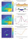 |
Fig. 1 Estimating the mass associated with a Galactic supershell, the example of GS 153+02-047: (a) averaged temperature image computed using the 70% of channels where the GS is detected in order to avoid the caps; (b) Top panel: temperature profile computed along the red line trajectory shown in a. The background temperature profile (black) is defined by connecting with a line the external limits of the shell. The averaged temperatures of the shell and the cavity are Tshell and Tcav, respectively. Bottom panel: temperature of the shell (green) is computed as the excess of temperature with respect to the background temperature level. The temperature associated with the missing mass (blue) is computed as the required temperature to be added in the cavity in order to reach the background level; (c) description of the algorithm for computing masses. Radial trajectories (red lines) are used for computing temperature profiles and detecting local maxima (black dots) and outer walls of the structure. Once local maxima are detected, the algorithm fits an ellipse to those points (black line); (d) details of the temperature profile computed based on the radial trajectory displayed in panel c; (e) image of the temperature of the shell as computed by subtracting the background from the measured temperature as explained in panel b and Eq. (6); (f) the global parameter ΔR is tuned such that the error of the algorithm (rmse) is minimized when it is compared against a subset of structures analysed “by hand”. The optimal value of this parameter is ΔR = 0.4. |
3.2.1 Algorithm description
For each of the structures in the catalogue, the algorithm performs the following steps:
– STEP 1 (Averaging). The average map of temperatures, Tb, is obtained by averaging 70% of the central channels in which the shell is detected. This simple technique allows us to use a single averaged image to estimate the mass of the shell. This choice of the percentage of considered channels allowed us to successfully remove the “caps” of the structure making the minimum visible in the average. Figure 1a shows the averaged image obtained for the structure GS 152+02−047.
– STEP 2 (Local maxima finding)
I. By setting the local minimum as the centre of the structure, the algorithm computes the temperature profiles T(r, θ) for 100 radial lines (trajectories) starting at the local minimum and moving outward, where r is the angular distance from the centre and θ is the angle of the radial trajectory (red line in Fig. 1c). For each of these profiles, the algorithm finds the peak temperature(local maximum) following the same criterion as used in the detection of the supershell candidates in Suad et al. (2014). More specifically, in order to avoid non-realistic local maxima due, for example, to noise, we use the following criteria: first, we admit local maxima to exist only beyond a point of minimum slope. In other words, we compute the slope of the temperatureprofile and search for the local maximum only for distances beyond a point where a minimum slope threshold of Tslp = 0.2K px−1 is exceeded. Second, a local maximum is defined in such a way that its brightness temperature exceeds by at least a threshold δT the brightness temperature of its surroundings. The value of δT = 0.4K was determined during the “learning phase” in our previous work Suad et al. (2014). Third, we only accept a local maximum if its temperatureexceeds the temperature at the minimum (centre of the shell) by a certain threshold. The value of this threshold depends on the position within the H I data cube. In Suad et al. (2014), we developed an interpolation technique to estimate an optimal threshold for every location in the data cube. Finally, the maximum temperature is denoted by Tmax = T(rM, θ), where rM is the distance from the minimum at which the maximum is attained. Figure 1d shows a particular temperature profile corresponding to the angle θ as shown in Fig. 1c.
II. An ellipse is fitted to the local maxima points and the effective radii is defined as  , where a and b are the semi-major and semi-minor axes of the fitted ellipse, respectively. Figure 1c shows the detected local maxima (black points) for a particular structure in the catalogue together with the fitted elipse (black line).
III. To avoid spurious local maxima, we filter out detected local maxima that are too far from the centre in relation to the rest of the points. Basically, we enforce the local maxima points to satisfy the constraint
 (4)
(4)
where α is the local maxima prune parameter to be determined and a is the semi-major axis of the fitted ellipse. Once the points that do not meet the criterion in Eq. (4) are removed, the algorithm repeats step II–III until convergence is reached.
– STEP 3 (Outer wall determination). For each radial profile we need to determine the background temperature (solid black line in Fig. 1b). To do so, we need to find the outer wall of the structure. The adopted criterion is to detect the point where the temperature drops by a factor β Tmax. Formally we define r* such that T(r*) = β Tmax, where β is the outer wall extent parameter to be estimated (see below) and Tmax is the maximum temperature. Additionally, we impose the outer walls to be at a distance lower than a percentage ΔR of the effective radii computed in a previous step. Summarizing, we define the position rout of the outer wall such that
 (5)
(5)
In Fig. 1c the final shape of the outer wall is shown (white line). It is worth noting that, sometimes, for some ranges in the angle θ local maxima are not available and the algorithm finds the outer wall by interpolating the wall found for the nearest local maxima.
– STEP 4 (Shell mass and missing mass estimation). Finally, for each of the radial lines (each θ ∈ (0, π)) where the temperature profiles were computed, we determine the background temperature Tbg (θ, r), with r ∈ (−rout(−θ), +rout(θ)) by connecting the outer wall points in both ends of the profile as shown in Fig. 1b (black line). Then, we obtain the temperature of the shell Tshell(θ, r) and the “missing” temperature Tmiss(θ, r) in every location (θ, r) of the shell as follows:

where the location (θ, r) in the right hand of the equations is avoided to simplify the notation, and h(x) is the Heaviside step function, that is, h(x) = x if x ≥ 0 and h(x) = 0 otherwise. It is noted that by combining the Tbg(θ, r) for all θ and r in the shell, we finally obtained a surface of background temperatures, which allowed us to compute Tshell(θ, r) and Tmiss(θ, r) in the shell. In Fig. 1e, the resulting image for the temperature associated with the shell, Tshell, is displayed. Finally, the total temperature of the shell and the missing temperature are computed by integrating these temperature images in the plane l − b and the associated shell and missing masses are computed through Eq. (3).
3.2.2 Parameter tuning
To tune the parameters α, β, and ΔR we used a grid-search approach by running the algorithm for a wide range of parameter values (α ∈ [0.2, 1.0], β ∈ [0, 0.75], and ΔR ∈ [0.1, 0.9]), computing the corresponding missing and shell masses for each case and choosing the optimal values according to the following criteria:
– Optimal choice of structure-dependent parameters α and β given ΔR. We choose the value of α to be more in a way that the area covered by the wall is as close as possible to the area of the fitted ellipse, which was already estimated for each shell in the catalogue in Suad et al. (2014). On the other side, the parameter β is tuned by minimizing the absolute difference between the Tshell and Tmiss for a given ΔR. We observed that the optimal value for these two parameters is different for each shell so we tune this parameter individually.
– Optimal choice of global parameter ΔR (maximum shell width). Once parameters α and β are tuned for each shell and each value of ΔR in a range, we choose the optimal ΔR as the one that minimizes the error in the estimation of the masses compared to the values obtained by hand, for a subset of 61 structures (Group A, see Sect. 4). To measure the global error estimating the masses of this subset of structures, we computed the root mean squared error (rmse), which is defined as
 (8)
(8)
where Mhand(n) and Malg(n) are the masses estimated by “hand” and by the algorithm for shell n, respectively.Figure 1e shows the obtained rmse as a function of ΔR. It is noted that the minimum rmse is obtained for ΔR = 0.4 for which the obtainedrmse is equal to 3.8 × 10⁴ M⊙.
We would like to point out that the normalized error measure, given by
was also estimated, but we noted that the impact on the results is mild. In this case we obtain an optimal ΔR = 0.3 instead of ΔR = 0.4. We decided, however, to consider ΔR = 0.4 because it is the one that best reproduces the mass values estimated by hand in the sense that the effectivenumber of coincidences between the masses obtained by the algorithm and by hand is higher.
4 Validation of the algorithm
Since the goal of this paper is to determine the kinetic energy stored in all the Galactic supershell candidates that have four or three filled quadrants in the recently published catalogue of Suad et al. (2014), we need first to be confident that the masses obtained by the algorithm are reliable. To test the values yielded by the algorithm, we have measured individually the masses of 95 GSs belonging to the catalogue, 61 of them with four filled quadrants (Group A from hereon) and the remaining 34 with three filled quadrants (Group B from hereon). It is important to mention that all 95 GSs were randomly selected.
Following the procedures described in Sects. 3.1 and 3.2 and using Eq. (3), we estimated the 95 GS masses by hand ( ; Hand) and by the algorithm (
 ; Alg.) for structures of Group A and B. They are listed in Tables 1 and 2. The distance d, and the velocity interval,
  , where each GS is visible were taken from the catalogue presented in Suad et al. (2014). Figure 2 shows a comparison between the shell masses,
  , obtained by hand and by the algorithm, for Group A and Group B. Assuming an error of 50% for all the estimations, the values obtained from both procedures agree in 93% (Group A) and 91% (Group B) of the structures.
To analyse the reasons for which the algorithm does not work correctly for some GSs, we have inspected in detail those GSs that show mass discrepancies. We found that for three (GS 2, 10, and 18; see Table 1) and two (GS 9 and 16; see Table 2) GSs belonging to Groups A and B, respectively, the problem arises from the fact that the algorithm detects emission in the interior cavity of the shell. This could be attributed to emission originated by gas not related to the GS, that is, background or foreground emission. As a consequence, the algorithm “sees” a smaller structure and yields a lower mass estimate. Another detected problem, found for GS 6 (see Table 1) and GS 34 (see Table 2), was that the algorithm fails in detecting the maxima defining the GSs because the H I emission associated with the GS is weak and does not differ from the background emission.
5 Results
Given that, as shown in Sect. 4, the algorithm works correctly in more than 90% of the structures used to test it, we can now use it to estimate the masses of the 490 GS candidates belonging to the Suad et al. (2014) catalogue. Among them, 308 are completely surrounded by walls of H I emission (Group A) and in the remaining 182 the central H I minimum is surrounded by ridges of H I emission in at least 270° of its angular extent (Group B).
Adopting solar abundances, the total gaseous mass of each GS is given by
 (9)
(9)
then, GS kinetic energies can be derived from
 (10)
(10)
where vexp is the GS expansion velocity and is taken to be equal to half the velocity interval where the structure is observed. The results are shown in Tables 3 and 4 for Groups A and B, respectively. The estimated errors are about 50% for the GS masses and 64% for the kinetic energies. It is important to mention that although the expansion velocity of an H I expanding structure is usually estimated as half the velocity interval where the structure is detected, this value is an upper limit of the actual expansion velocity, since the differential rotation of the Galaxy should be considered, especially for large structures, as was done by McClure-Griffiths et al. (2006) and Ehlerová & Palouš (2018). In this work, since we are dealing with 490 structures and many of them are located at high Galactic latitudes or large distances, where the available rotation models of the Galaxy are probably not adequate, we estimate the energies without considering the velocity gradient of the Galaxy but with the caution of knowing that the actual energy values may be lower.
To check to what extent the effect of the differential rotation affects the energies obtained, we have estimated the energy values using the rotation model of Brand & Blitz (1993). As a result we found that if we call f the quotient between the new expansion speed value and the previous one  , considering the 490 structures, f has an average value of 0.75. As for the new values of the energies, we found that for 85% of them they agree, within errors, with the previous estimated values.
As can be seen in the histograms presented in Fig. 3, we find that the kinetic energies are between 2.5 × 1047 and 3.4 × 1051 erg for Group A, and between 1 × 1047 and 1.4 × 1051 erg for Group B. Although we found some structures that have very high energies, the mean values are 8 × 1049 and 6 × 1049 erg for Groups A and B, respectively. Moreover, we found that for Group A(B), 77% (79%) of the GSs have energies lower than 0.5 × 1050 erg, and 94% (95%) lower than 2 × 1050 erg. Figure 4 shows a plot of the kinetic energies stored in the GSs versus their effective radius (Reff), considering different Galactic plane heights (z). We find a slight tendency in the relationship between the size and energy, in the sense that the larger structures have higher energies, only for structures closer to the Galacticplane (left panels of Fig. 4). Most of the structures (72 and 64% for Groups A and B, respectively) are located at |z| < 1 kpc (see both left panels). The mean kinetic energy and effective radius for structures belonging to Group A and located at |z| ≤ 1 kpc are 0.5 × 1050 erg and 256 pc, respectively. For GSs located at |z| > 1 kpc the mean values of energy and effective radius are 1.5 × 1050 erg and 441 pc. Regarding Group B, the mean values are 0.5 × 1050 erg and 259 pc for |z| ≤ 1 kpc, and 0.8 × 1050 erg and 433 pc for |z| > 1 kpc.
Figure 5 shows a plot of the kinetic energy of the GSs versus their kinematic ages, for Groups A (left panel) and B (right panel), considering different Galactic latitude intervals (indicated by different colours). The kinematic ages were taken from the GS candidates catalogue (Suad et al. 2014), where they were obtained by using t (Myr) = Reff (pc)∕vexp (km s−1). Bearing in mind that the assumed expansion velocities are upper limits, the ages obtained are lower limit values (they are, on average, a factor of 1.4 larger if the  is considered). No clear dependence between kinetic energy and kinematic age is detected. Both groups have similar mean kinematic ages, 49 ± 12 Myr (Group A) and 53 ± 13 Myr (Group B). It is important to note, however, that these estimated ages decrease if we assume that the GSs were created by the action of stellar winds, in which case their dynamical ages are given by t (Myr) = 0.6 Reff (pc)∕vexp (km s−1) (Weaver et al. 1977).
Another important parameter that can be derived from the estimated GS masses is the ambient density (n0) of the ISM local to each structure. By uniformly distributing the excess mass in the shell over the cavity where the mass is missing, the ambient density into which a GS is evolving can be derived as
 (11)
(11)
where  is in solar masses and “vol” is the volume of the cavity in pc3, and was calculated assuming a spherical geometry. These estimates were done only for the 95 GSs whose masses were computed by the algorithm and by hand, because the volume of individual cavities is not easy to define using the algorithm. We obtain n0 values going from 0.03 to 2.5 cm−3.
Figure 6 shows the relation between n0 and the effective radius of the GSs. It can be seen that the largest structures seem to be located in regions with lower ambient densities. We found that for GSs with an effective radius higher than 250 pc, the averaged ambient density is 0.25 cm−3, while for the rest it goes up to0.72 cm−3.
On the other hand, to analyse the dependence of the estimated ambient densities with respect to the GS’s location in the Galaxy, in Fig. 7 we plot them in a graph of Galactic latitude versus Galactocentric distance (R), considering three ambient density intervals. Ambient density values lower than 0.2 cm−3, between 0.2 and 0.4 cm−3, and greater than0.4 cm−3 are represented with blue, red, and green dots, respectively.
From Fig. 7 it is clear that, as expected, ambient densities greater than 0.4 cm−3 are located mostly between ±10° Galactic latitude and not beyond 14 kpc from the Galactic centre. Lower densities are located in a wider range of Galactic latitudes and Galactocentric distances.
GS masses comparison for Group A.
GS masses comparison for Group B.
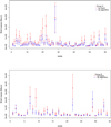 |
Fig. 2 Comparison between GS masses obtained by hand (red) and by the algorithm (blue) for Group A (top panel) and Group B (bottom panel). Vertical lines are shown considering a 50% error for every mass estimate. |
6 Discussion
As mentioned in Sect. 1, the action of massive stars is the most probable mechanism for the formation of shell structures. Taking into account the theoretical model of Weaver et al. (1977), the efficiency of conversion of mechanical stellar wind energy Ew into kinetic energy Ek is up to 20% for the energy conserving model. As was mentioned above, most of the structures has energies lower than 2 × 1050 erg, thus the wind energy needed to create a GS with this energy is Ew ~ 1 × 1051 erg. These values can be perfectly reached by stellar OB associations. For example an OB association with two O6.5, two O7, and three O8 V stars that contribute, during their main sequence (MS) phase, Ew ~ 1.1 × 1051 erg, could explain the origin of the GS. In the Galactic OB Associations in the Northern Milky Way Galaxy (Garmany & Stencel 1992), most of the OB associations fulfil this requirement. Open clusters, such as NGC 6193, are also capable of injecting the requiredwind energy.
Nevertheless, apart from the required energies, to analyse the origin of the GSs we have to take into account their ages. The fact that we found that most of the GSs are older than typical OB associations suggests that, for the formation of each structure, more than one generation of massive stars should be involved and that contributions from one or more supernova (SN) explosions are to be expected. Since, for example, the MS lifetime of an O7 type star is 6.4 Myr (Schaller et al. 1992), the earlier type stars, in an OB association, are expected to be evolved or have already exploded as a SN. Given that, assuming a stellar origin for the GS, only 19 are younger than 6.5 Myr, we do not expect to detect earlier type stars than an O7 V in the interior of most of them. On the other hand, taking into account that the SN rate in a typical OB association is about one per 105 –3 × 10⁵ yr (McCray & Kafatos 1987), over the lifetime of the GSs it is reasonable to assume that the most massive stars may have exploded.
For example, for one of the catalogued GSs, GS 100− 02−041, Suad et al. (2012) suggested that the wind energy provided during the main-sequence phase of the now evolved massive stars belonging to the OB association Cep OB1, and located inside GS 100−02−41, could explain the origin of the H I supershell, whose kinetic energy was estimated as 1.8 × 1050 erg. However, given the advanced age of the structure (5.5 Myr), they do not discard the possibility that a supernova explosion could have taken place.
Assuming that the genesis of the majority of the GSs was deeply rooted to the stellar winds and supernova explosions of massive stars, the location of the GS in the outer part of the Milky Way would suggest that in the past massive stars were located there.
The GSs’ spatial distribution in the outer part of the Milky Way is shown in Fig. 8, whilst the location of GSs, depending on their kinetic energy, is shown in Fig. 9. To plot the spiral arms of the Galaxy, we used the best-fitted models of polynomial-logarithmic (PL) spirals derived by Hou & Han (2014) using three kinds of spiral tracers (H II regions, giant molecular clouds, and masers). At first glance it is striking in both figures that a sizable fraction of the GSs present in the second Galactic quadrant are located at much larger Galactocentric distances than those located in the third quadrant. This finding was also pointed out by Ehlerová & Palouš (2013) in their analysis, where they also detected this asymmetry between the second and third Galactic quadrants in the distribution of shells at large Galactocentric distances. The origin of this observational result could be attributed to the gas distribution beyond the furthest spiral arm. Recent studies indicate that M31 has an extended gaseous halo (Lehner et al. 2015), suggesting that H I structures located at large distances could be formed in the circumgalactic medium of the Andromeda galaxy (M31) and in the intra-group gas in the Local Group filament, as was analysed in a recent paper by Richter et al. (2017).
On the other hand, as can be seen in Fig. 8, most of the GSs located at |b | ≤ 2° (upper panel) in the third Galactic quadrant seem to be projected onto the Perseus Arm and the Outer Arm. In this Galactic quadrant only a few GSs appear beyond the Outer Arm. At the extreme end of the Outer+1 Arm we can see a cumulus of several GSs. In the middle panel of Fig. 8, GSs located at 2° < |b| < 5° are plotted. As in the upper panel, there are several GSs delineating the Perseus and Outer Arms but, in this case, there are more GSs located beyond the Outer Arm. Beyond the Outer+1 Arm, GSs appear to be more dispersed than in the upper panel. Finally, in the bottom panel of Fig. 8 GSs located at |b | ≥ 5° are plotted. In the second Galactic quadrant there is an enhancement of GSs beyond the Outer Arm. Between 165° < l < 195° a lack of GSs is in evidence. This is because this region of the sky was not considered for Suad et al. (2014) to look for supershells, since the rotation curve used to derive kinematic distances is not trustworthy there.
We can conclude that GSs seem to be formed, at least for |b | ≤ 2°, in the Galactic spiral arms, which is consistent with a stellar origin. However, as shown in Fig. 8, there are some GSs located at higher Galactic latitudes, showing that if they also were formed by massive stars, these stars are or were present in this region of the Galaxy. As mentioned in Sect. 1, another possible origin for these GSs is collision with a HVC. As shown in Fig. 2 of Richter et al. (2017), there are a lot of HVC located at high latitudes, so it could be possible that some HVC played a role in the origin of some GSs.
The fact that we found GSs located at large Galactocentric distances, R > 15 kpc, may seem strange or inconsistent with a stellar origin since, until now, it was believed that massive stars were mostly located in the spiral arms. Nevertheless, a recent study of young star-forming regions associated with molecular clouds revealed that many of them are found at R ≥ 13.5 kpc, in the outer Galaxy (Izumi et al. 2017). They detected 711 new candidate star-forming regions in 240 molecular clouds. On the other hand, Anderson et al. (2015) detected H II regions located at Galactocentric distances greater than 19 kpc at l ~ 150°. Galactic H II regions are the formation sites of massive OB stars. These results strongly show that there is star formation activity in regions beyond the Outer and Outer+1 Arms. Concerning large H I structures, Cichowolski & Pineault (2011) detected a GS, GSH 91.5+2−114, in the outer part of the Galaxy, located at a distance of about 15 kpc from the Sun. Based on an analysis of the energetics and of the main physical parameters of the large shell, they conclude that GSH 91.5+2−114 is likely to be the result of the combined action of the stellar winds and supernova explosions of many stars.
Finally, Fig. 9 shows the location of the GSs with kinetic energies lower than 2 × 1050 ergs (Fig. 9a) and greater than 2 × 1050 erg (Fig. 9b). In Fig. 9a, the GSs appear more uniformly distributed in the second and third Galactic quadrants than in Fig. 9b, with a clear concentration towards the spiral arms. On the contrary, Fig. 9b shows that the most energetic structures are mostly located beyond the Outer and Outer+1 Arms.
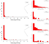 |
Fig. 3 Kinetic energy distributions for Group A and B in top and bottom panels, respectively. Right panels: energy distributions in more detail by showing structures with two energy ranges, lower–upper 1 × 1050 erg. |
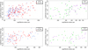 |
Fig. 4 Kinetic energy versus effective radius of the GSs for Group A (top panels) and B (bottom panels). Different coloured symbols represent different Galactic plane heights. Blue diamonds: |z| < 0.5 kpc, red squares: 0.5 < |z| < 1 kpc, green circles: 1 < |z| < 1.5 kpc, and violet triangles: |z| >1.5 kpc. |
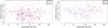 |
Fig. 5 Kinetic energies versus kinematic ages for GSs at different Galactic latitudes. Red points: GSs located at |b| ≤ 5°, blue triangles: GSs located at |b| > 5°. |
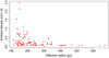 |
Fig. 6 Effective radius versus ambient density for the subsample of 95 GSs. |
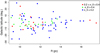 |
Fig. 7 Ambient density values distribution. Red dots represent ambient densities between 0.2 and 0.4 cm−3, green triangles and blue squares represent densities above 0.4 cm−3 and lower than 0.2 cm−3, respectively. |
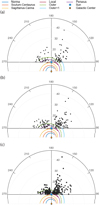 |
Fig. 8 Best-fitted models of polynomial-logarithmic (PL) spirals (Hou & Han 2014). Black points represent the GSs. Panel a: GSs located at |b | <= 2°. Panel b: GSslocated at 2° < |b| < 5°. Panel c: GSslocated at |b| >= 5°. The Sun is represented by a blue asterisk and the Galactic centre by a yellow dot. The concentric circles around the Galactic centre are separated by 10 kpc and indicate the distance to the Galactic centre. |
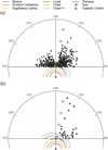 |
Fig. 9 Same Galactic model as in Fig. 8. Black points represent the GSs. In a and b panels, the GSs with Ek ≤ 2 × 1050 erg and Ek > 2 × 1050 erg, respectively, are plotted. |
7 Conclusions
In this paper, we have estimated the amount of H I mass of each supershell candidate belonging to the Suad et al. (2014) catalogue using an automatic algorithm, which was tested by a comparison of the results it gives with the ones obtain by hand, for 95 structures. For the analysis we divided the GSs into two groups: those with four filled quadrants belong to Group A and those with three filled quadrants to Group B.
The analysis of the obtained energies allows us to draw the following conclusions:
95% of the supershells have kinetic energies lower than 2 × 1050 erg, which, for a stellar origin, implies that a wind energy greater than 1 × 1051 erg is required.
There is no clear correlation between the energy stored in a shell and its kinematic age. With respect to the linear size, we find that the size increases accordingly as the energy increases only in those structures located near the Galactic plane.
Although there is no clear difference in the energy values found for Groups A and B, we found out that for |z| > 1 kpc, the mean kinetic energy for GSs belonging to Group A is larger than the one found for Group B. This may indicate that kinetic energy is being lost in the open structures.
According to the interval of energies obtained, a stellar origin is possible for most of the GSs. However, more than one star is needed and, in most of the cases, given that their ages are not extremely young, more than one stellar generation, including several SN explosions.
An origin due to a collision with a HVC is also possible, especially for those GSs located at very high latitudes.
The GSs found at very high distances from the Galactic centre may be formed by the diffuse gas that connects the stellar body of our Galaxy with the Local Group environment.
In summary, we conclude that most of the large H I structures found in the outer part of the Galaxy could have been created by the action of several generations of massive stars and SN
explosions. If this is actually the case, the GSs may be used to look for massive stars not yet detected and/or to better understand the massive stellar formation and distribution history.
Acknowledgements
This work was partially financed by grants PIP 0226 and PIP 0604 of the Consejo Nacional de Investigaciones Científicas y Técnicas (CONICET) of Argentina. We would like to thank the anonymous referee for constructive and useful comments that helped us to considerably improve the quality of the original paper.
References
- Anderson, L. D., Armentrout, W. P., Johnstone, B. M., et al. 2015, ApJS, 221, 26 [NASA ADS] [CrossRef] [Google Scholar]
- Arnal, E. M. 1992, A&A, 254, 305 [NASA ADS] [Google Scholar]
- Arnal, E. M., Cappa, C. E., Rizzo, J. R., & Cichowolski, S. 1999, AJ, 118, 1798 [NASA ADS] [CrossRef] [Google Scholar]
- Arnal, E. M., Cichowolski, S., Pineault, S., Testori, J. C., & Cappa, C. E. 2011, A&A, 532, A9 [NASA ADS] [CrossRef] [EDP Sciences] [Google Scholar]
- Brand, J., & Blitz, L. 1993, A&A, 275, 67 [NASA ADS] [Google Scholar]
- Cappa, C., Pineault, S., Arnal, E. M., & Cichowolski, S. 2002, A&A, 395, 955 [NASA ADS] [CrossRef] [EDP Sciences] [Google Scholar]
- Cappa, C. E., Vasquez, J., Pineault, S., & Cichowolski, S. 2010, MNRAS, 403, 387 [NASA ADS] [CrossRef] [Google Scholar]
- Cichowolski, S., & Arnal, E. M. 2004, A&A, 414, 203 [NASA ADS] [CrossRef] [EDP Sciences] [Google Scholar]
- Cichowolski, S., & Pineault, S. 2011, A&A, 525, A121 [NASA ADS] [CrossRef] [EDP Sciences] [Google Scholar]
- Cichowolski, S., Pineault, S., Arnal, E. M., et al. 2001, AJ, 122, 1938 [NASA ADS] [CrossRef] [Google Scholar]
- Cichowolski, S., Pineault, S., Gamen, R., et al. 2014, MNRAS, 438, 1089 [NASA ADS] [CrossRef] [Google Scholar]
- Cichowolski, S., Romero, G. A., Ortega, M. E., Cappa, C. E., & Vasquez, J. 2009, MNRAS, 394, 900 [NASA ADS] [CrossRef] [Google Scholar]
- Ehlerová, S., & Palouš, J. 2013, A&A, 550, A23 [NASA ADS] [CrossRef] [EDP Sciences] [Google Scholar]
- Ehlerová, S., & Palouš, J. 2018, A&A, 619, A101 [NASA ADS] [CrossRef] [EDP Sciences] [Google Scholar]
- Garmany, C. D., & Stencel, R. E. 1992, A&AS, 94, 211 [NASA ADS] [Google Scholar]
- Heiles, C. 1979, ApJ, 229, 533 [NASA ADS] [CrossRef] [Google Scholar]
- Hou, L. G., & Han, J. L. 2014, A&A, 569, A125 [NASA ADS] [CrossRef] [EDP Sciences] [Google Scholar]
- Izumi, N., Kobayashi, N., Yasui, C., Saito, M., & Hamano, S. 2017, AJ, 154, 163 [NASA ADS] [CrossRef] [Google Scholar]
- Kalberla, P. M. W., Burton, W. B., Hartmann, D., et al. 2005, A&A, 440, 775 [NASA ADS] [CrossRef] [EDP Sciences] [Google Scholar]
- Lehner, N., Howk, J. C., & Wakker, B. P. 2015, ApJ, 804, 79 [NASA ADS] [CrossRef] [Google Scholar]
- McClure-Griffiths, N. M., Dickey, J. M., Gaensler, B. M., & Green, A. J. 2002, ApJ, 578, 176 [NASA ADS] [CrossRef] [Google Scholar]
- McClure-Griffiths, N. M., Ford, A., Pisano, D. J., et al. 2006, ApJ, 638, 196 [NASA ADS] [CrossRef] [Google Scholar]
- McCray, R., & Kafatos, M. 1987, ApJ, 317, 190 [NASA ADS] [CrossRef] [Google Scholar]
- Perna, R., & Raymond, J. 2000, ApJ, 539, 706 [NASA ADS] [CrossRef] [Google Scholar]
- Pineault, S., Arnal, E. M., Cappa, C., et al. 2008, MNRAS, 386, 1739 [NASA ADS] [CrossRef] [Google Scholar]
- Reynoso, E. M., Cichowolski, S., & Walsh, A. J. 2017, MNRAS, 464, 3029 [NASA ADS] [CrossRef] [Google Scholar]
- Richter, P., Nuza, S. E., Fox, A. J., et al. 2017, A&A, 607, A48 [NASA ADS] [CrossRef] [EDP Sciences] [Google Scholar]
- Schaller, G., Schaerer, D., Meynet, G., & Maeder, A. 1992, A&AS, 96, 269 [Google Scholar]
- Suad, L. A., Cichowolski, S., Arnal, E. M., & Testori, J. C. 2012, A&A, 538, A60 [NASA ADS] [CrossRef] [EDP Sciences] [Google Scholar]
- Suad, L. A., Caiafa, C. F., Arnal, E. M., & Cichowolski, S. 2014, A&A, 564, A116 [NASA ADS] [CrossRef] [EDP Sciences] [Google Scholar]
- Tenorio-Tagle, G. 1981, A&A, 94, 338 [Google Scholar]
- Weaver, R., McCray, R., Castor, J., Shapiro, P., & Moore, R. 1977, ApJ, 218, 377 [NASA ADS] [CrossRef] [Google Scholar]
All Tables
All Figures
|
Fig. 1 Estimating the mass associated with a Galactic supershell, the example of GS 153+02-047: (a) averaged temperature image computed using the 70% of channels where the GS is detected in order to avoid the caps; (b) Top panel: temperature profile computed along the red line trajectory shown in a. The background temperature profile (black) is defined by connecting with a line the external limits of the shell. The averaged temperatures of the shell and the cavity are Tshell and Tcav, respectively. Bottom panel: temperature of the shell (green) is computed as the excess of temperature with respect to the background temperature level. The temperature associated with the missing mass (blue) is computed as the required temperature to be added in the cavity in order to reach the background level; (c) description of the algorithm for computing masses. Radial trajectories (red lines) are used for computing temperature profiles and detecting local maxima (black dots) and outer walls of the structure. Once local maxima are detected, the algorithm fits an ellipse to those points (black line); (d) details of the temperature profile computed based on the radial trajectory displayed in panel c; (e) image of the temperature of the shell as computed by subtracting the background from the measured temperature as explained in panel b and Eq. (6); (f) the global parameter ΔR is tuned such that the error of the algorithm (rmse) is minimized when it is compared against a subset of structures analysed “by hand”. The optimal value of this parameter is ΔR = 0.4. |
| In the text | |
|
Fig. 2 Comparison between GS masses obtained by hand (red) and by the algorithm (blue) for Group A (top panel) and Group B (bottom panel). Vertical lines are shown considering a 50% error for every mass estimate. |
| In the text | |
|
Fig. 3 Kinetic energy distributions for Group A and B in top and bottom panels, respectively. Right panels: energy distributions in more detail by showing structures with two energy ranges, lower–upper 1 × 1050 erg. |
| In the text | |
|
Fig. 4 Kinetic energy versus effective radius of the GSs for Group A (top panels) and B (bottom panels). Different coloured symbols represent different Galactic plane heights. Blue diamonds: |z| < 0.5 kpc, red squares: 0.5 < |z| < 1 kpc, green circles: 1 < |z| < 1.5 kpc, and violet triangles: |z| >1.5 kpc. |
| In the text | |
|
Fig. 5 Kinetic energies versus kinematic ages for GSs at different Galactic latitudes. Red points: GSs located at |b| ≤ 5°, blue triangles: GSs located at |b| > 5°. |
| In the text | |
|
Fig. 6 Effective radius versus ambient density for the subsample of 95 GSs. |
| In the text | |
|
Fig. 7 Ambient density values distribution. Red dots represent ambient densities between 0.2 and 0.4 cm−3, green triangles and blue squares represent densities above 0.4 cm−3 and lower than 0.2 cm−3, respectively. |
| In the text | |
|
Fig. 8 Best-fitted models of polynomial-logarithmic (PL) spirals (Hou & Han 2014). Black points represent the GSs. Panel a: GSs located at |b | <= 2°. Panel b: GSslocated at 2° < |b| < 5°. Panel c: GSslocated at |b| >= 5°. The Sun is represented by a blue asterisk and the Galactic centre by a yellow dot. The concentric circles around the Galactic centre are separated by 10 kpc and indicate the distance to the Galactic centre. |
| In the text | |
|
Fig. 9 Same Galactic model as in Fig. 8. Black points represent the GSs. In a and b panels, the GSs with Ek ≤ 2 × 1050 erg and Ek > 2 × 1050 erg, respectively, are plotted. |
| In the text | |
Current usage metrics show cumulative count of Article Views (full-text article views including HTML views, PDF and ePub downloads, according to the available data) and Abstracts Views on Vision4Press platform.
Data correspond to usage on the plateform after 2015. The current usage metrics is available 48-96 hours after online publication and is updated daily on week days.
Initial download of the metrics may take a while.