| Issue |
A&A
Volume 623, March 2019
|
|
|---|---|---|
| Article Number | A127 | |
| Number of page(s) | 8 | |
| Section | Catalogs and data | |
| DOI | https://doi.org/10.1051/0004-6361/201834591 | |
| Published online | 18 March 2019 | |
A homogeneous sample of 34 000 M7−M9.5 dwarfs brighter than J = 17.5 with accurate spectral types⋆
Astrophysics Group, Imperial College London, Blackett Laboratory, Prince Consort Road, London, SW7 2AZ, UK
e-mail: s.j.warren@imperial.ac.uk
Received:
6
November
2018
Accepted:
24
February
2019
The space density of late M dwarfs, subtypes M7–M9.5, is not well determined. We applied the photo-type method to iz photometry from the Sloan Digital Sky Survey and YJHK photometry from the UKIRT Infrared Deep Sky Survey, over an effective area of 3070 deg2, to produce a new, bright J(Vega) < 17.5, homogeneous sample of 33 665 M7–M9.5 dwarfs. The typical S/N of each source summed over the six bands is > 100. Classifications are provided to the nearest half spectral subtype. Through a comparison with the classifications in the BOSS Ultracool Dwarfs (BUD) spectroscopic sample, the typing is shown to be accurately calibrated to the BUD classifications and the precision is better than 0.5 subtypes rms; i.e. the photo-type classifications are as precise as good spectroscopic classifications. Sources with large χ2 > 20 include several catalogued late-type subdwarfs. The new sample of late M dwarfs is highly complete, but there is a bias in the classification of rare peculiar blue or red objects. For example, L subdwarfs are misclassified towards earlier types by approximately two spectral subtypes. We estimate that this bias affects only ∼1% of the sources. Therefore the sample is well suited to measure the luminosity function and investigate the softening towards the Galactic plane of the exponential variation of density with height.
Key words: stars: low-mass / catalogs / surveys
Full Table 1 is only available at the CDS via anonymous ftp to cdsarc.u-strasbg.fr (130.79.128.5) or via http://cdsarc.u-strasbg.fr/viz-bin/qcat?J/A+A/623/A127.
© ESO 2019
1. Introduction
A detailed census and study of the coolest stellar objects, i.e. late M dwarfs and cooler, first became possible with the implementation of wide-field surveys at wavelengths 0.8 − 2.4 μm, especially the Sloan Digital Sky Survey (SDSS; York et al. 2000) and the Two Micron All Sky Survey (2MASS; Skrutskie et al. 2006). The highlight in this area was the discovery and characterisation of the L and T dwarf populations (Kirkpatrick et al. 1999; Martín et al. 1999; Strauss et al. 1999; Geballe et al. 2002; Burgasser et al. 2002, 2006; Hawley et al. 2002; Schmidt et al. 2010). At the same time new insights into the properties of M dwarfs have been obtained, including the quantification of their activity as a function of spectral type and age (West et al. 2008, 2011; Schmidt et al. 2015), as well as measurement of the luminosity function (LF; Cruz et al. 2007; Covey et al. 2008; Bochanski et al. 2010). From the LF, using a relation between luminosity and mass (e.g. Delfosse et al. 2000), the stellar initial mass function (IMF) may be derived. The LF of M dwarfs is important because the characteristic mass of a log-normal fit to the IMF lies within this spectral range (Chabrier 2003; Bochanski et al. 2010).
The study by Bochanski et al. (2010) is the most complete analysis of the M dwarf LF. They determined new photometric parallax relations (absolute magnitude as a function of colour) and applied these values to a sample of ∼15 × 106 M dwarfs from 8400 deg2 of SDSS Data Release 7 to derive the LF over the absolute magnitude interval 7 < Mr(AB) < 16. Their LF varies smoothly over the interval 7 < Mr(AB) < 14, corresponding to spectral types M0–M5, but displays significant fluctuations between bins for absolute magnitudes Mr(AB) > 14. This is partly owing to the relatively small numbers at these absolute magnitudes, which is a consequence of their use of the r band for the sample magnitude limit, r(AB) = 22. Because late M dwarfs, > M5, are so red, imposing a cut in r leads to a rapid reduction in limiting distance, and thus sample size, towards later spectral types. The space densities for the latest M dwarfs are additionally uncertain because the photometric parallax relation is less well calibrated in this region. The measured IMF is further impacted because the colour correction from the r band to the J band, which is the passband of the Delfosse et al. (2000) mass-luminosity relation, is large for late M dwarfs and not precisely determined (Hawley et al. 2002).
An independent estimate of the M dwarf LF for spectral types M7–M9 was made by Cruz et al. (2007), using a sample of 53 stars within 20 pc of the Sun. The objects were identified using 2MASS JHKs photometry by application of a colour cut J − Ks > 1.0. Cruz et al. (2007) estimated that 79% of M7 dwarfs are redder than this colour limit and all M8 and M9 dwarfs. Unfortunately this sample is also problematic. Recent analysis of the 2MASS colours of M dwarfs by Schmidt et al. (2015) provided median colours J − Ks = 0.96, 1.03 for M7, M8. These results suggest that only ∼50% of M7 and M8 dwarfs satisfy the above colour cut, meaning their space densities have been substantially underestimated.
These questions motivate the compilation of a new sample of late M dwarfs, hereafter M7−M9.5, in order to obtain an improved measurement of the LF. We now briefly consider the issues involved in making an accurate measurement of the LF. Various studies of the LF may be distinguished by whether distances are measured by trigonometric, spectroscopic (absolute magnitude as a function of spectral type), or photometric parallax. The precision of the distances decreases along this sequence, but this is usually compensated by the increase in sample size. Trigonometric parallaxes can only be measured for the nearest, brightest sources, and similarly close binaries can only be resolved for the nearest sources. In comparison, for the largest samples that use photometric parallax, the distances are less precise and a statistical correction for unresolved binaries must be made. The variation in space density over the volume surveyed, because of the structure of the Milky Way, further complicates the measurement of the LF. These factors mean that comparison between local (such as Cruz et al. 2007) and distant (such as Bochanski et al. 2010) determinations of the LF is usually not straightforward. For reference, about one quarter of the Cruz et al. (2007) sources benefit from a trigonometric parallax, while the remainder have spectroscopic parallaxes.
In this paper we present a new large homogeneous sample of 34 000 M7−M9.5 dwarfs. We use “homogeneous” to mean that the sample has high completeness and for which the incompleteness is accurately quantified. The new sample exploits the deeper UKIRT Infrared Deep Sky Survey (UKIDSS) photometry (Lawrence et al. 2007), compared to 2MASS, and combines some of the respective advantages of the two previous studies, in that it is not only large but also benefits from precise distances. The sample approximates a complete spectroscopic sample: we use the phototype method of Skrzypek et al. (2015, 2016), combining SDSS iz and UKIDSS YJHK photometry, to measure accurate spectral types. The spectroscopic parallax relation of Dupuy & Liu (2012) then provides distances precise to 15%. All the M dwarfs in the new sample lie within 235 pc of the Sun. In a companion paper (Warren & Saad, in prep.) we will analyse the sample to measure the space density as a function of spectral type, which is equivalent to the LF.
The layout of the remainder of the paper is as follows. We describe the sample selection in Sect. 2. The sample and its main characteristics are presented in Sect. 3. In Sect. 4 we quantify the precision of the spectral typing. We summarise in Sect. 5.
2. Selection
2.1. Photo-type method
The photo-type method (Skrzypek et al. 2015) uses multiband photometry to measure spectral types. The wide wavelength coverage can compensate for the very low wavelength resolution of broadband photometry, and with high signal-to-noise ratio data photo-type classifications of late-type dwarfs are competitive with spectroscopic classifications in precision of spectral typing. Skrzypek et al. (2015) developed the method using SDSS+UKIDSS+ALLWISE izYJHKW1W2 8-band photometry for the discovery of L and T dwarfs in wide-field survey data. Using a set of stars and brown dwarfs classified by standard spectroscopic methods, polynomial relations between colour and spectral type were determined for the seven colours1. A source is then classified by fitting the spectral energy distribution (SED) against the set of templates for each MLT spectral subtype, as well as a range of templates for quasars and other possible contaminants, selecting the min-χ2 fit as the classification. The χ2 of the best fit is useful for identifying sources with spurious photometry and interesting peculiar objects.
In Skrzypek et al. (2016) the method was applied to the classification of point sources in the magnitude range 13.0 < J < 17.5, with colours Y − J > 0.8, resulting in a sample of 1281 L and 80 T dwarfs, from an effective area of 3070 deg2. The matching radius criteria (within UKIDSS, and in matching to SDSS and WISE) ensures that incompleteness due to proper motion is negligible. The effective area calculation accounts for sources lost due to unreliable photometry in any of the bands from a variety of causes. The relative depths in the different bands, the matching criteria, and the J magnitude range mean that incompleteness due to the requirement that a source is detected in all of the YJHK bands is negligible. The result is that the sample is essentially complete for all spectral types L0–T8, other than a small incompleteness that is estimated at 3% because peculiar blue L dwarfs are classified M and a related overcompleteness because peculiar red M dwarfs are classified L.
2.2. Selection of M7–M9.5 dwarfs
The goal of the current paper is to extend the survey of Skrzypek et al. (2016) to earlier spectral types M7–M9.5. The methods used are almost identical to those previously used. Small modifications to this approach mostly result from the difficulty to scrutinise all the images of all the objects in the much larger sample of over 30 000 late M dwarfs compared to 1361 L and T dwarfs. In this work we provide only a brief outline of the methods, deferring to the earlier papers for details, but we explain any differences in depth. Because we used almost identical procedures for the sample of late M dwarfs, we assume that the effective area calculated for the LT sample, 3070 deg2, also applies to the M dwarfs. We also assume that contamination of the sample by giants is negligibly small based on the arguments presented by Ferguson et al. (2017).
The photometric bands used in this study are the i and z bands in SDSS and the YJHK bands in UKIDSS. All the magnitudes and colours quoted in this paper are Vega based, unless explicitly labelled as AB, by for example r(AB). The YJHK survey data are calibrated to Vega, while SDSS is calibrated on the AB system. We applied the offsets tabulated in Hewett et al. (2006) to convert the SDSS iz AB magnitudes to Vega.
Starting with a set of point sources in the UKIDSS Large Area Survey data release 10, detected in all four bands, YJHK, and in the range 13.0 < J < 17.5, we matched to SDSS DR9 using a 10″ match radius and selected the point spread function (psf) photometric measurements. We note that a M7 dwarf has colours i − z = 1.36, Y − J = 0.68 (Skrzypek et al. 2016), and so we apply colour cuts i − z > 1.0, Y − J > 0.4 to reduce the total number of sources, while ensuring all sources M7 and later are retained (this assumption is checked later). To allow for sources with significant proper motion, we match to the nearest SDSS source that does not have a closer match to a different UKIDSS source. Considering the izYJHK colours of M7–M9.5 dwarfs (Skrzypek et al. 2016), and the limiting depths in the different bands, sources with 13.0 < J < 17.5 are easily detected in all the other bands. A small number of the faintest M7–M9.5 dwarfs do not have photometry in the ALLWISE W1 and W2 bands because the sources are undetected in both bands; a source only needs to be above 5σ in one band to be measured in both bands. In any case the colours K − W1 and W1 − W2 vary very little over this spectral range and therefore add essentially no useful information to the classification of late M dwarfs. Recalling that some 7% of sources are blended in the WISE images (Skrzypek et al. 2016), which would all have to be identified by eye, we decided not to match to ALLWISE and limited our analysis to the izYJHK photometry.
This initial sample contained 404 496 sources. We used template colours for L0–T8 from Skrzypek et al. (2015) and for M7–M9 from Skrzypek et al. (2016). We used newly determined colours for M0–M6 from Barnett et al. (in prep.). We classified all sources to the nearest half spectral subtype by interpolating the colours. The final sample of M7–M9.5 dwarfs, after quality control, contains 33 665 sources.
A distinct difficulty with starting with a near-infrared catalogue and matching to an optical catalogue to identify genuinely cool stellar objects is that hotter objects with erroneously faint photometry in the SDSS iz bands will be selected as candidates. With the L and T sample of Skrzypek et al. (2015) it was possible to identify these by scrutinising every candidate, but this is not possible with the much larger late M dwarf sample. This leads to a detailed consideration of the use of the data quality flags provided for all SDSS sources in each band. We first eliminated sources if either of the flags PSF_FLUX_INTERP or BAD_COUNTS_ERROR were set in either i or z. We also removed any candidates that were close to a bright star J < 11 in the 2MASS catalogue, using the criterion θ″ < 108 − 8J. This relation was derived by first selecting sources in the catalogue with large χ2, and plotting the angular separation to 2MASS sources brighter than J = 11, against J of the 2MASS source. A clearly defined locus presented itself, demonstrating that the photometry of sources within this locus is not reliable.
After this filtering we started to scrutinise sources with poor SED fits. We identified many sources with incorrect photometry, i.e. a total of ∼1100 by the end or ∼3% of the initial late M dwarf sample. Nearly all of these were recorded in SDSS as very faint in i, whereas they are in fact clearly visible in the SDSS images, meaning that the SDSS i photometry is wrong. In addition, in a number of cases the UKIDSS source was matched to the wrong SDSS source because the star, although visible in the SDSS images, was not listed in the SDSS catalogue. In such cases, typically the UKIDSS source became matched to a faint nearby galaxy in SDSS. Since by the nature of the selection we are picking up a significant proportion of all SDSS sources that are either completely missed or measured spuriously faint, this is a very minor problem for SDSS sources in general; but it is an important problem in selecting cool M dwarfs, starting with a UKIDSS source list. We found that the other recommended flags for identifying doubtful photometry (see, e.g., Covey et al. 2008) were ineffective at identifying most of these spurious sources. The majority of the bad sources are products of deblending from a brighter neighbouring source, but without any of those flags being set. It seems that very occasionally the deblending algorithm produces incorrect results.
To deal with objects with bad photometry from whatever cause, we analysed further all sources with χ2 > 10. We first ranked the sources on χ2, plotted their SEDs, and identified sources where the photometry did not agree with our visual inspection of the SDSS and UKIDSS images. To deal with the particular problem of incorrect i photometry, we matched all sources with χ2 > 10 to Pan-STARRS and compared the i photometry between SDSS and Pan-STARRS. Because the i bandpasses of the two surveys are almost identical (Tonry et al. 2012) this is particularly useful. Spurious sources were then identified as those for which the SDSS i photometry was anomalous, both compared to Pan-STARRS and when interpolating between r and z in SDSS. Following these procedures a large percentage of all the sources that had χ2 > 20 were eliminated, but by the time the threshold of χ2 = 10 was approached almost all sources were classified as good. This implies that the residual proportion of sources that have bad photometry in the final catalogue is extremely small ≪1%.
One further issue to do with the SDSS flags is noteworthy. In the final catalogue a number of sources are included that have the SDSS flag SATURATED set in either the i or the z band. In producing a clean set of stellar sources from SDSS data it is common to eliminate such sources, but we deliberately kept them in. Because we set a bright limit J > 13, late M dwarfs in our catalogue are not saturated in SDSS. Given their colours, the brightest sources have i(AB) = 16.0, z(AB) = 14.8, which is well below the saturation limit. Sources in our catalogue that have the SDSS flag SATURATED set must have been deblended from a neighbouring saturated source and inherited the flag (this point is noted by Covey et al. 2008). We have no reason to believe that the photometry is incorrect. Therefore the classifications should be reliable. We wish to retain these objects, because in some cases they are binary companions to the bright star from which they were deblended, and therefore could be valuable as benchmark systems.
We did not use ALLWISE photometry for the new sample, but it was used for the LT sample of Skrzypek et al. (2016). Therefore there is a slight ambiguity in membership between the two samples for a handful of sources at the M9.5/L0 boundary at the level of 0.5 subtypes. For example we might classify some of their L0 sources as M9.5 (these would then appear in both samples) and we might classify some sources as L0 that they classified as M9.5 (these would then be absent from both samples). For those few sources that cross the M9.5/L0 boundary with/without ALLWISE, we resolved in favour of the classification that used ALLWISE, ensuring that there is no inconcsistency between the sample in this paper and the sample in Skrzypek et al. (2016).
3. Sample
The new sample is presented in Table 1, sorted by right ascension, listing in successive columns as follows: (1) the UKIDSS ICRS coordinates, (2) the angular separation in arcsec to the SDSS match, (3–14) the six-band izYJHK photometry, (15) the photo-type classification PhT (to the nearest half subtype), and (16) the χ2 of the fit. Column (17) lists the quantity E8, which is the Bayestar17 (Green et al. 2018) reddening computed for a distance modulus of 8.0 (a distance of 400 pc). This quantity is discussed further below. It is an overestimate of the actual reddening for any of the sources, as they all lie at smaller distances. The remaining columns list: (18) the spectroscopic classification SpT if the object is present in the BOSS Ultracool Dwarfs (BUD) sample of Schmidt et al. (2015) (listed as 99 otherwise); (19) the distance in pc estimated from PhT, using the relation between spectral type and absolute magnitude provided by Dupuy & Liu (2012) for the J band; and (20, 21) the Galactic coordinates l, b. The total number of sources in the sample is 33 665.
Sample of 33 665 M7–M9.5 dwarfs.
The sample is of high S/N and low reddening. To characterise the S/N of the data we list in Table 2 the median uncertainty in each band and the 90% quantile. The typical S/N is 30 in the optical bands and 50 in the near-infrared bands, providing a combined S/N over the six bands of over 100. Green et al. (2018) have published three-dimensional maps of reddening E(g − r) using Pan-STARRS data. The LAS areas are predominantly at high Galactic latitude. Using the absolute magnitudes provided by Dupuy & Liu (2012), the median distance of the objects in the sample is 159 pc, and the objects all lie within 235 pc of the Sun. At these distances, at high-Galactic latitude, the number of stars available is too small for the algorithm of Green et al. (2018) to work well, therefore it is not possible to provide an accurate reddening for each source. Instead we list the estimated reddening E8 for a distance modulus of 8.0, providing an upper limit to the actual reddening to highlight the few sources for which the reddening could affect the classification. The quantiles of E8 are also provided in Table 2. In fact 95% of sources have E8 < 0.117. In considering the effect of extinction on colours it should be appreciated that the template colours themselves are not dereddened. Rather they are the median observed colours of stars in the BUD sample of Schmidt et al. (2015) within the UKIDSS footprint, i.e. the average colours of sources along a line of sight with E8 ∼ 0.035. Hence it is appropriate to subtract this value of E8 when computing the effects on classification caused by extinction. Therefore along a line of sight with E8 = 0.117, the change in colour for any star in the sample is no greater than the change in colour produced by E8 ∼ 0.082. This value of extinction corresponds to a reddening in the i − J colour of 0.10 (Green et al. 2018). Since the change in i − J between M7 and M9 is 0.93 (Skrzypek et al. 2016), the effect on classification is far less than half a spectral subclass. This means that for at least 95% of the sample the effect of reddening on classification is negligible.
Quantiles of photometric errors and reddening.
There are small areas of significant reddening, and 401 sources, or 1.2% of the sample, have E8 > 0.2. Stars in the sample along a line of sight with extinction of E8 are reddened in i − J colour by up to 0.20 (following the argument above), equivalent to nearly half a spectral subclass. Therefore the classification for sources with E8 > 0.2 should be treated as uncertain. These sources are denoted in the catalogue with a colon, i.e. M7:. The majority lie in two small regions within (but not filling) the bounds 56.0 < α < 61.0, −1.5 < δ < +1.5 and 42.0 < α < 57, 3.5 < δ < 7.0. Excluding these regions reduces the number of sources with E8 > 0.2 from 401 to 89, i.e. removes 78% of the reddened objects. The total sample size is reduced from 33 665 to 32 942, and the effective area of the survey is reduced from 3070 to 3031 deg2. Therefore by reducing the effective area by 1.3%, the proportion of significantly reddened objects in the sample is reduced from 1.2% to 0.3% of the total. We use the reduced sample in the analysis of the LF. We provide the survey solid angle, as a function of Galactic latitude b in Table 3, for the reduced effective area of 3031 deg2.
Solid angle of survey as a function of Galactic latitude. The area is zero at angles not listed.
Number counts by spectral type.
For a small proportion of sources the SDSS uncertainties are larger than expected in comparison with other sources of similar brightness. These are objects for which the SDSS deblending algorithm has boosted the uncertainties relative to the Poisson values. We identified 582 sources, or 1.7% of the total, where either the i band uncertainty was > 0.20 or the z band uncertainty was > 0.15 (or both). For these sources the classification is denoted as uncertain. The majority of cases are stars with a nearby brighter companion, causing difficulty in deblending. Many of the objects could be members of close binary systems. Because of the large uncertainties the bands with bad photometry effectively do not contribute to the classification, which should otherwise be reliable. Because the photometry in the affected band is not useful, we removed these sources from the plots presented in Figs. 1–4.
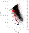 |
Fig. 1. Two-colour diagram i − Y vs. Y − K for the new sample. The large points are the known subdwarfs in the sample, listed in Table 5: blue circles show types sdM and sdL, and green squares show type esdL. The red open circles indicate sources with χ2 > 15 and E8 < 0.2. |
Catalogued subdwarfs in the M dwarf sample.
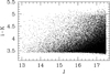 |
Fig. 2. Colour-magnitude diagram i − K vs. J for the new sample. |
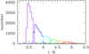 |
Fig. 3. Histograms of the distribution of i − K colours for each subtype, in half subtype bins, from M7 (left, violet) to M9.5 (right, red). |
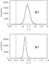 |
Fig. 4. Comparison of the colours of M7 dwarfs in the sample against the selection colour cuts. |
In this spectral range M7–M9.5, for each colour i − z, z − Y, Y − J, J − H, H − K, there is an approximately linear relation between colour and spectral type; the later types are redder. For this reason the stellar sequence presents a linear relation in a two-colour diagram. This is illustrated in Fig. 1, which plots i − Y versus Y − K. Therefore the i − K colour is the single colour most closely correlated with spectral type. In Fig. 2 we plot i − K versus J for the new sample. This figure illustrates the steep increase in number towards fainter magnitudes and the steep decrease in number counts towards redder colours. The colour i − K on its own provides a good measure of spectral type, as illustrated in Fig. 3, where the histograms of the i − K colour range of each spectral type are presented, showing little overlap between spectral types.
In the sample selection (Sect. 2), colour cuts i − z > 1.0, Y − J > 0.4 were applied before classifying. In Fig. 4 we plot histograms of these two colours for the earliest spectral classification in the sample, M7, i.e. plotting the bluest objects in the new sample. It is clear from both histograms that the number of sources lost from applying these colour cuts is negligible.
The numbers of sources broken down into half subtype bins are listed in Table 4. The numbers of sources per full spectral bin (e.g. M7 and M7.5 are combined as M7) are plotted against spectral type and compared against the counts of L dwarfs from Skrzypek et al. (2016), which are for the same area and magnitude cuts. The numbers decline towards later spectral types. The decline is steeper for the late M dwarfs and less steep for the L dwarfs. There is a break in the slope that occurs at L0. We assume a functional form N = 10a − bs, i.e. the counts are linear in log10. In this case s is spectral type, numbering M7 as 7 to L9 as 19, and a and b are constants. We fit to the counts separately for M7–L0 and for L0–L9, finding bM = 0.57 for the range M7–L0, and bL = 0.25 for the range L0–L9. These fits are plotted in Fig. 5.
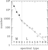 |
Fig. 5. Number counts of M7–9 dwarfs (solid symbols) compared to number counts for L dwarfs (open symbols) over the same area and depths. The dashed lines indicate the log-linear fits referred to in the text. |
There are a number of sources with large values of χ2, because the colours are a poor match to the templates. These sources are potentially interesting. The χ2 distribution for the sample is plotted in Fig. 6. Each SED has six data points and there are two parameters to fit: the brightness (i.e. overall normalisation) and the spectral type, leaving four degrees of freedom. Overplotted on the χ2 histogram is the theoretical χ2 distribution for four degrees of freedom. The curve is a reasonable fit, but the data are skewed to slightly smaller values, indicating that the uncertainties are slightly overestimated. The reason for the poor fit probably lies in the way the spread in the properties of the population has been modelled. In fitting templates to each SED, an additional uncertainty of 0.05 mag is added in quadrature to the photometric error in each band, to model the spread in each colour of the population, at each spectral type. This is a simplification, since it treats each band as independent, whereas the actual spread in colours is characterised by correlations between bands. The theoretical χ2 curve is nevertheless useful for comparison. If the errors were modelled perfectly, and the source list contained no peculiar objects, we would expect 158 (17) sources with χ2 > 15 (20), respectively, whereas the actual numbers are 298 (108) or 260 (87) if we exclude sources with E8 > 0.2, which are presumably peculiar because of the large reddening. With this in mind we selected χ2 > 20 as indicating that a source is peculiar, and the classifications are marked e.g. M7p. We scrutinised the images of these 108 sources in all bands, and it appears that all the sources are genuinely peculiar. Nevertheless it is in the nature of the selection to pick out sources with incorrect photometry, so there could be some remaining errors.
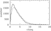 |
Fig. 6. Distribution of χ2 for the full sample compared to the theoretical distribution for 4 degrees of freedom. |
Several of the 87 peculiar (and not reddened) sources are known subdwarfs, including the two sources with the largest values of χ2 = 111 and 62. To investigate this further we matched the large sample of L subdwarfs in Table 1 of Zhang et al. (2018), as well as additional M subwdarfs in their Table 6, to our full sample. The 19 matched L subdwarfs and 2 matched M subdwarfs are listed in Table 5. Six of these are classified esdL, which are of lower metallicity than the sdL class (for details of the classification scheme, see Zhang et al. 2017). On average the photo-type classifications are two subtypes earlier than the correct spectral classification because of their unusual blue colours. Their colours are plotted in Fig. 1. The χ2 values for this sample range from 9 to 111 and have an average value of 32. Of the 21 matched subdwarfs, 15 have χ2 > 20, or 17% of the 87 peculiar sources that are not highly reddened. It would therefore be interesting to investigate further the remaining 72 sources. They might include subdwarfs missed by proper motion selection.
We can use the subdwarfs as a guide to estimate how many objects are significantly misclassified because of their peculiar colours. Of the 21 known subdwarfs, 19, that is nearly all, have χ2 > 15. The other two subdwarfs, with lower χ2, are misclassified by only 0.5 and 1 subtypes. There are only 260 sources in total with χ2 > 15, E8 < 0.2. These are plotted as red circles in Fig. 1. The majority, like the subdwarfs, lie to the left of the sequence visible in Fig. 1, but have on average less extreme colours. The selection χ2 > 15 therefore probably identifies nearly all sources misclassified by two subtypes or more, as well as intermediate objects. This suggests that the proportion of blue objects misclassified by two subtypes or more is safely less than 1%. The proportion of red circles lying to the right of the sequence in Fig. 1 is considerably smaller. These may represent dwarfs of spectral type earlier than M7 that are selected as M7 or later because they are peculiar and red.
The sample is limited to objects classified as point sources in UKIDSS. Point sources include unresolved binaries. A significant proportion of the sources appear in the Gaia DR2 catalogue and the parallaxes, combined with the apparent magnitudes in our catalogue, are useful to identify which sources are unresolved binaries. Any such objects in our sample with small values of χ2 are likely to be pairs of dwarfs of similar spectral type. Unresolved binaries with large χ2 may comprise a M dwarf primary and a secondary of later spectral type so that the colours are dominated by the primary. Another possibility is a M dwarf with a cool white dwarf (WD) companion. A large sample of M+WD binaries has been compiled by Rebassa-Mansergas et al. (2013) also using SDSS+UKIDSS. The majority of the M stars in their sample are M2 and M3. Therefore any white dwarfs in M+WD binaries found in our new sample might have different characteristics to the white dwarfs in their sample. The source ULAS J115908.00+103944.0, which is the object with the fifth largest value of χ2 in our sample, could be one example. The source was selected by SDSS for spectroscopic observation as a quasi-stellar object candidate, but the spectrum is classified M7 and displays excess blue continuum light. The colours of the source are such that it does not satisfy the selection criteria of Rebassa-Mansergas et al. (2013).
4. Precision of spectral types
We can establish the precision of the photo-type classifications by comparing them against classifications in the BUD sample (Schmidt et al. 2015) that was used to establish the relations between colour and spectral type in this range (Skrzypek et al. 2016). The precision of the classification impacts the number counts due to Eddington bias (Eddington 1913), i.e. the effect that because of the steep relation between counts and spectral type the uncertainty in classification scatters more objects from earlier to later classifications than vice versa. By establishing the precision it is then possible to correct the number counts for this effect.
The BUD classifications are measured to the nearest full subtype. The sample includes spectra of 11 820 M7–L8 dwarfs. We matched the M7 to M9 dwarfs in this sample to the classified parent sample of 404 496 sources (Sect. 2) from which our sample of M dwarfs is drawn, finding 3239 matches within the UKIDSS footprint and brighter than J = 17.5. To establish the precision it is important to match to the parent sample since some of the BUD M7 dwarfs are classified by photo-type as earlier than M7. We then measure the mean and scatter of the difference in classification, BUD minus photo-type. The histogram of differences is plotted in Fig. 7. The mean value for the 3239 dwarfs is 0.05 subtypes. Since we assume that the BUD classifications are in the mean correct, this establishes that the photo-type classifications are extremely accurate (systematic error). This is not surprising since, of course, the BUD sample itself was used to measure the template colours. The scatter in the differences establishes the precision (random error). The standard deviation of the differences in classification is just 0.6 subtypes. The same value is obtained whether the scatter is measured about the mean, or about zero, and whether the handful of sources with large differences in classification (greater than 2 subtypes) is clipped, or not.
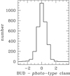 |
Fig. 7. Histogram of the difference in the classification between spectroscopy and using photo-type for the 3239 M7–M9 dwarfs from Schmidt et al. (2015) that matched the classified parent sample. |
This scatter is remarkably small considering that it is made up of three contributions added in quadrature: (1) the precision of photo-type; (2) the precision of the spectroscopic classifications; and (3) a contribution of  solely from the quantisation of the spectroscopic classifications into whole subtypes, rather than half subtypes. This means that both the photo-type and the spectroscopic classifications have a precision of better than 0.5 subtypes rms. This precision is as good as the precision of the best automated spectral classifiers (e.g. Christlieb et al. 2002). For a power-law slope of the number counts of 0.57 (Fig. 5), and a precision of 0.5 subtypes, the Eddington bias is at the level of 20%, i.e. the number counts are too large by a factor 1.2. Nevertheless it is debatable whether this calculation of Eddington bias has much meaning. If the sample had been obtained by a spectroscopic campaign with classifications to this precision it is unlikely any correction to the number counts would be deemed necessary, and therefore we ignore this correction in computing the LF.
5. Summary
In this paper we have presented a homogeneous sample of 33 665 bright J < 17.5 M7–M9.5 dwarfs, which have accurate spectral types obtained by applying the photo-type method to izYJHK SDSS and UKIDSS photometry. The effective area of the survey is 3070 deg2. The sample is of high S/N and low reddening. We took care to include, where possible, dwarfs that are located at small angular separations from bright stars. These may be binary companions to the bright stars, and are sometimes excluded in working with SDSS data. The sample is a companion to the sample of 1361 L and T dwarfs provided by Skrzypek et al. (2016), selected from the same multicolour dataset, and to the same depth. The number counts as a function of spectral type fall steeply over the range M7–M9.5 towards later types and there is a break at L0 to a flatter relation in the L dwarfs. For each source we list coordinates, izYJHK photometry, Galactic reddening, and the χ2 of the six-band photometric fit, in addition to the photo-type classification. The classifications are provided to the nearest half subtype and are precise to better than 0.5 subtypes rms. We argued that the precision is so good that Eddington bias in the number counts as a function of spectral type may be disregarded. The sources with large χ2 include subdwarfs, probably dwarfs of intermediate metallicity, and other peculiar types.
All the sources lie within a distance of 235 pc, so the sample will be useful for measuring the structure of the Milky Way disc close to the Galactic plane, and it will provide a new, more accurate, measurement of the space density of M7–M9.5 dwarfs. To measure the local space density we must measure the variation of the space density with height |z| from the Galactic plane and extrapolate to z = 0. The variation of the density of stars with height from the plane is often characterised using a  function (Spitzer 1942). The function is exponential e−|z|/zs at large heights but softens such that the central-plane density is reduced by a factor of four compared to the extrapolation to the central plane of the exponential distribution. While the sech2 function has been widely used, there is very little observational evidence of the actual softening near the Galactic plane. The new sample will be very useful to examine the form of the density distribution at small heights from the Galactic plane.
Revised template colours for M7–M9 dwarfs were published by Skrzypek et al. (2016).
Acknowledgments
This work was supported by Grant ST/N000838/1 from the Science and Technology Facilities Council. The UKIDSS project is defined in Lawrence et al. (2007). UKIDSS used the UKIRT Wide Field Camera (Casali et al. 2007). The photometric system is described in Hewett et al. (2006), and the calibration is described in Hodgkin et al. (2009). The science archive is described in Hambly et al. (2008). Funding for SDSS-III has been provided by the Alfred P. Sloan Foundation, the Participating Institutions, the National Science Foundation, and the U.S. Department of Energy Office of Science. The SDSS-III web site is http://www.sdss3.org/. SDSS-III is managed by the Astrophysical Research Consortium for the Participating Institutions of the SDSS-III Collaboration including the University of Arizona, the Brazilian Participation Group, Brookhaven National Laboratory, Carnegie Mellon University, University of Florida, the French Participation Group, the German Participation Group, Harvard University, the Instituto de Astrofisica de Canarias, the Michigan State/Notre Dame/JINA Participation Group, Johns Hopkins University, Lawrence Berkeley National Laboratory, Max Planck Institute for Astrophysics, Max Planck Institute for Extraterrestrial Physics, New Mexico State University, New York University, Ohio State University, Pennsylvania State University, University of Portsmouth, Princeton University, the Spanish Participation Group, University of Tokyo, University of Utah, Vanderbilt University, University of Virginia, University of Washington, and Yale University.
References
- Bochanski, J. J., Hawley, S. L., Covey, K. R., et al. 2010, AJ, 139, 2679 [NASA ADS] [CrossRef] [Google Scholar]
- Burgasser, A. J., Kirkpatrick, J. D., Brown, M. E., et al. 2002, ApJ, 564, 421 [NASA ADS] [CrossRef] [Google Scholar]
- Burgasser, A. J., Geballe, T. R., Leggett, S. K., Kirkpatrick, J. D., & Golimowski, D. A. 2006, ApJ, 637, 1067 [NASA ADS] [CrossRef] [Google Scholar]
- Casali, M., Adamson, A., & Alves de Oliveira, C. 2007, A&A, 467, 777 [NASA ADS] [CrossRef] [EDP Sciences] [Google Scholar]
- Chabrier, G. 2003, PASP, 115, 763 [NASA ADS] [CrossRef] [Google Scholar]
- Christlieb, N., Wisotzki, L., & Graßhoff, G. 2002, A&A, 391, 397 [NASA ADS] [CrossRef] [EDP Sciences] [Google Scholar]
- Covey, K. R., Hawley, S. L., Bochanski, J. J., et al. 2008, AJ, 136, 1778 [NASA ADS] [CrossRef] [Google Scholar]
- Cruz, K. L., Reid, I. N., Kirkpatrick, J. D., et al. 2007, AJ, 133, 439 [NASA ADS] [CrossRef] [Google Scholar]
- Delfosse, X., Forveille, T., Ségransan, D., et al. 2000, A&A, 364, 217 [NASA ADS] [Google Scholar]
- Dupuy, T. J., & Liu, M. C. 2012, ApJS, 201, 19 [NASA ADS] [CrossRef] [Google Scholar]
- Eddington, A. S. 1913, MNRAS, 73, 359 [Google Scholar]
- Ferguson, D., Gardner, S., & Yanny, B. 2017, ApJ, 843, 141 [NASA ADS] [CrossRef] [Google Scholar]
- Geballe, T. R., Knapp, G. R., Leggett, S. K., et al. 2002, ApJ, 564, 466 [NASA ADS] [CrossRef] [Google Scholar]
- Green, G. M., Schlafly, E. F., & Finkbeiner, D. 2018, MNRAS, 478, 651 [NASA ADS] [CrossRef] [Google Scholar]
- Hambly, N. C., Collins, R. S., Cross, N. J. G., et al. 2008, MNRAS, 384, 637 [NASA ADS] [CrossRef] [Google Scholar]
- Hawley, S. L., Covey, K. R., Knapp, G. R., et al. 2002, AJ, 123, 3409 [NASA ADS] [CrossRef] [Google Scholar]
- Hewett, P. C., Warren, S. J., Leggett, S. K., & Hodgkin, S. T. 2006, MNRAS, 367, 454 [NASA ADS] [CrossRef] [Google Scholar]
- Hodgkin, S. T., Irwin, M. J., Hewett, P. C., & Warren, S. J. 2009, MNRAS, 394, 675 [NASA ADS] [CrossRef] [Google Scholar]
- Kirkpatrick, J. D., Reid, I. N., Liebert, J., et al. 1999, ApJ, 519, 802 [NASA ADS] [CrossRef] [Google Scholar]
- Lawrence, A., Warren, S. J., Almaini, O., et al. 2007, MNRAS, 379, 1599 [NASA ADS] [CrossRef] [MathSciNet] [Google Scholar]
- Martín, E. L., Delfosse, X., Basri, G., et al. 1999, AJ, 118, 2466 [NASA ADS] [CrossRef] [Google Scholar]
- Rebassa-Mansergas, A., Agurto-Gangas, C., Schreiber, M. R., Gänsicke, B. T., & Koester, D. 2013, MNRAS, 433, 3398 [NASA ADS] [CrossRef] [Google Scholar]
- Schmidt, S. J., West, A. A., Hawley, S. L., & Pineda, J. S. 2010, AJ, 139, 1808 [NASA ADS] [CrossRef] [Google Scholar]
- Schmidt, S. J., Hawley, S. L., West, A. A., et al. 2015, AJ, 149, 158 [NASA ADS] [CrossRef] [Google Scholar]
- Skrutskie, M. F., Cutri, R. M., Stiening, R., et al. 2006, AJ, 131, 1163 [NASA ADS] [CrossRef] [Google Scholar]
- Skrzypek, N., Warren, S. J., Faherty, J. K., et al. 2015, A&A, 574, A78 [Google Scholar]
- Skrzypek, N., Warren, S. J., & Faherty, J. K. 2016, A&A, 589, A49 [NASA ADS] [CrossRef] [EDP Sciences] [Google Scholar]
- Spitzer, Jr., L. 1942, ApJ, 95, 329 [NASA ADS] [CrossRef] [Google Scholar]
- Strauss, M. A., Fan, X., Gunn, J. E., et al. 1999, ApJ, 522, L61 [NASA ADS] [CrossRef] [Google Scholar]
- Tonry, J. L., Stubbs, C. W., Lykke, K. R., et al. 2012, ApJ, 750, 99 [NASA ADS] [CrossRef] [Google Scholar]
- West, A. A., Hawley, S. L., Bochanski, J. J., et al. 2008, AJ, 135, 785 [NASA ADS] [CrossRef] [Google Scholar]
- West, A. A., Morgan, D. P., Bochanski, J. J., et al. 2011, AJ, 141, 97 [NASA ADS] [CrossRef] [Google Scholar]
- York, D. G., Adelman, J., Anderson, Jr., J. E., et al. 2000, AJ, 120, 1579 [CrossRef] [Google Scholar]
- Zhang, Z. H., Pinfield, D. J., Gálvez-Ortiz, M. C., et al. 2017, MNRAS, 464, 3040 [NASA ADS] [CrossRef] [Google Scholar]
- Zhang, Z. H., Galvez-Ortiz, M. C., Pinfield, D. J., et al. 2018, MNRAS, 480, 5447 [NASA ADS] [CrossRef] [Google Scholar]
All Tables
Solid angle of survey as a function of Galactic latitude. The area is zero at angles not listed.
All Figures
|
Fig. 1. Two-colour diagram i − Y vs. Y − K for the new sample. The large points are the known subdwarfs in the sample, listed in Table 5: blue circles show types sdM and sdL, and green squares show type esdL. The red open circles indicate sources with χ2 > 15 and E8 < 0.2. |
| In the text | |
|
Fig. 2. Colour-magnitude diagram i − K vs. J for the new sample. |
| In the text | |
|
Fig. 3. Histograms of the distribution of i − K colours for each subtype, in half subtype bins, from M7 (left, violet) to M9.5 (right, red). |
| In the text | |
|
Fig. 4. Comparison of the colours of M7 dwarfs in the sample against the selection colour cuts. |
| In the text | |
|
Fig. 5. Number counts of M7–9 dwarfs (solid symbols) compared to number counts for L dwarfs (open symbols) over the same area and depths. The dashed lines indicate the log-linear fits referred to in the text. |
| In the text | |
|
Fig. 6. Distribution of χ2 for the full sample compared to the theoretical distribution for 4 degrees of freedom. |
| In the text | |
|
Fig. 7. Histogram of the difference in the classification between spectroscopy and using photo-type for the 3239 M7–M9 dwarfs from Schmidt et al. (2015) that matched the classified parent sample. |
| In the text | |
Current usage metrics show cumulative count of Article Views (full-text article views including HTML views, PDF and ePub downloads, according to the available data) and Abstracts Views on Vision4Press platform.
Data correspond to usage on the plateform after 2015. The current usage metrics is available 48-96 hours after online publication and is updated daily on week days.
Initial download of the metrics may take a while.