| Issue |
A&A
Volume 623, March 2019
|
|
|---|---|---|
| Article Number | A95 | |
| Number of page(s) | 5 | |
| Section | The Sun | |
| DOI | https://doi.org/10.1051/0004-6361/201834299 | |
| Published online | 11 March 2019 | |
UV core dimming in coronal streamer belt and the projection effects⋆
1
INAF – Astrophysical Observatory of Torino, Via Osservatorio 20, 10025 Pino Torinese, Italy
e-mail: This email address is being protected from spambots. You need JavaScript enabled to view it.
2
Department of Physics, Catholic University of America, Washington, DC 20064, USA
3
NASA Goddard Space Flight Center, Code 671, Greenbelt, MD 20771, USA
4
Visiting, Department of Geosciences, Tel Aviv University, Tel Aviv, Israel
Received:
21
September
2018
Accepted:
14
January
2019
Abstract
During solar minimum activity, the coronal structure is dominated by a tilted streamer belt, associated with the sources of the slow solar wind. It is known that some UV coronal spectral observations show a quite evident core dimming in heavy ions emission in quiescent streamers. In this paper, our purpose is to investigate this phenomenon by comparing observed and simulated UV coronal ion spectral line intensities. First, we computed the emissivities and the intensities of HI Lyα and OVI spectral lines starting from the physical parameters of a time-dependent 3D three-fluid MHD model of the coronal streamer belt. The model is applied to a tilted dipole (10°) solar minimum magnetic structure. Next, we compared the results obtained from the model in the extended corona (from 1.5 to 4 R⊙) to the UV spectroscopic data from the Ultraviolet Coronagraph Spectrometer (UVCS) onboard SOHO during the minimum of solar activity (1996). We investigate the line-of-sight integration and projection effects in the UV spectroscopic observations, disentangled by the 3D multifluid model. The results demonstrate that the core dimming in heavy ions is produced by the physical processes included in the model (i.e., combination of the effects of heavy ion gravitational settling, and energy exchange of the preferentially heated heavy ions through the interaction with electrons and protons) but it is visible only in some cases where the magnetic structure is simple, such as a (tilted) dipole.
Key words: Sun: corona / solar wind / Sun: UV radiation / magnetohydrodynamics (MHD)
Movie associated to Fig. 3 is available at https://www.aanda.org
© ESO 2019
1. Introduction
The slow solar wind is an important component of solar activity affecting heliospheric conditions. Since the origin of the slow solar wind is not well understood and it is still intensively studied (see recent review by Abbo et al. 2016), data from the Ultraviolet Coronagraph Spectrometer (UVCS) onboard SOHO can be crucial for this topic. One of the first results of UVCS was the discovery that, during solar minimum activity, quiescent streamers may show a marked heavy ion (such as O5+, Mg9+, and Si11+) depletion in their cores with respect to their bright lateral branches (e.g., Noci et al. 1997b; Marocchi et al. 2001; Uzzo et al. 2003). In the last 20+ years, several authors have proposed different interpretations of this result, which also relate to the slow solar wind origin (e.g., Noci et al. 1997a; Raymond et al. 1997; Ofman 2000; Frazin et al. 2003; Akinari 2007). In the present work, we have studied the importance of the line-of-sight (LOS) observational aspects of the streamers in the plane of the sky (POS), due to the presence of a tilted coronal streamer belt appropriate near solar minimum activity conditions. Figure 1 shows an example of this feature and in particular that the same streamer observed in HI Lyα 1216 Å line (left panel) and in OVI 1032 Å line (central panel) look different: the ion image has a bifurcated structure and seem to consist of two or three sub-streamers at low heliocentric distances; on the other hand, the HI Lyα image has a much simpler structure with maximum brightness on the axis. The intensity profiles along the slit at 1.89 R⊙ shown in the right panel highlights the observation of the core dimming due to O5+ ion emission. In a previous analyses, we have studied the streamer core dimming in Mg9+ ion emission which is less evident than in O5+ ion emission (Ofman et al. 2013). In order to investigate the observational heavy-ion emission dimming effect, the comparison between data analysis and numerical models is needed. Multifluid models were used in the past to study the EUV emission with assumption of azimuthal symmetry (i.e., 2.5D models; see, e.g., Ofman 2000; Ofman et al. 2011, 2013). We note that due to the low heavy ion abundance the effect of either O5+ or Mg9+ on the streamer structure in electrons and protons is small. However, the heavy ion abundances variation and outflow properties are strongly affected by the electron-proton and magnetic field streamer structure, as evident from the results of the three-fluid models. The first 3D multifluid model was applied to the tilted dipole streamer belt configuration in a computational study (Ofman et al. 2015). In the present paper, for the first time we have used the 3D multifluid simulation results to model streamers that contain heavy ions in addition to protons and electrons to calculate the ion emission, while traditional single fluid magneto-hydrodynamic (MHD) models cannot capture the significantly different properties, interactions, and dynamics of the various ions. In this way, we are able to evaluate the ion-dependent projection effects by studying the importance of the integration along the LOS of the streamer structures.
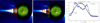 |
Fig. 1. Composite solar images of an equatorial streamer observed from August 30 to September 2, 1996 at east limb. The disk is imaged with EIT/SOHO in the Fe XII 195 Å line. The limb images are obtained with the LASCO/SOHO C2 coronagraph. The slit (IFOV) of UVCS is superposed to the coronal images in HI Lyα 1216 Å line (left panel) and in OVI 1032 Å line (central panel). Right panel: intensity profiles along the slit at 1.89 R⊙ of HI Lyα 1216 Å line (black line) and of OVI 1032 Å line (blue line). The core dimming in OVI spectral line emission is evident. |
2. Observations and data analysis
UVCS has been a fundamental instrument for the study of the extended solar corona, specially designed for the solar wind velocity and composition. The streamer and the regions adjacent to the streamer belt during solar minimum activity have been studied in detail through the UVCS observations in the past and there are numerous papers concerning this topic (e.g., Strachan et al. 2002; Antonucci et al. 2005; Susino et al. 2008; Abbo et al. 2010). Also in the first results papers of UVCS data, many important aspects of the streamer belt observed in the UV lines were reported (e.g., Kohl et al. 1997; Raymond et al. 1997; Antonucci et al. 1997; Strachan et al. 1997). Such data are still unique (in the distance range from 1.5 to 4 R⊙) and are therefore very important for studying the slow solar wind origin in the corona. Indeed, extended coronal spectroscopic data are not yet available after UVCS operational period since there is no other spectro-coronagraph instrument in the ultraviolet solar spectrum that can observe out to several solar radii above the photosphere. Moreover, the 1996–1997 UVCS data correspond to deep minimum of solar activity, since the morphology and the magnetic structure are quite similar to a dipole without anomalies, compared to the more complex recent minimum of 2006–2007. Therefore, these data are good candidates for comparison with the physical parameters obtained using the 3D multifluid model of relatively simple tilted dipole streamer belt structure applied in this work. The main spectral lines detected with UVCS are the OVI doublet lines at 1031.93 and 1037.62 Å and the HI Lyman α line at 1216 Å in two channels, respectively 984–1080 Å and 1100–1361 Å spectral ranges. In particular, in this work we have analysed the UVCS observations in the period August 1 to September 2, 1996 in the altitude range from 1.5 to 3.5 R⊙. We have studied only the equatorial streamer belt with a latitude from about 65° to 130° at the east limb and from 245° to 340° at the west limb (counterclockwise from the north pole). Each day the observation was performed in approximately 9–12 h and scanned a part of the corona corresponding of about 60°, and the spectrometer slit was about 40′ long. The counts detected by the instrument of the different spectral lines were corrected for stray light and transformed to intensity I(λ) by applying the standard radiometric calibration by Gardner et al. (1996). The spectral line profiles I(λ) were fitted with a Gaussian function, that represents the solar line profile, convolved with a Voigt curve and an appropriate function that account for the instrumental broadening and the width of the spectrometer slit, respectively. The function resulting from the convolution was added to a background linearly dependent on wavelength. The parameters defining the instrumental Voigt function and the corrections for stray light are those derived according to the method in Giordano (1998). The line intensity was obtained by integrating over the solar line profile.
3. Three-dimensional multifluid MHD model of a tilted dipole
The model of coronal streamer belt includes O5+ ions as one of the fluids, with proton and massless electron fluids. Other ions, such as He++ and Mg9+ were modeled with a multifluid model as well previously (see the review by Abbo et al. 2016). We would like to point out that the effect of the O5+ ions on the electron and proton streamer structure is negligible, primarily due to the low relative abundance of the heavy ions. In fact, by comparing the electron and proton streamer structures in the three-fluid 2.5D model with O5+ (see Fig. 4 in Ofman et al. 2011) and the three-fluid model results with Mg9+ – two orders of magnitude less abundant than O5+ (see Figs. 3 and 4 in Ofman et al. 2013), it is evident that the electron-proton streamers are very similar in the two models. The time-dependent 2.5D three-fluids MHD model is based on equations with full ion dynamics as described by Ofman (2000, 2004a,b); Ofman et al. (2011; see the review by Abbo et al. 2016). The model was extended to full 3D multifluid and applied to a tilted dipole (10° tilt with respect to the solar rotation axis) solar minimum magnetic structure, described in detail by Ofman et al. (2015). The above references include the full set of the three-fluid equations with gravity, Coulomb friction terms, and energy exchange terms, as well as the discussion of the boundary and initial conditions (see, e.g., Sect. 2 in Ofman et al. 2015). In the present study we used the published 3D three-fluid model results to calculate the emissivities. For convenience, we describe briefly the model setup: the three-fluid model equations assume quasi-neutrality, massless electrons in non-relativistic plasma, and solve the continuity and momentum equations for the ions with thermal and gravity forces, collisional couplings and electromagnetic couplings through the Lorentz forces. The electrons are treated as massless fluid leading to the generalized Ohm’s law. We solved three coupled energy equations that include collisional energy exchanges between the species and heating terms supplemented with polytropic equations of states for each species, and the inductance equation. The model was initialized with a tilted dipole magnetic field with initially hydrostatic ion density structure and boundary conditions at r = 1 R⊙ with fixed magnetic field while the values of density, temperature and velocity components adjust self-consistently approximating incoming characteristics. At the outer boundary, the conditions were open allowing solar wind outflow as described in detail in Ofman et al. (2015). The model was run until a streamer with appropriate self-consistent current sheet was formed and reaches a quasi-steady state. In Fig. 2, the magnetic field lines of the modeled streamer are shown: the field lines are closed in the core of the streamer and open in the adjacent regions due to the effects of thermal pressure in agreement with past streamer studies (see the review, Abbo et al. 2016).
 |
Fig. 2. Three-dimensional structure of the coronal magnetic field in the steady-state solution showing formation of a streamer belt from the initial tilted dipole magnetic field configuration. The coordinate system is shown in the top right corner (adapted from Ofman et al. 2015). |
It has been shown previously that the 2.5D multifluid model results (such as O5+ density structure, temperatures, and outflow speeds), are in qualitative agreement with UVCS observations (Ofman 2000, 2004a; Ofman et al. 2011, 2013). Here we extend the comparison by using 3D three-fluid model with more realistic three-dimensional setup than in past studies, allowing temperature coupling in the energy equations with polytropic index γ = 1.05 for all species (in Ofman 2000 model the O5+ were set to be isothermal). In the present study we have modeled the slow solar wind and do not include the additional sources of momentum required to produce the fast wind (as considered in coronal holes, e.g., in Ofman 2004a).
From the 3D three-fluid MHD model, we have derived the coronal structure of the following physical parameters in the streamer belt: values of electron and proton temperatures, electron and oxygen ion density and outflow velocity of electron, proton and oxygen ions.
4. Computation of spectral lines emissivities and intensities
The physical parameters obtained from the 3D three-fluid MHD model are used to compute the expected emissivity from HI Lyα and OVI 1032 Å spectral lines. The multifluid model provides maps of values for a full set of coronal parameters, such as temperatures, densities, and ion outflow velocities which enables the computations of maps of UV emission from the solar corona. There are two main mechanisms contributing to the formation of a UV coronal line: the resonant scattering of radiation coming from the bright solar disk by ions in the outer corona and the collisional excitation by electron impact on ions followed by radiative decay. Therefore, the total emissivity coming from an optically thin corona is the combination of the resonant, jres, and collisional, jcoll, emissivities: j = jres + jcoll. The two components have been computed following the expressions by Noci et al. (1987). In our computation we assumed uniformly bright exciting radiation coming from the solar disk, in particular for HI Lyα we adopted the SUMER profile observed at solar minimum in 1996 July (Lemaire et al. 2002) and for OVI 1032 the intensity reported by Wilhelm et al. (1998) and the line width by Warren et al. (1997).
The HI and OVI simulated emissivities have been computed using the plasma parameters obtained from the results of the three-fluid model of the streamer belt at solar minimum. Two cubes of emissivities values have been obtained with 256 elements in each dimension, one for HI Lyα line and one for OVI 1032 line. In order to derive the spectral lines intensity maps from the model, the integration along the LOS has been then performed. Since the 3D solar corona is not symmetric due to the presence of the tilt with respect to the solar rotation axis, the choice of observing direction is crucial. We have computed the HI Lyα and OVI intensities by rotating the cube of the emissivities in steps of one degree, and by summing the values along the LOS. As an example, in Fig. 3, two intensity images of the entire corona (excluding the polar regions) for longitude of 240° are shown at the top: HI Lyα intensity map (left), OVI 1032 intensity map (right). The normalized latitudinal cuts of intensity at 3 R⊙ along the slit (dashed white line in the top panels of Fig. 3) for HI Lyα (black) and OVI 1032 (red) lines are shown in the bottom panels of Fig. 3 at 0°, 90° and 240° of longitude, respectively. The evolution of HI Lyα intensity map, OVI 1032 intensity map and the latitudinal cuts at 3 R⊙ along the slit as a function of longitude is shown in a movie available online. It is evident the effect of the tilt angle of the streamer belt in both of the intensity images (and movies), but we notice the presence of the core dimming in the streamer belt clearly only in some of the OVI latitudinal cuts (i.e., at 90° and 240°) and not in the HI Lyα ones. These cases confirm the observational examples shown in Fig. 1.
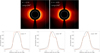 |
Fig. 3. Top panel: intensity images computed from the model at 240° of longitude: HI Lyα intensity map (left panel), OVI 1032 intensity map (right panel). Bottom panel: normalized intensity profiles at 0°, 90° and 240° of longitude at 3 R⊙ along the slit (dashed white line in the top panels): HI Lyα intensity profile (black) and OVI 1032 intensity profile (red). See also the movie available online. |
In order to clarify the comparison between the observations and the model results, we have reconstructed Carrington maps (latitude as a function of time or longitude) of the intensities observed by UVCS and computed from the model. The Carrington maps of the spectral lines observed at 1.7 R⊙ in the period August 1–18, 1996, are shown in the top panels of Fig. 4 (left panel: HI Lyα; right panel: OVI 1032). They are built by extracting a profile of each coronal image reconstructed from UVCS spectral data at a certain radial distance from the Sun center (in this case about 1.7 R⊙), then we have piled them up; in this way, each column represents one image of one day. The dotted line shows the neutral line as computed by Wilcox Solar Observatory in the “classical” approximation which locates the source surface at 2.5 R⊙. The position of the neutral line follows mostly the HI Lyα peak line and the dimming of ion intensity. The core dimming is clear in the OVI map only for some longitudes. In other cases the HI and OVI intensity peaks are, approximately, at the same latitude.
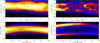 |
Fig. 4. Top panel: Carrington maps (latitude as a function of longitude or time) of the intensities of HI Lyα (left panel) and OVI 1032 (right panel) spectral lines observed by UVCS in the period August 1–18, 1996 at 1.7 R⊙ (normalized units). The dotted black (left panel) or white (right panel) line shows the neutral line as computed by Wilcox Solar Observatory. Bottom panel: Carrington maps (latitude as a function of longitude) of the computed intensities from the model for the same spectral lines at 1.7 R⊙ (normalized units). |
From the model, we have built a 14-day (half rotation) Carrington map of HI and OVI intensity by rotating the 3D emissivity cubes of steps by one degree and then integrating along different LOS. The results are shown in the bottom panels of Fig. 4 in normalized units.
5. Discussion
From the comparison of the Carrington maps obtained from the observations (Fig. 4 – top panels) and from the model (Fig. 4 – bottom panels), there is a reasonably good agreement in the general trend of the spectral intensities, even though the initial conditions of the magnetic field are based on an idealized tilted dipole model. In the simulation, the OVI core dimming varies in latitudinal width depending on the projection effects: for longitudes around 0° the core dimming is very faint, whereas around 90° it is well marked. In the observations, the OVI core dimming is concentrated in about 20° of latitude range, which is a much less width than in the model. The interesting result of this work is that the core dimming in heavy ions is produced by the physical processes included in the model (i.e., combination of the effects of heavy ion gravitational settling, and energy exchange of the preferentially heated heavy ions through the interaction with electrons and protons) but it is visible only in some cases due to projection effects of multiple structures streamer and due to the tilted magnetic dipole. The present study demonstrates the effects of the tilt between the streamer belt axis and the solar rotation axis on the observed streamer structure and core dimming in the OVI emission in the POS. The core dimming observed in heavy ions (e.g., O5+ and Mg9+ emissions) was already discussed and compared with the UVCS observations by using a 2.5 MHD (i.e., with azimuthal symmetry) multifluid model (Ofman et al. 2011, 2013). However, in this work we stress the importance of the tilt angle and we clarify the effects of the integration along the LOS that can only be modeled with more realistic full 3D multifluid model. In a future study, we would like to investigate the importance of different tilted angles on the results, by initializing the model with more complex and realistic magnetic geometry that corresponds to solar maximum conditions.
Movie
Movie of Fig. 3 Access Supplementary Material
Acknowledgments
UVCS is a joint project of the National Aeronautics and Space Administration (NASA), the Agenzia Spaziale Italiana (ASI) and Swiss Founding Agencies. LO would like to acknowledge support by NASA Cooperative agreement NNG11PLA10A2 670.154 to CUA. Resources supporting this work were provided by the NASA High-End Computing (HEC) Program through the NASA Advanced Supercomputing (NAS) Division at Ames Research Center.
References
- Abbo, L., Antonucci, E., Mikić, Z., et al. 2010, AdSpR, 46, 1400 [NASA ADS] [Google Scholar]
- Abbo, L., Ofman, L., Antiochos, S. K., et al. 2016, Space Sci. Res., 201, 55 [Google Scholar]
- Akinari, N. 2007, ApJ, 668, 1196 [NASA ADS] [CrossRef] [Google Scholar]
- Antonucci, E., Giordano, S., Benna, C., et al. 1997, in Fifth SOHO Workshop: The Corona and Solar Wind Near Minimum Activity, ed. A. Wilson, ESA SP, 404, 75 [NASA ADS] [Google Scholar]
- Antonucci, E., Abbo, L., & Dodero, M. A. 2005, A&A, 435, 699 [NASA ADS] [CrossRef] [EDP Sciences] [Google Scholar]
- Frazin, R. A., Cranmer, S. R., & Kohl, J. L. 2003, ApJ, 597, 1145 [NASA ADS] [CrossRef] [Google Scholar]
- Gardner, L. D., Kohl, J. L., Daigneau, P. S., et al. 1996, in Ultraviolet Atmospheric and Space Remote Sensing: Methods and Instrumentation, eds. R. E. Huffman, & C. G. Stergis, Proc. SPIE, 2831, 2 [NASA ADS] [CrossRef] [Google Scholar]
- Giordano, S. 1998, PhD Thesis, Univ. Torino [Google Scholar]
- Kohl, J. L., Noci, G., Antonucci, E., et al. 1997, Sol. Phys., 175, 613 [NASA ADS] [CrossRef] [Google Scholar]
- Lemaire, P., Emerich, C., Vial, J. C., et al. 2002, in From Solar Min to Max: Half a Solar Cycle with SOHO, A. Wilson, ESA SP, 508, 219 [NASA ADS] [Google Scholar]
- Marocchi, D., Antonucci, E., & Giordano, S. 2001, Ann. Geophys., 19, 135 [NASA ADS] [CrossRef] [Google Scholar]
- Noci, G., Kohl, J. L., & Withbroe, G. L. 1987, ApJ, 315, 706 [NASA ADS] [CrossRef] [Google Scholar]
- Noci, G., Kohl, J. L., Antonucci, E., et al. 1997a, in Fifth SOHO Workshop: The Corona and Solar Wind Near Minimum Activity, ed. A. Wilson, ESA SP, 404, 75 [NASA ADS] [Google Scholar]
- Noci, G., Kohl, J. L., Antonucci, E., et al. 1997b, AdSpR, 20, 2219 [Google Scholar]
- Ofman, L. 2000, Geophys. Res. Lett., 27, 2885 [NASA ADS] [CrossRef] [Google Scholar]
- Ofman, L. 2004a, AdSpR, 33, 681 [NASA ADS] [Google Scholar]
- Ofman, L. 2004b, J. Geophys. Res. (Space Phys.), 109, 7102 [NASA ADS] [CrossRef] [Google Scholar]
- Ofman, L., Abbo, L., & Giordano, S. 2011, ApJ, 734, 30 [NASA ADS] [CrossRef] [Google Scholar]
- Ofman, L., Abbo, L., & Giordano, S. 2013, ApJ, 762, 18 [NASA ADS] [CrossRef] [Google Scholar]
- Ofman, L., Provornikova, E., Abbo, L., & Giordano, S. 2015, Ann. Geophys., 33, 47 [NASA ADS] [CrossRef] [Google Scholar]
- Raymond, J. C., Kohl, J. L., Noci, G., et al. 1997, Sol. Phys., 175, 645 [NASA ADS] [CrossRef] [Google Scholar]
- Strachan, L., Raymond, J. C., Panasyuk, A. V., et al. 1997, in Fifth SOHO Workshop: The Corona and Solar Wind Near Minimum Activity, ed. A. Wilson, ESA SP, 404, 691 [NASA ADS] [Google Scholar]
- Strachan, L., Suleiman, R., Panasyuk, A. V., Biesecker, D. A., & Kohl, J. L. 2002, ApJ, 571, 1008 [Google Scholar]
- Susino, R., Ventura, R., Spadaro, D., Vourlidas, A., & Landi, E. 2008, A&A, 488, 303 [NASA ADS] [CrossRef] [EDP Sciences] [Google Scholar]
- Uzzo, M., Ko, Y.-K., Raymond, J. C., Wurz, P., & Ipavich, F. M. 2003, ApJ, 585, 1062 [NASA ADS] [CrossRef] [Google Scholar]
- Warren, H. P., Mariska, J. T., Wilhelm, K., & Lemaire, P. 1997, ApJ, 484, L91 [NASA ADS] [CrossRef] [Google Scholar]
- Wilhelm, K., Marsch, E., Dwivedi, B. N., et al. 1998, ApJ, 500, 1023 [NASA ADS] [CrossRef] [Google Scholar]
All Figures
|
Fig. 1. Composite solar images of an equatorial streamer observed from August 30 to September 2, 1996 at east limb. The disk is imaged with EIT/SOHO in the Fe XII 195 Å line. The limb images are obtained with the LASCO/SOHO C2 coronagraph. The slit (IFOV) of UVCS is superposed to the coronal images in HI Lyα 1216 Å line (left panel) and in OVI 1032 Å line (central panel). Right panel: intensity profiles along the slit at 1.89 R⊙ of HI Lyα 1216 Å line (black line) and of OVI 1032 Å line (blue line). The core dimming in OVI spectral line emission is evident. |
| In the text | |
|
Fig. 2. Three-dimensional structure of the coronal magnetic field in the steady-state solution showing formation of a streamer belt from the initial tilted dipole magnetic field configuration. The coordinate system is shown in the top right corner (adapted from Ofman et al. 2015). |
| In the text | |
|
Fig. 3. Top panel: intensity images computed from the model at 240° of longitude: HI Lyα intensity map (left panel), OVI 1032 intensity map (right panel). Bottom panel: normalized intensity profiles at 0°, 90° and 240° of longitude at 3 R⊙ along the slit (dashed white line in the top panels): HI Lyα intensity profile (black) and OVI 1032 intensity profile (red). See also the movie available online. |
| In the text | |
|
Fig. 4. Top panel: Carrington maps (latitude as a function of longitude or time) of the intensities of HI Lyα (left panel) and OVI 1032 (right panel) spectral lines observed by UVCS in the period August 1–18, 1996 at 1.7 R⊙ (normalized units). The dotted black (left panel) or white (right panel) line shows the neutral line as computed by Wilcox Solar Observatory. Bottom panel: Carrington maps (latitude as a function of longitude) of the computed intensities from the model for the same spectral lines at 1.7 R⊙ (normalized units). |
| In the text | |
Current usage metrics show cumulative count of Article Views (full-text article views including HTML views, PDF and ePub downloads, according to the available data) and Abstracts Views on Vision4Press platform.
Data correspond to usage on the plateform after 2015. The current usage metrics is available 48-96 hours after online publication and is updated daily on week days.
Initial download of the metrics may take a while.