| Issue |
A&A
Volume 623, March 2019
|
|
|---|---|---|
| Article Number | A91 | |
| Number of page(s) | 8 | |
| Section | Astrophysical processes | |
| DOI | https://doi.org/10.1051/0004-6361/201833697 | |
| Published online | 12 March 2019 | |
Gamma rays from red giant wind bubbles entering the jets of elliptical host blazars
Departament de Física Quàntica i Astrofísica, Institut de Ciències del Cosmos (ICC), Universitat de Barcelona (IEEC-UB), Martí i Franquès 1, 08028 Barcelona, Spain
e-mail: This email address is being protected from spambots. You need JavaScript enabled to view it.
Received:
21
June
2018
Accepted:
29
January
2019
Abstract
Context. Blazars in elliptical hosts have a population of red giants surrounding their jet. These stars can carry large wind-blown bubbles into the jets, leading to gamma-ray emission through bubble-jet interactions.
Aims. We study the interaction dynamics and the gamma-ray emission produced when the bubbles formed by red giant winds penetrate the jet of a blazar in an elliptical galaxy.
Methods. First, we characterized the masses and penetration rates of the red giant wind bubbles that enter the jet. Then, the dynamical evolution of these bubbles under the jet impact was analysed analytically and numerically, and the radiation losses of the particles accelerated in the interaction were characterised. Finally, the synchrotron and the inverse Compton contributions above ∼100 MeV were estimated under different jet magnetic fields, powers, and Lorentz factors.
Results. We find that an analytical dynamical model is a reasonable approximation for the red giant wind bubble-jet interaction. The radiation produced by these wind bubbles interacting with a jet can have a duty cycle of up to ∼1. For realistic magnetic fields, gamma rays could be detectable from sources within the local universe, preferentially from those with high Lorentz factors (∼10), and this could be a relatively common phenomenon for these sources. For magnetic fields in equipartition with the jet power, and high acceleration rates, synchrotron gamma rays may be detectable even for modest Lorentz factors (∼3), but with a much lower duty cycle.
Conclusions. Blazars in elliptical galaxies within the local universe can produce detectable transient or persistent gamma-ray emission from red giant wind bubbles entering their jets.
Key words: radiation mechanisms: non-thermal / galaxies: active / galaxies: nuclei / galaxies: jets
© ESO 2019
1. Introduction
Supermassive black holes, present in the innermost regions of galaxies, may accrete the material surrounding them, becoming active galactic nuclei (AGN). Some AGN produce collimated relativistic outflows, or jets (e.g. Begelman et al. 1984), which propagate through the host galaxy. This propagation will inevitably lead to the jet interacting with a variety of obstacles including stars, gas, and dense clouds. These interactions may affect the jet dynamically (e.g. Blandford & Koenigl 1979; Wang et al. 2000; Sutherland & Bicknell 2007). In particular, stars with high mass-loss rates may load the jet with enough matter to result in deceleration (e.g. Komissarov 1994; Bowman et al. 1996; Hubbard & Blackman 2006; Bosch-Ramon et al. 2012; Perucho et al. 2014, 2017).
The winds of stars interacting with AGN jets produce a double bow-shock structure in which particles can be accelerated to relativistic energies, possibly contributing to the jet’s total non-thermal emission. Several works have explored this interaction and the resulting emission, both in the case of steady radiation and transient events (e.g. Bednarek & Protheroe 1997; Barkov et al. 2010, 2012; Khangulyan et al. 2013; Araudo et al. 2013; Bednarek & Banasiński 2015; Wykes et al. 2015; Bosch-Ramon 2015; de la Cita et al. 2016; Vieyro et al. 2017), with results that often point towards possible detectability for nearby sources.
Previous works have considered persistent emission being generated from a whole population of stars, though in all cases they focus on the interaction that occurs within the jet once the star has already penetrated (Araudo et al. 2013; Wykes et al. 2015; Bosch-Ramon 2015; Vieyro et al. 2017). We refer to this stage of interaction as “steady state”.
In this work, we focus on the possible mass-loading and emission generated at the moment when stars penetrate the jet, and the latter interacts with large “bubbles” of material formed by the collision between the stellar wind and the interstellar medium. Perucho et al. (2017) inferred possible significant non-thermal emission and mass-loading from this early stage in jet-star interaction, using 2D and 3D simulations of one single star with heavy mass loss. We use semi-analytical prescriptions to estimate if this is the case for a whole population of stars within a galaxy.
We focus here on the study of blazar sources, as Doppler boosting is an important factor in enhancing the resulting emission. We consider only low-luminosity sources (i.e. Lj = 1043 − 1045 erg s−1), more abundant in the local universe. As recent studies show that the preferred hosts of blazars are late-type galaxies (e.g. Scarpa et al. 2000; Nilsson et al. 2003; Falomo et al. 2014; Olguín-Iglesias et al. 2016), we model the red giant population within an elliptical bulge. A mostly phenomenological approach is adopted (with the exception of an illustrative numerical simulation), based on specific source knowledge and reference parameter values, as a first simplified step to explore the outcome of the wind bubble and jet interaction.
The paper is organized as follows. A description of the prescriptions used to characterize the stellar population is given in Sect. 2. In Sect. 3, the properties of the stellar bubbles outside and immediately after penetrating the jet are described. The bubble evolution within the jet is described through analytical estimates and compared with simulation results in Sect. 4. Then, the non-thermal emission generated by bubble-jet interactions is estimated in Sect. 5. Finally, the discussion is presented in Sect. 6.
2. Characterization of the stellar population in an elliptical galaxy
Elliptical galaxies contain large populations of red giants, which can have high mass-loss rates, in the range of Ṁ ∼ 10−10 − 10−5 M⊙ yr−1 (Reimers 1975). We model the red giant population of any elliptical galaxy by taking as reference values those of M87, as its proximity allows for a precise study.
2.1. Stellar number density, mass-loss rate, and wind speed
Assuming a Kroupa initial mass function (IMF), and normalizing it to the total mass of stars (MT), we can estimate the number of stars within the bulge. We take as index for the IMF x1 = −1.3 for 0.1 M⊙ < M < 0.5 M⊙ and x2 = −2.3 for 0.5 M⊙ < M < m2 (Kroupa 2001), where m2 is the mass of the stars exiting the red giant phase (i.e. the most massive stars present; see below). We estimate the total stellar mass adopting that contained within the galactic bulge in M87 (Gebhardt & Thomas 2009), knowing that the radius is ∼40″ (Harris et al. 1999), corresponding to a bulge radius of Rb ∼ 3.1 kpc, which we consider spherical.
From this point on, we follow the calculations in Vieyro et al. (2017) to derive the mass of the red giants in the bulge of the galaxy assuming that all stars formed at the birth of the galaxy (i.e. no star formation extended in time), which yields ∼0.83 M⊙, and their number, which is NT ∼ 1.3 × 10⁹. From Gebhardt & Thomas (2009), we derive that the decay of the density with radial distance/jet height (z) can be approximated by ns(z)∝NT/z in the considered inner ∼40″.
We derive the mass-loss rate and wind speed of the red giant population exactly as in Vieyro et al. (2017) for the particular case of M87. The result is a mass-loss rate that increases rapidly with the age of the red giant. Stars are thus modelled as a distribution that depends both on height and red-giant age (i.e. how deep into the red giant phase the star is), ns(z, tRG). For simplicity, we consider a stellar wind of vw = 107 cm s−1 (Crowley 2006; Espey & Crowley 2008), and consider it constant during its evolution.
2.2. Orbital velocities and penetration rate
In order to study the collective emission and mass-loading generated by the whole population of stars as they penetrate the jet, we need to determine the frequency at which these events occur, that is, the penetration rate (PR). Knowing the orbital velocities of stars, one can estimate the penetration rate into the jet for the distance interval (z, z + dz) as dP(z, tRG)≃ns(z, tRG)vorb(z)Rj(z)dz (Khangulyan et al. 2013), where Rj is the jet radius.
At low z the stellar orbital movement is dominated by the central supermassive black hole, and thus stars orbit it following a Keplerian motion, with  . The gravitational influence of the black hole is dominant within a radius, or jet height, zg = GMBH/σ2, where σ is the stellar velocity dispersion of the bulge. At larger z, we consider the stars to move within the bulge at a constant velocity σ.
For the black-hole mass, we use the value derived by Gebhardt et al. (2011), 6.6 ± 0.4 × 10⁹ M⊙. Dispersion velocity measurements decrease from σ ∼ 480 km s−1 near the nucleus (where the supermassive black hole is dominant) to σ ∼ 320 km s−1 at ∼40″ (Gebhardt et al. 2011). We take the average value of σ(z), σ = 360 km s−1, as the constant velocity for stars within the bulge, which gives zg = 220 pc (∼2.5″).
3. Interaction with the jet
3.1. Stars outside the jet
As a star moves outside the jet, the ram pressure generated by its stellar wind is in equilibrium with all external pressures, meaning
 (1)
(1)
The external pressures are given by the interstellar medium (ISM) thermal pressure PISM ≈ 10−12 erg cm−2, and the orbital motion of the star through this medium, or “orbital (ram) pressure”, is given by
 (2)
(2)
where ρISM is the ISM density. We fix the ISM density taking one hydrogen atom per cm3, a typical value in the central regions of elliptical galaxies (Tan et al. 2008), throughout the entire bulge.
As the star approaches the jet, the jet lateral pressure Plat may be larger than the pressures generated by the movement within the ISM:
 (3)
(3)
where Lj and Γj are the jet luminosity and Lorentz factor, respectively (Bosch-Ramon & Barkov 2016). Therefore, in close proximity with the jet,
 (4)
(4)
We call Rout the distance from a star at which pressure equilibrium is reached outside the jet. At this distance, the colliding pressures generate a double bow shock in which both stellar-wind material and interstellar material are accumulated. This shocked layer surrounds the star in a bullet-like shape, with material gathering in the direction of the stellar movement toward the jet, and eventually escaping in the opposite direction.
We approximate this shocked region as a sphere of radius Rout, in which an amount of material of mass Mout is contained, which can be estimated as
 (5)
(5)
We do not consider the mass accumulated within the shocked layer, which would be of the order of (vw/vorb)2Mout ≲ 0.1 Mout.
The dominant pressure component for most of the considered jet range is Porb, with Plat being of comparable value at the base of the jet.
3.2. Stars penetrating the jet
As a star begins to penetrate the jet, the most external layers of the bubble it carries are hit by the jet ram pressure. This results in a shock that starts to propagate through those layers with a speed  . If the speed at which the shock propagates is sufficiently slow (i.e. the bubble is dense enough), part of the bubble material will penetrate the jet along with the star before the shock reaches the stagnation radius, Rs. This will happen for all layers for which
 (6)
(6)
where Pj is the jet pressure. This means layers with R > Rin will be expelled before the star fully penetrates the jet, and lost at the jet contact discontinuity (CD), while all layers within Rin, with mass  , will manage to penetrate.
Once inside the jet, the shock will continue to propagate in the wind until it reaches the stagnation radius Rs, the distance from the star where the wind and jet ram pressures are equal. There, a double bow shock is formed in which particles can be accelerated up to relativistic energies. In this work, we refer to this emission as steady state emission (e.g. Vieyro et al. 2017), as the jet-wind interaction process is continuous while the stars are inside the jet1.
Stellar material contained in the range Rs − Rin is expelled within the jet as a blob (Bosch-Ramon et al. 2012; Perucho et al. 2017). The typical initial sizes of the bubbles, compared with the jet radius, are shown in Fig. 1 for a red giant of average mass-loss rate (Ṁ = 5.7 × 10⁻¹⁰ M⊙ yr−1), and for the red giant mass-loss rate that generates the dominant events (Ṁdom = 1.4 × 10⁻⁸ M⊙ yr−1, as calculated in Sect. 5.2).
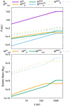 |
Fig. 1. Top panel: radius of bubbles outside the jet (yellow), right after penetrating the jet (green) and at stagnation (blue) compared to the radius of the jet, as a function of jet height. Bottom panel: mass within bubbles of radius Rout (yellow), and Rin (green), as a function of jet height. Parameters used are Lj = 1044 erg s−1, Γj = 10 and the orbital values given in Sect. 2.2. Values for both a red giant of average mass-loss rate (solid line) and a red giant that generates the dominant events (dashed line, see Sect. 5.2) are plotted. |
For the particular set of parameters used to plot Fig. 1, above z ∼ 400 pc the size of the bubble inside the jet is shown as larger than the size of the bubble outside the jet. In such a case, the material introduced into the jet would be that contained within Rs − Rout. Another possibility, for a different set of parameters, is that Rs is larger than Rin, but smaller than Rout. In such a case, the star would lose any outer layers in the CD, and once inside the jet, the stellar wind termination region would expand up to the stagnation radius.
Figure 1 shows the mass contained in the bubble outside and right after penetrating the jet, for the average and the event-dominant mass-loss rates. The jet is loaded with the external matter brought by the bubbles expelled by stars at penetration, though this mass-load rate is much lower than the jet Ṁjet = Lj/Γjc2, and therefore unlikely to result in a dynamical effect on the jet.
As has been studied for example by Wykes et al. (2015) and Vieyro et al. (2017), a population of high-mass stars in starburst galaxies can interact strongly with the jet. Young OB stars have stronger winds than red giants, with higher mass-loss rates and speeds. However, these stars have such fast winds that vw > vorb. Following Eq. (5), when that condition is met, Rs > Rin. Therefore, the star penetrates the jet and the size of the interaction region surrounding the star actually increases, with no significant external material introduced into the jet.
4. Bubble evolution within the jet
We consider a jet that initially expands with a conical geometry, launched close to the supermassive black hole in the centre of the galaxy. We consider that the jet recollimates, which we model as the jet becoming cylindrical:
 (7)
(7)
when its pressure becomes equal to that of the ISM.
After the star penetrates the jet and a bubble of stellar material is expelled, this bubble evolves as a result of the interaction with the jet. We have adopted the analytical modelling of the evolution of a blob impacted by a jet developed by Barkov et al. (2010, 2012) and Khangulyan et al. (2013; for previous numerical simulations of this process, see e.g. Bosch-Ramon et al. 2012; Perucho et al. 2017).
The shock produced by the impact of the jet ram pressure causes the material of the bubble to heat up, quickly expand, and accelerate, resulting in the bubble reaching relativistic speeds. This acceleration occurs on timescales of
 (8)
(8)
where D is a dimensionless parameter related to the jet luminosity and Lorentz factor and the mass of the bubble, Rb is the radius of the bubble after acceleration (see e.g. Barkov et al. 2012), and any subindex “0” refers to the value at z0, the height at which the star penetrates. The value D actually gives a comparison between bubble and jet mass on scales of z0; that is, if D > 1 (< 1), the jet will (not) effectively accelerate the blob before it covers a distance ∼z0. After the blob is accelerated, it is carried downstream (likely at least partially disrupted) until jet termination, at a height H and at a speed ∼βc, thus on a timescale tesc ∼ (H − z0)/βc.
This analytical approximation to the bubble evolution within the jet, which we use to calculate the results presented in Sect. 5, can be compared to results obtained through numerical simulations. For that, we simulate here the bubble-jet interaction solving numerically the equations of relativistic hydrodynamics (RHD) assuming axisymmetry, a gas with constant adiabatic index  , and a dynamically negligible magnetic field. The RHD equations are solved using the Marquina flux formula (Donat & Marquina 1996; Donat et al. 1998); further details on the code can be found in de la Cita et al. (2016).
The resolution of the calculations is 1000 cells in the vertical direction, the z-axis, and 200 in the radial direction, the r-axis. Those numbers of cells correspond to a physical range of zgrid = 1000 − 1300 pc and rgrid = 0 − 65 pc. The number of cells was chosen such that the results did not change significantly when going to higher resolution. The boundary conditions were set to inflow at zgrid = 0 with parallel stream lines (the jet is recollimated), reflection at rgrid = 0, and outflow in the remaining boundaries.
Figure 2 shows three density maps, illustrative snapshots of a simulation of the jet-bubble interaction at ∼0.4, 400, and 950 yr after bubble penetration inside the jet. Initial properties are: Lj = 1044 erg s−1, Γj = 10, Mb = 2 × 10⁻⁶ M⊙, and rb, 0 = 1.5 pc. The simulation starts once the cloud has already expanded significantly, moving with a Lorentz factor of 2, in the relativistic regime (e.g. Barkov et al. 2012; Khangulyan et al. 2013). We focus only on the relativistic regime, as starting from its actual initial radius would require 102 − 1002 times more cells and thus huge computing costs. As seen in the figure, the shocked bubble evolves upstream of the jet; most of the bubble expansion occurs at early times, and despite partial disruption the structure keeps its integrity.
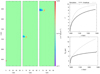 |
Fig. 2. Left panel: density maps obtained from a hydrodynamic simulation of the interaction between the jet and the penetrating bubble. Three snapshots are taken ∼0.4, 400 and 950 yr after penetration to illustrate bubble evolution. Right panels: bubble Lorentz factor/bubble radius as a function of jet height as calculated through the analytical estimate (dotted line) of Barkov et al. (2010, 2012), used to derive all results presented in this work, and compared to those obtained through our simulations (solid line). |
In Fig. 2 we also plot the bubble radius and Lorentz factor as a function of jet height obtained from the simulation, and compare it to the results of the analytical calculation. The simulated evolution is slightly slower than analytically predicted. We note, however, that while the Lorentz factor of the bubble in the simulation reaches a value of ∼8, it should eventually reach the jet Lorentz factor at higher z. The chosen duration of the simulation of ∼1000 yr was adopted as a trade-off between a moderated computational time and illustrative effectiveness.
A noticeable difference in Fig. 2 between simulated and analytical results is bubble radius, computed as the mass-averaged cylindrical radius to facilitate comparison. The radius evolves more slowly in the simulation, reaching a final value of a factor ≲2 smaller than the analytical estimate. We expect nevertheless more convergence at larger z values.
We show thus that the analytical first-order approximation to the bubble evolution used in this work, adopted to derive the results presented in Table 1, is reasonably accurate in the relativistic regime. While instabilities might be important, once the shocked bubble reaches relativistic speeds, its evolution is similar to the analytic predictions, even if disrupted as a filamentary fragmented structure mixed with shocked jet material. The reason is that the transversal expansion of the shocked bubble material is slowed down in the laboratory frame by flow-frame time dilation, and in the longitudinal direction by very similar bottom and the top speeds of the shocked structure in the laboratory frame.
Results.
Therefore, from the simulation results, we find it reasonable at this stage to adopt a final constant bubble radius, and a final bubble speed close to that of the jet if D > 1. For the bubbles that dominate the non-thermal emission (see Sect. 5.2), this condition is fulfilled.
A more complete simulation, including earlier and later stages of the bubble evolution, is planned for future work.
5. Radiated non-thermal power
Particles are assumed to be efficiently accelerated at the interaction between the jet and the bubble. The non-thermal energy contained in these particles is uncertain, although we focus here on the case in which the energy budget is significant and detectable radiation may be produced. The specific acceleration mechanism is not considered, and it is just assumed that some fraction of the shocked jet luminosity goes to non-thermal particles.
5.1. Energy losses
We assume that electrons (and positrons) are the dominant non-thermal emitting particles. Accelerated protons may also be present in the jet, although on the scales of interest significant radiation losses are not expected for these particles (see however, e.g. Aharonian 2000). For electrons, we considered the radiative losses via inverse Compton (IC) and synchrotron emission. Regarding non-radiative losses, we considered adiabatic losses for the conical jet, and none after recollimation (but escape when the bubble reaches H).
We computed the IC losses as in Bosch-Ramon & Khangulyan (2009; see also Khangulyan et al. 2014). Their approximation is valid for a Planck distribution of target photons of temperature T, and must be renormalized to the energy density of the considered target photon field. We consider the photon field in an elliptical galaxy as derived by Vieyro et al. (2017).
We also considered synchrotron losses (e.g. Longair 1981) when taking B = Beq, a magnetic field of equivalent energy density to that of the jet, meaning
 (9)
(9)
with the field depending on height as
 (10)
(10)
where B0 = B(z0). We discuss the effects on the synchrotron radiation of considering a lower magnetic field in Sect. 5.2.3.
5.2. Radiation
For all combinations of Lj = 1043, 1044, 1045, and Γj = 3, 10, we computed the average luminosity of the whole population of bubbles penetrating the jet (as seen by the observer), Lpop. Results are presented in Table 1. All parameters except for jet luminosity, Lj, and Lorentz factor, Γj, are fixed as described in Sects. 2 and 3.
We evaluated the emitted non-thermal radiation at two characteristic electron energies: first, for IC emission, at the Thompson-Klein Nishina transition energy, at  , where the maximum of IC emission is expected for reasonable electron energy distributions, falling in the gigaelectronvolt-Teraelectronvolt range; secondly, for synchrotron emission, for the electrons that generate synchrotron 100 MeV photons as seen by the observer, at
  .
.
We assumed that at most a fraction η of the energy acquired by jet acceleration can be radiated2, fixed to 0.1 throughout this work. From first principles, it is not possible to derive the value of η, but the adopted choice maximizes the predicted gamma-ray emission without assuming a full non-thermal conversion of the available energy. All the predicted luminosities thus scale with η/0.1 ≤ 10.
We estimated the typical properties of the bubbles that contribute the most to the overall luminosity as
 (11)
(11)
where A denotes the quantity we are interested in evaluating (i.e. Mb and z0). We refer to events with these properties as the “dominant” events, and list their characteristics in Table 1. Their penetration rate (i.e. rate at which events occur) along with peak luminosity of the event, Ldom or Lpeak, and typical duration of the peak, tobs or tpeak, are also listed. We note that Ldom is the average luminosity of a dominant event along its evolution within the jet; in reality, the luminosity is a function of jet height (see Eq. (13)), larger at z0, where the star penetrates, and becomes progressively dimmer as the radiative cooling efficiency diminishes.
We also compared the emission generated through this interaction mechanism to that generated in steady state, Lst, by the same population of red giants (see Sect. 3). The apparent non-thermal luminosity per unit volume at a height z due to jet-star interactions in steady state is
 (12)
(12)
where ⟨Ss(m, t)/Sj⟩ is the time-averaged fraction of jet area intercepted by one stellar interaction.
5.2.1. Inverse Compton emission
At electron energies  , for all jet parameters considered,
  s. This is much larger than the characteristic acceleration time of any considered bubble, typically in the range
  s. Therefore, the IC emission at the energy of interest will last until long after the bubble has been accelerated.
As the bubble propagates downstream in the jet, the former radiates an IC luminosity  in the flow frame, where
  is the total energy emitted by one single bubble in the same frame during its evolution
 (13)
(13)
zmax is the maximum height the bubble reaches before losing all energy, or the jet maximum height, H. This approximation implicitly assumes that the energy distribution of the non-thermal electrons is ∝E−2 (see Sect. 6.2).
Characteristic times for energy losses evaluated at  , as well as
  , are plotted in Fig. 3. The energy losses are dominated by adiabatic expansion up to the jet recollimation point. At higher z, the shortest timescale is
  , meaning the bubbles exit the jet before emitting (mostly through IC) all of their available energy.
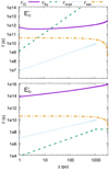 |
Fig. 3. Inverse Compton and synchrotron loss times for a jet with Lj = 1044 erg s−1, Γj = 10, and (top panel) B = 0.1Beq, evaluated at |


We note that, contrary to the study of synchrotron gamma-ray emission below, IC energy losses are computed taking B = 0.1Beq, which is a reasonable value for a jet with power dominated by its kinetic energy. However, since the energy losses at  are dominated by non-radiative processes, considering more (or less) intense magnetic fields does not significantly affect the results.
We can estimate the luminosity detected by an observer, generated by the whole bubble population, averaged in time as
 (14)
(14)
where δj is the Doppler boosting factor. This is a valid description as long as there is more than one dominant bubble simultaneously emitting3, meaning that the source duty cycle is larger than 1. In addition, the emission generated by the whole population, Lpop, as seen by the observer will be larger than the emission produced by one single, dominant event, Ldom.
The predicted apparent luminosities of the IC emission are a few times 1040 erg s−1. These values are of the order of the steady state emission generated by the whole stellar population within the jet.
5.2.2. Synchrotron emission
If we evaluate the energy losses at  ,
,  is dominant at all heights for
  (see Fig. 3). The synchrotron emission is so intense that the characteristic emission time is lower than the acceleration time of the bubble,
  . Therefore, electrons of energy
  immediately radiate via synchrotron emission the energy acquired via particle acceleration triggered by the jet-bubble interaction. Electrons in the flow frame are accelerated at a rate ξqB′c, where ξ, a free parameter representing the acceleration efficiency, is fixed to 0.1. Such an efficiency is sufficient to produce observable 100 MeV synchrotron photons, although for ξ well below 0.1 synchrotron emission would not reach gamma-ray energies (X-rays of luminosities similar to those of IC in Table 1 could still be produced).
Synchrotron 100 MeV photons are produced when a single bubble enters the jet and is accelerated, following a flare-like lightcurve (see Barkov et al. 2012). From Khangulyan et al. (2013), the apparent total energy emitted by a bubble in the synchrotron fast cooling regime is:
 (15)
(15)
where we take  (Barkov et al. 2010), and Frad is the efficiency with which the particle loses energy through synchrotron radiation. Doppler boosting is already accounted for in Eq. (15) for the energy radiated by one single bubble.
Unlike in the case of the IC emission, synchrotron Lpeak is 1–3 orders of magnitude higher than the average luminosity Lpop, with
 (16)
(16)
where we take Fe, max = 0.4 (Barkov et al. 2010), and rb is the radius of the bubble once it has expanded and reached relativistic velocities (Khangulyan et al. 2013). The apparent duration of this intense emission can be roughly estimated as tpeak = Eb/Lb, which shows that the emission is highly variable, like intense, short flares occurring a few times per century or millennia.
For the high ξ adopted, the synchrotron 100 MeV emission could reach luminosities of ∼1044 erg s−1 for the most powerful jets considered, even under low jet Lorentz factors. As the emission is intense but short, we would have duty cycles of PR ⋅ tobs ∼ 10−4 − 10−2, depending on Lj and Γj.
5.2.3. Synchrotron emission at low magnetic fields
Synchrotron emission at ∼100 MeV is highly dependent on the value of the magnetic field: high magnetic fields yield an intense emission radiated in a very short amount of time, yielding a low duty cycle.
In order to maximize the duty cycle, we take the lowest possible value of the magnetic field, B = Bmin, for which electrons with  still cool more efficiently through synchrotron emission than through non-radiative losses. Looking at Fig. 3, this would result in values of
  just below
  and/or
  . The obtained magnetic field values, Bmin, are listed in Table 1. For these values of B, luminosity is up to ∼1042 erg s−1, but the duty cycle can be increased up to PR ⋅ tobs > 1.
We note that in this case with B = Bmin,  , meaning that the synchrotron emission is computed as described in Sect. 5.2.1, that is, as is done for inverse Compton radiation.
6. Discussion
The dynamical evolution of a bubble of stellar material expelled within the jet is semi-quantitatively well-described by the analytical estimates used in Sect. 4, and only differs from simulations by a moderate numerical factor. Our numerical estimates on gamma-ray energy production are not significantly affected by these differences as long as the bubble Lorentz factor eventually reaches ∼Γj. Only in the case of intense Synchrotron emission at high magnetic fields, could there be a small reduction of luminosity, of a factor of a few, if indeed the bubble radius were overestimated in the long run.
Results presented in Table 1 indicate that the emission generated by stars penetrating the jet can be relatively persistent at high energies, through either inverse Compton or through synchrotron emission in the case of low magnetic fields. With large magnetic fields, emission at 100 MeV could be dominated by bright and infrequent events on top of the persistent, lower IC radiation.
The steady state emission of the whole population is unlikely to be detectable. We note that the similar values of Lst for all the explored jet configurations are due to the fact that it does not strongly depend on either Γj or Lj. The small differences are due to jet geometry, which influences the amount of stars within the jet (e.g. a jet of Lj = 1043 erg s−1 recollimates at low heights), or due to differences in Frad (e.g. under high B values, for Lj = 1045 the impact of synchrotron losses on electrons at  is noticeable).
Inverse Compton emission of the bubbles at  seems difficult to detect for the explored jet configurations unless η → 1, or for a very nearby source. This is because non-radiative losses, or even synchrotron losses, dominate the process.
Synchrotron emission at  with high magnetic fields can result in bright, detectable flares, although the high luminosity implies a short duration. If we consider lower magnetic fields, persistent emission can be achieved, and luminosities of the order of 1042 erg s−1 for Γj = 10.
There are some factors that may easily increase the radiation in the scenario studied here. For instance, for significantly lower values of ρISM at z∼ kpc, say ≳0.1 cm−3, the emission energetics would grow by a factor of several due to the associated larger bubble mass (see Sect. 3.2), limited now by Min (see Fig. 1). Furthermore, a younger, more massive red giant population, or the sporadic presence of an asymptotic giant branch (AGB) star within the jet, could also enhance the expected emission.
6.1. Younger red giant populations and AGB stars
Our results show that the emission produced by wind bubbles as they penetrate the jet is generally dominated by the most evolved stars within our modelled population (with Ṁ ∼ 1.4 × 10⁻⁸M⊙ yr−1). The mass of the bubbles scales with mass-loss rate as ∝ Ṁ3/2, and the luminosity emitted by the bubble interacting with the jet is proportional to its mass (except for the case of synchrotron emission of 100 MeV photons at Beq). Therefore, our results are scalable with mass-loss rate.
If we had a population of red giants of MRG = 1.5 M⊙ with a total mass comparable to that of the Galaxy, it would imply an increase of luminosity of a factor of ∼20 in the case of low-B synchrotron emission, and of a factor of ∼60 in the case of Inverse Compton emission. In the case of high-B emission, emission depends on the final radius of the bubble, and it would increase by a factor of ∼6. In all cases, considering these less abundant stars would lead to a decrease of event occurences of ∼0.4.
We note that in the rare occasion an AGB star penetrates an AGN jet, its wind bubble can inject into the latter up to ∼10−2 M⊙. This could potentially lead to a long duration event with IC luminosity ∼1044 erg s−1.
6.2. Caveats of the radiation estimates
In this work we estimate the energy radiated by accelerated particles at a given energy,  , where the maximum of emission is expected to be. In assuming that all the available energy that goes into particle acceleration is radiated or lost at the mentioned energy, we are overestimating the overall emission. Depending on the energy distribution of the particles, this simple approximation can differ from a more precise calculation. In the case of inverse Compton emission, we expect this overestimation to be of a factor of a few, and in the case of synchrotron emission, of up to one order of magnitude (Vieyro et al. 2017, and in prep.). This has to be taken into account when reading the luminosities in Table 1. The approximations adopted are valid for electron energy distributions ∝E2, typical for astrophysical sources. Harder electron distributions would still lead to similar results to those obtained but for very extreme cases, while steeper distributions would imply an even higher overestimate of the gamma-ray luminosity.
The radiation estimates were focused on gamma rays and a broad band study would require more detailed modelling. Nevertheless, it is worth exploring in the future the radio and X-ray synchrotron emission in the jet-bubble interactions.
7. Summary
In this work we have studied the gamma-ray emission produced when the bubbles formed by red giant winds penetrate the jet of a blazar in an elliptical galaxy, and described their dynamical evolution both analytically and through one illustrative simulation. We have shown that the analytical approximation is reasonably accurate at the present stage in the relativistic regime. We have found that the gamma rays produced by the red giant wind bubbles interacting with jets may reach detectable levels if Lorentz factors are high, non-thermal particles are generated very efficiently, and particle acceleration takes place at very high rates (to produce synchrotron 100 MeV photons). This predicted emission could be higher under the presence of an important population of younger red giants, in the rare event an AGB star enters the jet, or for relatively low values of ρISM. Unless B = Beq, duty cycles are not far below one, and in some cases, a few dominant bubbles could contribute simultaneously to the gamma-ray emission. For B = Beq, short bright synchrotron 100 MeV flares may be detected, with year or sub-year scale duration. Most of the known blazars in the local universe are hosted by elliptical galaxies. Therefore, provided that electrons are efficiently accelerated in bubble-jet interactions, it is plausible that some persistent or transient gamma-ray emission detected from the nearest blazars could originate in events like those described here.
Instabilities produced at the jet-wind interaction region may actually lead to individual star-jet interaction variability (de la Cita et al. 2016).
The bubble acquires in the laboratory frame an energy ∼ΓjMbc2 due to jet acceleration.
The Doppler-boosted luminosity of one single bubble is  . If more than one star is within the jet emitting at different heights, the photons emitted by the distribution of sources at the same time in K′ are not observed simultaneously in K, leading to δ4 → δ3/Γ (see Sikora et al. 1997). Thus, if insufficient events take place at the same time, the apparent luminosity of the whole population can be reduced to that of one single bubble.
Acknowledgments
We want to thank the anonymous referee for constructive and useful comments. We acknowledge support by the Spanish Ministerio de Economía y Competitividad (MINECO/FEDER, UE) under grants AYA2013-47447-C3-1-P, AYA2016-76012-C3-1-P, with partial support by the European Regional Development Fund (ERDF/FEDER), MDM-2014-0369 of ICCUB (Unidad de Excelencia “María de Maeztu”), and the Catalan DEC grant 2017 SGR 643. N.T-A. acknowledges support from MINECO through FPU14/04887 grant.
References
- Aharonian, F. A. 2000, New Astron., 5, 377 [NASA ADS] [CrossRef] [Google Scholar]
- Araudo, A. T., Bosch-Ramon, V., & Romero, G. E. 2013, MNRAS, 436, 3626 [NASA ADS] [CrossRef] [Google Scholar]
- Barkov, M. V., Aharonian, F. A., & Bosch-Ramon, V. 2010, ApJ, 724, 1517 [NASA ADS] [CrossRef] [Google Scholar]
- Barkov, M. V., Aharonian, F. A., Bogovalov, S. V., Kelner, S. R., & Khangulyan, D. 2012, ApJ, 749, 119 [NASA ADS] [CrossRef] [Google Scholar]
- Bednarek, W., & Banasiński, P. 2015, ApJ, 807, 168 [NASA ADS] [CrossRef] [Google Scholar]
- Bednarek, W., & Protheroe, R. J. 1997, MNRAS, 287, L9 [NASA ADS] [CrossRef] [Google Scholar]
- Begelman, M. C., Blandford, R. D., & Rees, M. J. 1984, Rev. Mod. Phys., 56, 255 [NASA ADS] [CrossRef] [Google Scholar]
- Blandford, R. D., & Koenigl, A. 1979, Astrophys. Lett., 20, 15 [NASA ADS] [Google Scholar]
- Bosch-Ramon, V. 2015, A&A, 575, A109 [NASA ADS] [CrossRef] [EDP Sciences] [Google Scholar]
- Bosch-Ramon, V., & Barkov, M. V. 2016, A&A, 590, A119 [NASA ADS] [CrossRef] [EDP Sciences] [Google Scholar]
- Bosch-Ramon, V., & Khangulyan, D. 2009, Int. J. Mod. Phys. D, 18, 347 [NASA ADS] [CrossRef] [Google Scholar]
- Bosch-Ramon, V., Perucho, M., & Barkov, M. V. 2012, A&A, 539, A69 [NASA ADS] [CrossRef] [EDP Sciences] [Google Scholar]
- Bowman, M., Leahy, J. P., & Komissarov, S. S. 1996, MNRAS, 279, 899 [NASA ADS] [CrossRef] [Google Scholar]
- Crowley, C. 2006, PhD Thesis, School of Physics, Trinity College Dublin, Dublin 2, Ireland [Google Scholar]
- de la Cita, V. M., Bosch-Ramon, V., Paredes-Fortuny, X., Khangulyan, D., & Perucho, M. 2016, A&A, 591, A15 [NASA ADS] [CrossRef] [EDP Sciences] [Google Scholar]
- Donat, R., & Marquina, A. 1996, J. Comput. Phys., 125, 42 [NASA ADS] [CrossRef] [Google Scholar]
- Donat, R., Font, J. A., Ibáñez, J. M. l., & Marquina, A. 1998, J. Comput. Phys., 146, 58 [NASA ADS] [CrossRef] [Google Scholar]
- Espey, B. R., & Crowley, C. 2008, ASP Conf. Ser., 401, 166 [NASA ADS] [Google Scholar]
- Falomo, R., Pian, E., & Treves, A. 2014, A&ARv, 22, 73 [NASA ADS] [CrossRef] [Google Scholar]
- Gebhardt, K., & Thomas, J. 2009, ApJ, 700, 1690 [NASA ADS] [CrossRef] [Google Scholar]
- Gebhardt, K., Adams, J., Richstone, D., et al. 2011, ApJ, 729, 119 [NASA ADS] [CrossRef] [Google Scholar]
- Harris, D. E., Biretta, J. A., & Junor, W. 1999, Lect. Notes Phys., 530, 100 [NASA ADS] [CrossRef] [Google Scholar]
- Hubbard, A., & Blackman, E. G. 2006, MNRAS, 371, 1717 [NASA ADS] [CrossRef] [Google Scholar]
- Khangulyan, D. V., Barkov, M. V., Bosch-Ramon, V., Aharonian, F. A., & Dorodnitsyn, A. V. 2013, ApJ, 774, 113 [NASA ADS] [CrossRef] [Google Scholar]
- Khangulyan, D., Aharonian, F. A., & Kelner, S. R. 2014, ApJ, 783, 100 [NASA ADS] [CrossRef] [Google Scholar]
- Komissarov, S. S. 1994, MNRAS, 269, 394 [NASA ADS] [CrossRef] [Google Scholar]
- Kroupa, P. 2001, MNRAS, 322, 231 [NASA ADS] [CrossRef] [Google Scholar]
- Longair, M. S. 1981, High Energy Astrophysics (Cambridge and New York: Cambridge University Press) [Google Scholar]
- Nilsson, K., Pursimo, T., Heidt, J., et al. 2003, A&A, 400, 95 [NASA ADS] [CrossRef] [EDP Sciences] [Google Scholar]
- Olguín-Iglesias, A., León-Tavares, J., Kotilainen, J. K., et al. 2016, MNRAS, 460, 3202 [NASA ADS] [CrossRef] [Google Scholar]
- Perucho, M., Martí, J. M., Laing, R. A., & Hardee, P. E. 2014, MNRAS, 441, 1488 [NASA ADS] [CrossRef] [Google Scholar]
- Perucho, M., Bosch-Ramon, V., & Barkov, M. V. 2017, A&A, 606, A40 [NASA ADS] [CrossRef] [EDP Sciences] [Google Scholar]
- Reimers, D. 1975, Mem. Soc. R. Sci. Liege, 8, 369 [NASA ADS] [Google Scholar]
- Scarpa, R., Urry, C. M., Padovani, P., Calzetti, D., & O’Dowd, M. 2000, ApJ, 544, 258 [NASA ADS] [CrossRef] [Google Scholar]
- Sikora, M., Madejski, G., Moderski, R., & Poutanen, J. 1997, ApJ, 484, 108 [NASA ADS] [CrossRef] [Google Scholar]
- Sutherland, R. S., & Bicknell, G. V. 2007, ApJS, 173, 37 [NASA ADS] [CrossRef] [Google Scholar]
- Tan, J. C., Beuther, H., Walter, F., & Blackman, E. G. 2008, ApJ, 689, 775 [NASA ADS] [CrossRef] [Google Scholar]
- Vieyro, F. L., Torres-Albà, N., & Bosch-Ramon, V. 2017, A&A, 604, A57 [NASA ADS] [CrossRef] [EDP Sciences] [Google Scholar]
- Wang, Z., Wiita, P. J., & Hooda, J. S. 2000, ApJ, 534, 201 [NASA ADS] [CrossRef] [Google Scholar]
- Wykes, S., Hardcastle, M. J., Karakas, A. I., & Vink, J. S. 2015, MNRAS, 447, 1001 [NASA ADS] [CrossRef] [Google Scholar]
All Tables
All Figures
|
Fig. 1. Top panel: radius of bubbles outside the jet (yellow), right after penetrating the jet (green) and at stagnation (blue) compared to the radius of the jet, as a function of jet height. Bottom panel: mass within bubbles of radius Rout (yellow), and Rin (green), as a function of jet height. Parameters used are Lj = 1044 erg s−1, Γj = 10 and the orbital values given in Sect. 2.2. Values for both a red giant of average mass-loss rate (solid line) and a red giant that generates the dominant events (dashed line, see Sect. 5.2) are plotted. |
| In the text | |
|
Fig. 2. Left panel: density maps obtained from a hydrodynamic simulation of the interaction between the jet and the penetrating bubble. Three snapshots are taken ∼0.4, 400 and 950 yr after penetration to illustrate bubble evolution. Right panels: bubble Lorentz factor/bubble radius as a function of jet height as calculated through the analytical estimate (dotted line) of Barkov et al. (2010, 2012), used to derive all results presented in this work, and compared to those obtained through our simulations (solid line). |
| In the text | |
|
Fig. 3. Inverse Compton and synchrotron loss times for a jet with Lj = 1044 erg s−1, Γj = 10, and (top panel) B = 0.1Beq, evaluated at |
| In the text | |
Current usage metrics show cumulative count of Article Views (full-text article views including HTML views, PDF and ePub downloads, according to the available data) and Abstracts Views on Vision4Press platform.
Data correspond to usage on the plateform after 2015. The current usage metrics is available 48-96 hours after online publication and is updated daily on week days.
Initial download of the metrics may take a while.