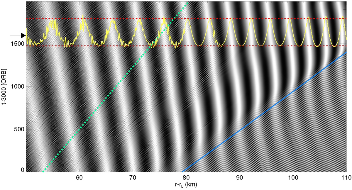
Stroboscopic space–time diagram of a 60 km section of τ resulting from the same hydrodynamical integration using β = 1.20 and scaled torque as displayed in Fig. C.1 for times t = 3000–5000 ORB. The over-plotted τ-profile describes the state at time t = 1600 ORB and the red dashed lines indicate the maximum and minimum values of τ predicted by Eq. (35) for q = 0.25. The blue solid line describes the expected location of the density wavefront based on the group velocity (Eq. (42)). Overstable waves at radial distances r– r_L ≳ 90 km are fully damped once the density wavefront has passed this region. At considerably larger radial distances where the density wave has damped substantially, overstability reappears (see Fig. C.1, fourth row). The green dashed line indicates the nonlinear phase velocity ω_I ∕k of overstablewaves with λ = 250 m (Fig. 8). Overstable waves existing at distances r–r_L ~ 80 − 110 km before the density wavefront arrives possess small amplitude perturbations (the slowly left traveling narrow features). These are expected to propagate with the nonlinear group velocity d ω_I ∕d k of the overstable waves (Latter & Ogilvie 2010; LSS2017), which is small since the wavelength λ of the wavesis close to the (nonlinear) frequency minimum (Fig. 8).