| Issue |
A&A
Volume 622, February 2019
|
|
|---|---|---|
| Article Number | L5 | |
| Number of page(s) | 6 | |
| Section | Letters to the Editor | |
| DOI | https://doi.org/10.1051/0004-6361/201834806 | |
| Published online | 29 January 2019 | |
Letter to the Editor
Shape evolution of cometary nuclei via anisotropic mass loss
1
Institute of Applied Astronomy of the Russian Academy of Sciences, St. Petersburg, Russia
e-mail: This email address is being protected from spambots. You need JavaScript enabled to view it.
2
Department of Astronomy, University of Washington, Seattle, WA, USA
e-mail: This email address is being protected from spambots. You need JavaScript enabled to view it.
3
Chebyshev Laboratory, St. Petersburg State University, St. Petersburg, Russia
4
St. Petersburg Department of V.A. Steklov Institute of Mathematics of the Russian Academy of Sciences, St. Petersburg, Russia
Received:
10
December
2018
Accepted:
26
December
2018
Abstract
Context. Breathtaking imagery recorded during the European Space Agency Rosetta mission confirmed the bilobate nature of the nucleus of comet 67P/Churyumov-Gerasimenko. The peculiar appearance of the nucleus is not unique among comets. The majority of cometary cores imaged at high resolution exhibit a similar build. Various theories have been brought forward as to how cometary nuclei attain such peculiar shapes.
Aims. We illustrate that anisotropic mass loss and local collapse of subsurface structures caused by non-uniform exposure of the nucleus to solar irradiation can transform initially spherical comet cores into bilobed cores.
Methods. We derived a mathematical framework to describe the changes in morphology resulting from non-uniform insolation during the spin-orbit evolution of a nucleus. We solved the resulting partial differential equations that govern the change in the shape of a nucleus subject to mass loss and consequent collapse of depleted subsurface structures analytically for simple insolation configurations and numerically for more realistic scenarios.
Results. The proposed mechanism is capable of explaining why a large percentage of periodic comets appear to have peanut-shaped cores and why light-curve amplitudes of comet nuclei are on average larger than those of typical main belt asteroids of the same size.
Key words: comets: general / comets: individual: 67P/Churumov-Gerasimenko
© ESO 2019
1. Introduction
Bilobed configurations appear to be common in cometary nuclei. The detailed imagery recorded in the framework of the Rosetta mission saw 67P/Churyumov-Gerasimenko (67P) join the ranks of dumbbell-shaped comets alongside 103P/Hartley 2, 19P/Borrelly, 1P/Halley, and 8P/Tuttle (Keller et al. 2015; Massironi et al. 2015; Davidsson et al. 2016), as shown in Fig. 1. Current hypotheses as to how such peculiar shapes emerge range from high speed collisions of proto-comets (Jutzi et al. 2017; Jutzi & Benz 2017; Brunini 2017) over fission and reconfiguration (Schwartz et al. 2018; Hirabayashi et al. 2016) to a slow merging of two separately formed proto-cores on similar orbits (Jutzi & Asphaug 2015). Apart from collisions, gradual mass loss through sublimation has long been considered a possible mechanism to shape cometary nuclei (Jewitt et al. 2003). The surface of 67P, for instance, shows significant outgassing and changes to its surface when exposed to solar radiation (Sierks et al. 2015). The corresponding loss of water-ice mixed with other chemical compounds can be substantial for short period comets that approach the Sun on a regular basis. The surface thickness of 67P, for instance, is believed to shrink on average by 1.0 ± 0.5 m per orbit (Bertaux 2015). Exposure to sunlight can vary over the surface of a comet depending on its geometry and spin state (Sierks et al. 2015). How small differences in local insolation, sublimation, and outgassing rates sculpt cometary nuclei over their lifetime is one of the key concerns of this work.
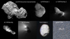 |
Fig. 1. Cometary nuclei imaged from spacecraft encounters or ground-based radar. Panel a: 67P/Churyumov-Gerasimenko. Image credit: ESA/Rosetta/MPS for OSIRIS Team MPS/UPD/LAM/IAA/SSO/ INTA/UPM/DASP/IDA. Panel b: 9P/Tempel 1. Image credit: PIA02142, Courtesy NASA/JPL-Caltech. Panel c: 103P/Hartley 2. Image credit: PIA13570, Courtesy NASA/JPL-Caltech. Panel d: 19P/Borelly. Image credit: PIA03500, Courtesy NASA/JPL-Caltech. Panel e: 1P/Halley. Image credit: ESA/MPS. Panel f: 81P/Wild 2, see Duxbury et al. (2004). Panel g: 8P/Tuttle. Image credit: Arecibo Observatory Planetary Radar, resolution 1 μs × 0.5 Hz, see Harmon et al. (2010). |
Comets are believed to form in the outer solar system as kilometre-sized, single-lobed objects (Davidsson et al. 2016). On the journey towards the inner solar system the outer shell of a cometary nucleus is dehydrated and accumulates coatings rich in organic compounds on top of a layer of ice (Filacchione et al. 2016; Fornasier et al. 2016). The nucleus is also heated periodically by incident sunlight subject to the rotation of the core. As a consequence of periodic heating, the subsurface layers of the nucleus experience depletion of cryomagma and consequent structural collapse leading to a localized compactification of core material (Miles 2016). Even if a newly formed cometary core was largely homogenous to begin with, the afore mentioned processes would foster radial disparity in the core of the nucleus. The denser, outer shell depleted of volatiles is less likely to allow cometary material to be lost at elevated rates. The material closer to the core retains a high volatile content and a relatively low bulk density.
Should the nucleus lose some of its shell the local differences in mass loss rates could change the shape of the core of the comet in a non-trivial fashion. Subsurface material could be exposed, for instance, as a consequence of non-catastrophic collisions (Schwartz et al. 2018). Collision probabilities for comets in the outer solar system are hard to quantify, however. In this work, we, thus, focus on the more general concept of anisotropic mass loss.
2. Carving cometary nuclei through anisotropic mass loss
For comets in principle axis rotation the energy input from the sun is highest around the subsolar manifold of the nucleus, which is the path on the surface of the nucleus that experiences the largest insolation over one spin period. Since the penetration depth of the sublimation front into the core is proportional to the local energy input, mass loss rates in those regions are enhanced compared to the rest of the core. Nuclei with spin axis orientations perpendicular to their orbital plane, for instance, are bound to lose matter more quickly around their “waist” (Fig. 2). The collapse of desiccated subsurface structures and formation of sinkholes can bring the new surface layer closer to more pristine material in the centre of the core (Miles 2016). The now volatile rich subsurface once again yields higher mass loss rates. Over time, this process of anisotropic mass loss can reshape the nucleus of a comet into a more elongated form.
 |
Fig. 2. Shape and spin evolution of cometary nuclei can lead to bilobed shapes. |
The more elongated affected cometary cores become, however, the more the principle moment of inertia decreases around the primary axis of rotation of the nucleus. Torques induced by localized outgassing such as jets or close encounters with planets can then destabilize the spin axis leading to the complex rotation states observed in the majority of comets. Mass loss continues to alter the shape of the comet even in complex rotation states. Our simulations show that if the distance of a comet to the sun remains large enough to avoid disintegration within a few orbits, a wide variety of geometries of cometary nuclei arise naturally (Fig. 3). How quickly anisotropic mass loss changes the shape of a comet depends on the size and spin-orbit evolution of the comet (see Appendix B).
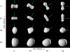 |
Fig. 3. Possible shapes of cometary nuclei as a result of anisotropic mass loss are shown for a variety of configurations. The outcome is determined by the initial obliquity of the nucleus before substantial mass loss sets in (α1) and final obliquity after destabilization of the original spin state (α2). The corresponding spin axes are red and green, respectively. The nuclei in this graph are orientated according to their final obliquity with respect to the orbital angular momentum (vertical direction). |
Forming bilobate shapes such as those of 67P through the proposed mechanism requires the rate of mass loss in the outer shell of the cometary core to be smaller than that that closer to the interior of the primordial body. Otherwise, if the mass loss rate is homogeneous or decreases towards the centre of the core, the shape of the shape remains convex. Given the processing and desiccation the outer shell experiences over the lifetime of a comet, in particular before the latter enters the inner solar system, precisely such a configuration would be expected (Miles 2016). Mass loss rates of material closer to the core remain high due to the higher volatile content. If 67P formed as a single, roughly spherical object, the so-called neck (Hapi) region would have been close to the primordial core, and Hapi shows enhanced outgassing activity compared to other domains on 67P (Sierks et al. 2015). We would like to stress that the higher outgassing rates near Hapi were not caused by enhanced insolation at the time of observation. In fact, the neck received around 15% less sunlight than other regions (Sierks et al. 2015). Higher mass loss rates around the neck, thus, point towards compositional or structural differences compared to the rest of the comet, which is in line with our model.
One of the main arguments against 67P being an evolved state of a once monolithic body is based on the identification of distinct geological landmarks on both lobes identified as non-matching “strata” (Massironi et al. 2015). Once anisotropic mass loss has carved out sufficient material to form a neck, however, processes such as rotational fracturing and recombination are more likely to occur, and they may lead to a reconfiguration of the lobes affecting current strata orientation (Hirabayashi et al. 2016). Consequently, we argue that mismatches in strata orientation do not exclude monolithic formation scenarios.
3. Modelling anisotropic shape mass loss-based shape changes
3.1. Mathematical formulation
In order to understand how the anisotropic loss of material affects the shape of the nucleus of a comet over time we first derive a simplified mathematical model. The aim of that model is to describe qualitatively the changes in the morphology of a nucleus resulting from non-uniform insolation during the spin-orbit evolution of a nucleus. The following simplifying assumptions allow us to derive the differential equations that govern the change in the shape of a nucleus subject to mass loss and consequent collapse of depleted subsurface structures:
-
(1)
The nucleus of a comet forms as a roughly spherical body.
-
(2)
The nucleus spins rapidly enough, so that we can average anisotropic mass loss induced shape changes over one spin period.
-
(3)
The changes in the shape of a comet occurring over one orbital period are small (El-Maarry et al. 2017).
-
(4)
The mass loss rate is assumed to be non-uniform and increases towards the centre of the nucleus because of the desiccated shell and volatile rich core the acquired by the nucleus through its journey towards the inner solar system.
 (1)
(1)
where θ is the angle between the surface normal at point (ϕ, ψ) and the cometocentric radial vector to point (ϕ, ψ) and  is the mass loss rate averaged over the orbital and spin periods. The derivation of the above equation is presented in Appendix A. For simple configurations Eq. (1) permits analytical solutions that are discussed in Appendix A.1. More realistic cases require numerical treatment. To find numerical solutions we applied an algorithm that passed time reversibility and convergence tests when compared to analytical solutions for simple geometries.
3.2. Non-constant mass loss throughout the nucleus
Results from the Rosetta Radio Science Investigation experiment (Pätzold et al. 2016) have suggested that 67P has a largely homogenous density distribution. Nevertheless, higher mass loss rates originating from the Hapi region, the neck of 67P have been observed (Massironi et al. 2015; Sierks et al. 2015). We identify the neck as a more pristine core of a roughly spherical, primordial nucleus and, based on the aforementioned observations, assume a general dependency of mass loss rates on the cometocentric distance, R. We assume that the centre of the nucleus of the comet contains primordial matter that sublimates about twice as fast as the processed matter near the surface. More precisely, the mass loss rate through a unit area perpendicular to a surface element shall be given by a relative function Γ(R), which is normalized by the loss rate at the centre of the comet. In order to simulate the behaviour of a compact, desiccated shell, we used the following relations:
![Mathematical equation: $$ \begin{aligned} \Gamma (R) = \left[ \begin{array}{rl} 1,&R \le 0.5 \\ -5R+3.5,&R \in [0.5,0.6] \\ 0.5,&R \ge 0.6 \end{array} \right., \end{aligned} $$](/articles/aa/full_html/2019/02/aa34806-18/aa34806-18-eq3.gif)
where R is the cometocentric distance in units of the initial radius of the comet. We have been conservative in assuming that processing of cometary material happens down to approximately half of the radius of the core. This means more time is required to change the shape of the comet significantly, since the thicker the shell the lower the average (bulk) mass loss rate. As a consequence, the mass loss rate increases towards the centre of the comet. We found, however, that our results are robust against changes in the precise form of Γ(R), as long as the mass loss rate is lower in the outer shell of the core of the comet.
3.3. Influence of complex rotation
Apart from the heliocentric distance and local mass loss rates, perhaps the most influential parameter that shapes the core of a comet is its spin. We assume the original spin axis of a nucleus is tilted with respect to the orbital angular momentum axis by the angle α1, the initial obliquity of the comet. After the shape of a comet and with it its principle moments of inertia have been sufficiently altered by anisotropic mass loss, perturbations such as the sudden onset of jets, torques due to the sun, close approaches with planets, or collisions with interplanetary debris would lead to an eventual destabilization of the primordial rotation state. We model this effect and the resulting complex rotation of the comet by adding a second spin axis perpendicular to the first halfway through the simulation. The latter mimics the change in the principle moments of inertia leading to a more stable rotation with respect to the new short axis. The angle between the second spin axis and the orbital angular momentum vector is named α2.
4. Results
If the shape of the nucleus of a comet can be understood as a result of its particular spin-orbit history it is of interest to see whether some shapes are more likely to occur than others. Figure 3 in the main text shows the outcome of our simulations for a set of angles α1 and α2, where α1 ∈ {0°, 30°, 60°, 90°} and α2 ∈ {0°, 30°, 60°, 90°} for a comet experiencing orbitally averaged insolation values that correspond to a circular orbit at 3 au.
Sampling a broad range of spin-orbit configurations we find that of all the investigated spin histories of cometary cores more than 70% produced elongated shapes. Cometary nuclei were found to become bilobate in roughly half of all cases. This result is in agreement with the sample of imaged cometary nuclei taking into account small number statistics, where four out of six comets visited by spacecraft have bilobate characteristics (Nesvorný et al. 2018; A’Hearn et al. 2011). Comparing Figs. 1 and 3 shows that practically all of the observed morphologies of cometary nuclei are mirrored in the simulation. Even the “pan-cake” shape of 81P can emerge naturally as a consequence of anisotropic mass loss.
Observational data confirm that elongated shapes are the most common outcome of mass loss induced evolution processes. Comets tend to have larger light curve amplitudes than asteroids – a telltale sign of the more elongated shapes of the former (Jewitt & Meech 1988; Lamy et al. 2004). The presented model, thus, not only correctly predicts the wide variety of shapes encountered in cometary nuclei, it also explains observed differences in the light curve amplitudes of asteroids and cometary nuclei.
How long would it take for a comet with a radius of 1 km on an orbit similar to 67P to be split into two parts by anisotropic mass loss? Inserting the corresponding quantities into Eq. (B.1) we find that Tl = 14 250 yr (see Appendix B). Over one orbital period such a comet is bound to lose mass equivalent to a 0.5 m thick shell. The former value is consistent with the averaged per orbit shrinkage of 67P calculated from Rosetta spacecraft observations, namely 1.0 ± 0.5 m; see Bertaux (2015). In contrast, several million years of anisotropic mass loss would be necessary for main belt comets to experience a similar change in shape.
5. Summary
Anisotropic mass loss caused by non-uniform exposure to sunlight can carve cometary cores on timescales comparable to residence times in the inner solar system. While the processes responsible for reshaping a nucleus are complex and merit a more detailed investigation, our simplified model is capable of explaining why the majority of comets exhibits elongated, often bilobate shapes. The fact that anisotropic mass loss would be more effective in shaping comets rather than asteroids, which tend to have lower volatile contents, may also explain why observations of cometary nuclei yield comparatatively larger light-curve amplitudes. Mismatching “strata” observed on the lobes of 67P may be a consequence of the formation of a neck at the centre of the comet through anisotropic mass loss followed by rotational fracturing of the comet and eventual recombination and reconfiguration of the lobes.
Acknowledgments
The presented research was made possible through funding from the Russian Scientific Foundation, project number 16-12-00071.
References
- A’Hearn, M. F., Belton, M. J. S., Delamere, W. A., et al. 2011, Science, 332, 1396 [NASA ADS] [CrossRef] [Google Scholar]
- Bertaux, J.-L. 2015, A&A, 583, A38 [NASA ADS] [CrossRef] [EDP Sciences] [Google Scholar]
- Brunini, A. 2017, MNRAS, 465, 3949 [NASA ADS] [CrossRef] [Google Scholar]
- Davidsson, B. J. R., Sierks, H., Güttler, C., et al. 2016, A&A, 592, A63 [NASA ADS] [CrossRef] [EDP Sciences] [Google Scholar]
- Duxbury, T. C., Newburn, R. L., & Brownlee, D. E. 2004, J. Geophys. Res. (Planets), 109, E12S02 [NASA ADS] [CrossRef] [Google Scholar]
- El-Maarry, M. R., Groussin, O., Thomas, N., et al. 2017, Science, 355, 1392 [NASA ADS] [CrossRef] [Google Scholar]
- Filacchione, G., de Sanctis, M. C., Capaccioni, F., et al. 2016, Nature, 529, 368 [NASA ADS] [CrossRef] [Google Scholar]
- Fornasier, S., Mottola, S., Keller, H. U., et al. 2016, Science, 354, 1566 [NASA ADS] [CrossRef] [Google Scholar]
- Harmon, J. K., Nolan, M. C., Giorgini, J. D., & Howell, E. S. 2010, Icarus, 207, 499 [CrossRef] [Google Scholar]
- Hirabayashi, M., Scheeres, D. J., Chesley, S. R., et al. 2016, Nature, 534, 352 [NASA ADS] [CrossRef] [Google Scholar]
- Jewitt, D. C., & Meech, K. J. 1988, ApJ, 328, 974 [NASA ADS] [CrossRef] [Google Scholar]
- Jewitt, D., Sheppard, S., & Fernández, Y. 2003, AJ, 125, 3366 [NASA ADS] [CrossRef] [Google Scholar]
- Jutzi, M., & Asphaug, E. 2015, Science, 348, 1355 [NASA ADS] [CrossRef] [Google Scholar]
- Jutzi, M., & Benz, W. 2017, A&A, 597, A62 [NASA ADS] [CrossRef] [EDP Sciences] [Google Scholar]
- Jutzi, M., Benz, W., Toliou, A., Morbidelli, A., & Brasser, R. 2017, A&A, 597, A61 [NASA ADS] [CrossRef] [EDP Sciences] [Google Scholar]
- Keller, H. U., Mottola, S., Davidsson, B., et al. 2015, A&A, 583, A34 [NASA ADS] [CrossRef] [EDP Sciences] [Google Scholar]
- Lamy, P. L., Toth, I., Fernandez, Y. R., & Weaver, H. A. 2004, in The Sizes, Shapes, Albedos, and Colors of Cometary Nuclei, ed. G. W. Kronk, 223 [Google Scholar]
- Marsden, B. G., Sekanina, Z., & Yeomans, D. K. 1973, AJ, 78, 211 [NASA ADS] [CrossRef] [Google Scholar]
- Massironi, M., Simioni, E., Marzari, F., et al. 2015, Nature, 526, 402 [NASA ADS] [CrossRef] [Google Scholar]
- Miles, R. 2016, Icarus, 272, 356 [NASA ADS] [CrossRef] [Google Scholar]
- Nesvorný, D., Parker, J., & Vokrouhlický, D. 2018, AJ, 155, 246 [NASA ADS] [CrossRef] [Google Scholar]
- Pätzold, M., Andert, T., Hahn, M., et al. 2016, Nature, 530, 63 [NASA ADS] [CrossRef] [Google Scholar]
- Schwartz, S. R., Michel, P., Jutzi, M., et al. 2018, Nat. Astron., 2, 379 [NASA ADS] [CrossRef] [Google Scholar]
- Sekanina, Z. 1992, in Asteroids, Comets, Meteors 1991, eds. A. W. Harris, & E.Bowell [Google Scholar]
- Sierks, H., Barbieri, C., Lamy, P. L., et al. 2015, Science, 347, aaa1044 [Google Scholar]
Appendix A: Partial differential equation derivation
Let us assume that the spin axis of the nucleus is perpendicular to the orbital plane. In that case the shape of the core is axially symmetric. An infinitesimally thin slice of the nucleus of the comet containing the spin axis can then be modelled via a function Y(x), which traces the silhouette of the nucleus. The y-axis of the corresponding coordinate system is orientated towards the sun and the x-axis coincides with the spin axis (see Fig. A.1).
Changes in Y(x), thus, correspond to changes in the shape of the nucleus. A collapse of local subsurface structures would shift a small area along the normal to Y(x) towards the centre of the comet. Let θ be the angle between the direction of insolation and the normal to the curve Y(x) and let Z be the mass loss rate. If insolation values on surface elements change with time, Y(x) becomes Y(X(t),t) and the change in Y due to volatile loss and consequent collapse of subsurface elements is given by
With 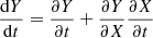 taking into account
  we find
 (A.1)
(A.1)
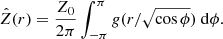
where Zis a function of cosθ and the heliocentric distance of the nucleus, r. According to assumption number 4, Z also depends on the cometocentric distance, R. Since 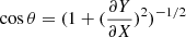 , Eq. (A.1) is a partial differential equation. How the mass loss rate Z depends on cosθ and r depends on the so-called sublimation function. The latter parameterizes how much matter sublimates from a unit area perpendicular to the incident sunlight over unit time as a function of the heliocentric distance of the comet. In this work we use a sublimation function for water ice derived by Sekanina (Sekanina 1992; Marsden et al. 1973) as follows:
![Mathematical equation: $$ \begin{aligned} g(r)=0.111262 \left(\frac{2.808}{r}\right)^{2.15} \left(1+\left[\frac{r}{2.808}\right]^{5.093} \right)^{-4.6142}, \end{aligned} $$](/articles/aa/full_html/2019/02/aa34806-18/aa34806-18-eq9.gif)
where r is heliocentric distance in astronomical units. In order to account for the fact that not every surface element of the cometary nucleus is necessarily perpendicular to the incoming sunlight the mass loss rate has to be proportional to  , where r0 is the heliocentric distance of a unit sized surface element. The mass loss rate averaged over spin period (
 ) then equals
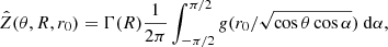
where Γ(R) describes the relative mass loss rate in the nucleus as a function of the core radius R and α is the azimuthal angle between the radius vector pointing towards the surface element and the direction of insolation. For nuclei with non-constant density, Γ(R) would be inversely proportional to the density distribution. If the changes in the shape of the comet are relatively minor over one orbit,  can finally be averaged over one orbital period to obtain the absolute mass loss rate
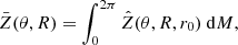
where M is the mean anomaly of the orbit of the comet.
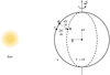 |
Fig. A.1. Anisotropic mass loss induced shape changes as described in Eq. (A.1). I and G are points on original surface of the comet, while H lies on the processed surface resulting from volatile loss, desiccation, and collapse of subsurface cavities. |
A.1. Analytical solution: Constant mass loss rates throughout the nucleus
For constant mass loss rates throughout the core Γ(R)=1, Eq. (A.1) can be solved analytically. With  the solution reads
For non-constant mass loss rates in the nucleus (Γ(R) ≠ 1) solutions to the shape evolution equations have to be found numerically. In that case all derivatives are approximated by finite differences that can be solved with a suitable algorithm.
A.2. Equation for arbitrary rotation
If the spin axis is not perpendicular to the orbital plane we represent the shape of the comet by a closed surface in spherical coordinates S(ϕ, ψ). The partial differential equation for the surface of the nucleus then reads

where θ is the angle between the surface normal at point (ϕ, ψ) and the cometocentric radial vector to point (ϕ, ψ). The results obtained by the fully numerical solution are in good agreement with the analytical solution for those cases where the spin axis is perpendicular to the orbital plane. Forward and consequent backward propagation in time returns the initial shape with negligible errors.
Appendix B: Mass loss timescale
In order to determine how long it would take cometary nuclei to evolve into the observed shapes through anisotropic mass loss, we estimate the mass loss near the equator of a comet with zero obliquity. The mass loss flux per unit area reads
where r is the heliocentric distance and Z0 represents the evaporation flux at a heliocentric distance of 1 au, where Z0 = 3 × 10¹⁷ mol cm−2 s−1 (Marsden et al. 1973). The mass loss flux averaged over one rotation period of the nucleus is
If the rotation period of the comet is much shorter than the orbital period of the comet and spin orbit resonances can be excluded, we can average the mass loss flux over one orbital period as well so that
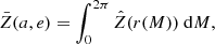
where a and e are the semi-major axis and the eccentricity of the comet’s orbit and M is the mean anomaly. The number of molecules in any given column of cometary material is

where NA is the Avogadro constant and m is the mass of the column. Since the overwhelming part of the sublimated material is water ice, w denotes the molar mass of water, and p is a coefficient that models the mean porosity of the nucleus. A rough estimate for the mass loss timescale of a comet on a heliocentric orbit with semi-major axis a and eccentricity e is
 (B.1)
(B.1)
All Figures
|
Fig. 1. Cometary nuclei imaged from spacecraft encounters or ground-based radar. Panel a: 67P/Churyumov-Gerasimenko. Image credit: ESA/Rosetta/MPS for OSIRIS Team MPS/UPD/LAM/IAA/SSO/ INTA/UPM/DASP/IDA. Panel b: 9P/Tempel 1. Image credit: PIA02142, Courtesy NASA/JPL-Caltech. Panel c: 103P/Hartley 2. Image credit: PIA13570, Courtesy NASA/JPL-Caltech. Panel d: 19P/Borelly. Image credit: PIA03500, Courtesy NASA/JPL-Caltech. Panel e: 1P/Halley. Image credit: ESA/MPS. Panel f: 81P/Wild 2, see Duxbury et al. (2004). Panel g: 8P/Tuttle. Image credit: Arecibo Observatory Planetary Radar, resolution 1 μs × 0.5 Hz, see Harmon et al. (2010). |
| In the text | |
|
Fig. 2. Shape and spin evolution of cometary nuclei can lead to bilobed shapes. |
| In the text | |
|
Fig. 3. Possible shapes of cometary nuclei as a result of anisotropic mass loss are shown for a variety of configurations. The outcome is determined by the initial obliquity of the nucleus before substantial mass loss sets in (α1) and final obliquity after destabilization of the original spin state (α2). The corresponding spin axes are red and green, respectively. The nuclei in this graph are orientated according to their final obliquity with respect to the orbital angular momentum (vertical direction). |
| In the text | |
|
Fig. A.1. Anisotropic mass loss induced shape changes as described in Eq. (A.1). I and G are points on original surface of the comet, while H lies on the processed surface resulting from volatile loss, desiccation, and collapse of subsurface cavities. |
| In the text | |
Current usage metrics show cumulative count of Article Views (full-text article views including HTML views, PDF and ePub downloads, according to the available data) and Abstracts Views on Vision4Press platform.
Data correspond to usage on the plateform after 2015. The current usage metrics is available 48-96 hours after online publication and is updated daily on week days.
Initial download of the metrics may take a while.