| Issue |
A&A
Volume 622, February 2019
|
|
|---|---|---|
| Article Number | A108 | |
| Number of page(s) | 12 | |
| Section | Numerical methods and codes | |
| DOI | https://doi.org/10.1051/0004-6361/201834555 | |
| Published online | 05 February 2019 | |
Extending the event-weighted pulsation search to very faint gamma-ray sources
Laboratoire Leprince-Ringuet, Ecole polytechnique, CNRS/IN2P3, 91128 Palaiseau, France
e-mail: This email address is being protected from spambots. You need JavaScript enabled to view it.
Received:
1
November
2018
Accepted:
17
December
2018
Abstract
Context. Because of the relatively broad angular resolution of current gamma-ray instruments in the MeV–GeV energy range, the photons of a given source are mixed with those coming from nearby sources or diffuse background. This source confusion seriously hampers the search for pulsation from faint sources.
Aims. Statistical tests for pulsation can be made significantly more sensitive when the probability that a photon comes from the pulsar is used as a weight. However, computing this probability requires knowledge of the spectral model of all sources in the region of interest, including the pulsar itself. This is not possible for very faint pulsars that are not detected as gamma-ray sources or whose spectrum is not measured precisely enough. Extending the event-weighted pulsation search to such very faint gamma-ray sources would allow improving our knowledge of the gamma-ray pulsar population.
Methods. We present two methods that overcome this limitation by scanning the spectral parameter space, while minimizing the number of trials. The first one approximates the source to background ratio yielding a simple estimate of the weight while the second one makes use of the full spatial and spectral information of the region of interest around the pulsar.
Results. We tested these new methods on a sample of 144 gamma-ray pulsars already detected by the Fermi Large Area Telescope data. Both methods detect pulsation from all pulsars of the sample, including the ones for which no significant phase-averaged gamma-ray emission is detected.
Key words: gamma rays: general / pulsars: general / methods: data analysis / methods: statistical
© ESO 2019
 Open Access article, published by EDP Sciences, under the terms of the Creative Commons Attribution License (http://creativecommons.org/licenses/by/4.0), which permits unrestricted use, distribution, and reproduction in any medium, provided the original work is properly cited.
1. Introduction
One of the important contributions of the Fermi Large Area Telescope (LAT; Atwood et al. 2009) to gamma-ray astronomy is the detection of many pulsars. Prior to the Fermi launch in 2008, at most ten gamma-ray pulsars were known (Thompson 2008). Ten years later, more than 200 have been detected1, representing the most abundant Galactic source class at GeV energies (Acero et al. 2015). Detecting more pulsars, especially faint ones, is very important to characterizing as well as possible the gamma-ray pulsar population.
One way of finding gamma-ray pulsars is to search for periodic emission after phase-folding gamma-ray data with rotation ephemerides, obtained from contemporaneous timing observations conducted in radio or X-rays. Prior to Fermi’s launch, a pulsar timing consortium (PTC) was organized to support LAT observations of pulsars by providing accurate pulsar ephemerides (Smith et al. 2008). Another way of finding gamma-ray pulsars is to look at LAT catalog unassociated sources with a pulsar-like spectrum (see e.g. Clark et al. 2017; Pleunis et al. 2017) but, by construction, it does not target very faint gamma-ray sources. We thus focus on the former approach in the rest of this paper.
The sensitivity to pulsation depends on the purity of the event sample, which depends on the level of background and on the instrument performance, especially its angular resolution. In the MeV–GeV energy range, the Galactic diffuse emission is bright and is the main source of background for candidate pulsars near the Galactic plane. Neighbouring sources can also significantly increase the level of background because of the finite angular resolution of the instrument. The LAT point spread function (PSF) at low energy is driven by multiple scattering of the electron and positron created by pair-conversion of the photon in the tracker. The 68% containment angle ranges from 5.5° at 100 MeV to 0.1° at 30 GeV (Atwood et al. 2009).
As shown in Bickel et al. (2008) and Kerr (2011), it is possible to efficiently mitigate the background problem by weighting the pulsation statistical test with the probability of each event to come from the pulsar position. To compute the exact probability, one needs a complete description of the region of interest (RoI) around the pulsar (large enough to fully take into account the effects of the PSF), including the spectral model of all gamma-ray sources in the RoI. So one prerequisite is to be able to measure the spectrum of the candidate pulsar, which is usually done by performing a maximum-likelihood fit of the RoI. When the fit leads to a clear detection of the pulsar, its spectrum is well measured and the photon probabilities can be computed. On the contrary, a weak detection of the pulsar or obviously its non detection precludes a good measurement of its spectrum. As a consequence, current event-weighted methods to search for pulsation cannot be applied to very faint gamma-ray sources.
The only possible way to overcome this limitation is to scan over the pulsar spectral parameters in order to find the ones maximizing the statistical test used to search for periodic emission. The obvious drawback is that the resulting significance must be corrected for the number of trials performed during the scan. Consequently, the challenge of extending the event-weighted methods to very faint pulsars consists of minimizing the number of trials when scanning the spectral parameter space, while maximizing the pulsation sensitivity, that is, getting as close as possible to the spectral parameters yielding the optimal weights.
After presenting in Sect. 2 the statistical test we used for pulsation searches, we present in Sect. 3 a method using a simple weight definition that does not involve a detailed spatial nor spectral modelling of the RoI. In Sect. 4, we describe a more complex method that takes advantage of the complete knowledge of the RoI and the full capabilities of the instrument.
Both methods are tested on a sample of 144 known LAT pulsars. This sample comprises the 117 pulsars from the LAT Second Gamma-ray Pulsar Catalog (2PC; Abdo et al. 2013), among which only two are not significant gamma-ray sources when analysing eight years of LAT data. Adding 27 post-2PC detected pulsars (Hou & Smith 2014; Laffon et al. 2014; Smith et al. 2017) to our sample increases the number of faint pulsars to 12. The results, based on the analysis of 8 year of Pass 8 SOURCE class data (Atwood et al. 2013; Bruel et al. 2018), are presented and discussed in Sect. 5.
2. The event-weighted H-test
To test the signal periodicity, we use the weighted H-test derived by Kerr (2011) from the original H-test proposed by de Jager et al. (1989):
![Mathematical equation: $$ \begin{aligned} H_{m{ w}} = \mathrm{max} \left[ Z_{i{ w}}^2 -c \times (i-1)\right], \quad 1\le i \le m \end{aligned} $$](/articles/aa/full_html/2019/02/aa34555-18/aa34555-18-eq1.gif) (1)
(1)
The weighted H-test definition involves the weighted  test:
test:
 (2)
(2)
where
 (3)
(3)
and
 (4)
(4)
where the sums run over the list of N photons with pulsar rotational phase ϕi and weight wi.
In the following, we have adopted the H-test parameter recommended values m = 20 and c = 4 (since they provide an omnibus test) and write Hw instead of H20w. We note that one property of  and Hw is that they are not sensitive to a global scaling of the photon weights.
The analytic, asymptotic null distribution of Hw has been derived by Kerr (2011). Because we want to use Hw even with small event samples, we derive this distribution directly with Monte Carlo simulations, allowing us to know, for any x > 0, the probability P(Hw > x), that Hw evaluated on a non-periodic sample can fluctuate to values larger than x. The calibration procedure is described in Appendices A and B. We show that P(Hw > x) can be parameterized as a function of the sum of the weights, computed under the prescription that the maximum weight is one.
Rather than using directly  , the measured value of Hw, when searching for pulsation, we use instead
  , that we name pulsation significance for simplicity’s sake. We note that the relation between Pw and nσ, the significance expressed in number of σ, is given by
  . The 3, 4, and 5σ levels correspond to Pw ∼ 2.57, 4.20 and 6.24, respectively.
3. Simple weights
Let us consider an RoI centered on a pulsar. The probability that a photon originates from the pulsar depends on the position and spectrum of all gamma-ray sources in the ROI and the response functions of the instrument. We assume that all sources are steady and that the pulsar spectrum does not depend on phase. For a photon at a position Ω with an energy E, the probability that it comes from the pulsar is the ratio of the pulsar differential rate, rpsr, and the total differential rate at this energy and position. Defining rbkg as the sum of all but the pulsar differential rates, we have:
 (5)
(5)
3.1. Simple weight definition
Since we are interested in very faint pulsars, we assume that the pulsar differential rate is negligible compared to rbkg. Let us also assume that the background only comprises an isotropic diffuse emission. The background differential rate thus depends only on the energy E and we have:
 (6)
(6)
We note that the resulting weight w is directly proportional to the pulsar absolute flux. Since the event-weighted statistical tests are unchanged when all weights are scaled by a constant, in the limit of very faint pulsars only the shape of the pulsar spectrum matters and not its absolute flux normalization. We also note that the weight position dependence only comes from the pulsar differential rate. Since the pulsar is a point source, the position dependence is described by the instrument PSF.
We can rewrite the weight as the product of two functions:
 (7)
(7)
where g(E,Ω) contains all the position dependence and is defined such that it is 1 at the pulsar position at all energies. f(E) is the weight at the pulsar position and depends on the pulsar and background spectral shapes and on the energy dependent part of the PSF normalization. The maximum of f(E) is set to one to follow the maximum weight prescription mentioned in Sect. 2.
At a given energy, the LAT PSF is well approximated by a Moffat profile (Moffat 1969)2:
 (8)
(8)
where x is the angular distance to the source and s a scale parameter.
The integral  and we note that the integral up to a distance of 3s is about 0.68, so that the parameter s corresponds to a third of the PSF 68% containment angle. We can thus write the function g(E,Ω) as
 (9)
(9)
where σpsf(E) is the energy dependent PSF 68% containment angle, which for the LAT Pass 8 SOURCE event class can be parameterized as follows (Ackermann et al. 2013):
 (10)
(10)
with p0 = 5.11°, p1 = −0.76, p2 = 0.082° and E in MeV and the addition is in quadrature.
The weight position-independent part, f(E), corresponds to the weight at the position of the pulsar. Its computation is made simple by the fact that both the pulsar and background rates involve the same instrument effective area, which cancels out in Eq. (6). As a consequence f(E) can be computed directly using the pulsar and background spectral shapes, as well as the energy dependent part of the PSF normalization (1/4πs2 in Eq. (8)).
As shown in Abdo et al. (2013), the spectral shape of pulsars between 60 MeV and 60 GeV energy range can be modelled with a power law with an exponential cutoff:
 (11)
(11)
with, for most of pulsars, an index γ ranging from 0.5 to 2, an energy cutoff Ec between 0.6 and 6 GeV (and β set to 1 in 2PC). We consider three (γ, Ec) test-cases: (2.0, 0.6 GeV), (0.5, 0.6 GeV) and (2.0, 6 GeV). The latter two encompass the bulk of the pulsars, while the first one corresponds to pulsars whose pulsation is driven by low energy photons.
Regarding the background spectral shape, we use the spectrum of the Galactic diffuse emission towards the Galactic center. It can be modelled with a smoothly broken power law, with spectral indices of ∼1.6 and ∼2.5 below and above ∼3 GeV, respectively3.
Figure 1 shows f(E) for the three pulsar test-cases. Expressed as a function of log10E, the function f is Gaussian-like. The pulsar energy cutoff is responsible for the decrease of f at high energy. At low energy, its decrease is mainly driven by the increase of the instrument PSF. The center position parameter μw is located between 2.5 and 4.5 (corresponding to 30 MeV and 30 GeV, respectively) while the half 68% width parameter σw ranges from 0.3 to 0.45.
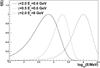 |
Fig. 1. Weight position independent part f(E) for three test pulsar spectra. |
This result does not change qualitatively when using the spectrum of the Galactic diffuse emission at high Galactic latitude: for a given pulsar spectrum, changing the background spectral index moves the peak position of f(E) but its shape remains Gaussian-like, with a width in the same [0.3,4.5] range. As a consequence, we can use the same weight definition for young pulsars, that are mostly near the Galactic ridge, and millisecond pulsars, that tend to lie at high Galactic latitude.
We approximate f(E) with a Gaussian in log10E:
 (12)
(12)
We note that the examples in Fig. 1 are not exactly Gaussian. Using other functional forms that better model the negative tail of f(E) does not improve the performance of the pulsation search, that is, better matching of f(E) does not compensate for the simple assumptions that we use (very faint source on top of an isotropic background). Similarly, in Sect. 4.1 we show that refining the PSF information fails to improve the performance.
The Gaussian definition of f(E) introduces two parameters, μw and σw. Formally, one would have to scan over these two parameters in order to fully explore the pulsar spectral parameter space. However, σw varies much less than μw, allowing us to fix σw and to vary only μw. We note that the σw range was obtained under the very faint pulsar hypothesis. For brighter pulsars, the energy range over which the pulsar emission is significant is larger, leading to a wider shape for f(E), which corresponds to larger values of σw. For this reason, we chose to fix σw to 0.5. We describe our checks that, on average, this choice is valid for all pulsars in Sect. 5.
Thus, the simple weight definition that we propose is:
 (13)
(13)
3.2. Simple weight scan
For a given value of μw, we can compute Hw and the corresponding pulsation significance Pw using the weights w(E, x, μw). Figure 2 shows Pw as a function of μw for PSR J1646−4346 (Smith et al. 2017). We chose this pulsar to illustrate the method because it is one of the pulsars in our sample that are not detected as a gamma-ray source with eight years of LAT data and, as a consequence, for which the original Kerr (2011) method can not be applied.
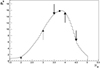 |
Fig. 2. Pulsation significance as a function of μw for PSR J1646−4346. The upward arrows correspond to the first three trials, while the downward arrows correspond to the two subsequent trials. The sixth trial, shown with a circle, is the maximum of the Gaussian passing through the three points corresponding to the thick-line arrows. |
As can be seen in this example, Pw(μw) has a Gaussian shape around its maximum. This shape is simply the result of the relative matching between the weights w(E, x, μw) and the optimal weights, when μw varies. We refer to the maximum position and the 68% width of Pw(μw) as μP and σP, respecively. Figure 3 shows the distribution of σP versus μP for the 144 pulsar sample. The bulk of the pulsars have 3 < μP < 4 while a few have a low μP, corresponding to a pulsation signal driven by low energy photons (e.g. PSR J1513−5908, aka PSR B1509−58 (Abdo et al. 2010; Kuiper et al. 2017), whose energy cutoff is below 30 MeV). The width σP is between 0.35 and 0.9.
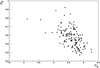 |
Fig. 3. 68% width as a function of the peak position of Pw(μw) for the 144 pulsar sample. |
Searching for pulsation consists in finding the maximum of Pw(μw). The easiest way to do so is to perform a very fine scan over μw but that would lead to a too large number of trials. Taking advantage of the Gaussian-shape of Pw(μw) around its maximum, we performed the following algorithm (illustrated in Fig. 2):
-
Test three values of μw = (2, 3, 4). Let μ0 be the one giving the maximum Pw.
-
Test two more values of μw = (μ0 − 0.5, μ0 + 0.5). The 0.5 distance is chosen such that it is of the order of the minimum of the 68% width of Pw(μw). Let μ1 be the one giving the maximum of Pw among all the trials with 2 ≤ μ ≤ 4;
-
Test μw = μg, the position of the maximum of the Gaussian passing through the three points μ1 − 0.5, μ1, μ1 + 0.5 (all tested in the previous steps);
The resulting pulsation significance of the simple method, corrected for the 6 trials, is:
 (14)
(14)
We note that the six trials are partially correlated, especially the ones with a small difference in μw. Unfortunately there is no simple way to estimate and take into account these correlations when correcting the pulsation significance and so we simply ignored them and adopted the conservative definition of Ps given by Eq. (14).
4. Model weights
To increase the sensitivity of the pulsation search, one has to go beyond the simple weight definition of Eq. (13). There are two possible approaches: (1) use the spatial and spectral description of all sources in the RoI; (2) take into account the full PSF information. While the former requires precise RoI modelling including spectral fits, the latter can be achieved by a minimal change of the weight definition, as it is a consequence of a refinement of the PSF definition.
4.1. PSF event types
One of the new features of Pass 8 (Atwood et al. 2013), the latest version of the reconstruction and selection of LAT data, is the introduction of the PSF event types. Prior to Pass 8, the events of a given class (e.g. SOURCE class) were divided into two subclasses, FRONT and BACK, depending on the location of the photon pair-conversion in the LAT tracker. Because of the different thicknesses of the converters in these two sections of the tracker, the PSF of the two subclasses are significantly different: at 1 GeV the FRONT and BACK PSF 68% containment angles are 1.2 and 0.61°, respectively. In Pass 8, thanks to a multivariate analysis, the events are divided into four event types PSF0, PSF1, PSF2 and PSF3, ordered in decreasing quality of the reconstructed direction, with a PSF 68% containment angle at 1 GeV of 1.8, 1.0, 0.66 and 0.42°, respectively.
It is straightforward to take into account the PSF events types in the context of the simple weight definition of Eq. (13): one just has to properly modify the f(E) part of the weight induced by the 1/4πs2 factor of the normalization of the Moffat profile (Eq. (8)). We note that this modification is made simple by both the faint-source and uniform-background hypotheses.
Tested on LAT data, this modification failed to clearly increase the pulsation significance of known pulsars. This failure can be explained by two reasons. First, as soon as the faint-source hypothesis does not hold, the correction induced by the 1/4πs2 factor of the Moffat profile normalization is not correct: in the extreme situation in which the background is negligible, all photons should have a weight of approximately one, regardless of their PSF event type.
Moreover, taking into account the better PSF description given by the PSF event types is in fact equivalent to a better spatial description of the RoI. This improvement might not be large enough to compensate the crude approximation of the uniform-background hypothesis. In other words, one has to use a precise spatial and spectral description of the RoI to take full advantage of the additional information provided by the PSF event types. As a consequence, going beyond the simple weights presented in the previous section requires the full spatial and spectral description of the RoI around the pulsar.
4.2. Pulsar RoI description
To compute the weights for each pulsar, we performed a binned maximum-likelihood fit, following the standard Fermi/LAT analysis procedure, of the 10.05 × 10.05° RoI centered on the pulsar, with a pixel size of 0.05°. We used 37 bins in log10E, between 63.1 MeV and 316.2 GeV.
We included in the source model the following components:
-
the Galactic diffuse emission and the isotropic template (that accounts for the isotropic diffuse emission as well as the residual background)4;
-
all point-like and extended sources from the preliminary eight-year Fermi/LAT source list (FL8Y)5, within five degrees of the RoI border.
If the closest point source to the pulsar is within a distance of 1.5 times the source 95% error radius, we considered the source to be the pulsar and set its position to the pulsar position. Otherwise we added a new source at the pulsar position.
We performed the maximum-likelihood fit with SOURCE class events (combining all PSF event types) above 160 MeV whose zenith angle is less than 90° to avoid Earth limb contamination, collected between 2008 August 4 and 2016 August 2. The significance of each source in the model is estimated using the test statistic, TS, defined as twice the difference in log-likelihood obtained with and without the source. A TS = 25 corresponds to ∼4σ significance (Mattox et al. 1996). The 160 MeV energy threshold for the maximum-likelihood fit has been chosen to mitigate the effect of systematic errors due to our imperfect knowledge of the Galactic diffuse emission.
Using the model derived by the fit, we built for each PSF event type the 3D map (sky position and energy) of the number of predicted events coming from the pulsar as well as the 3D map of the total number of predicted events. We were then able to compute the weights by simply dividing the former map by the latter map.
When computing Hw, we assigned to each event the weight of the bin corresponding to the event position and energy of the 3D map corresponding to the PSF event type of the event. In Kerr (2011), the weights are computed using the Fermi/LAT Science Tool gtsrcprob6 that assigns to each event the probability that the event belongs to a given source of the RoI. Our binned approach is less CPU intensive and the chosen binning is fine enough to not induce any significant loss of sensitivity.
4.3. Spectral parameter scan
For bright gamma-ray pulsars, the maximum-likelihood fit gives a large TS for the pulsar and its spectral parameters are well estimated. We were thus able to use these spectral parameters to compute the weights, as done in Kerr (2011). On the contrary, for faint pulsars (TS < 25) or pulsars just above the TS = 25 threshold for which the spectrum is not precisely estimated, we have to scan over the spectral parameters.
Instead of using Eq. (11) to model the power law with an exponential cutoff, we used the following expression:
 (15)
(15)
as used in FL8Y and the forthcoming 4FGL catalog, with β given by the fit for bright pulsars or fixed to 0.667 for faint or not-detected ones. The formal change between the energy cut off and parameter a is convenient to scan the spectral parameter space, as will be shown later.
For a given set of (a, γ), we fix the corresponding spectral parameters and perform the maximum-likelihood fit with the pulsar normalization being the only free parameter. If TS < 4, we set the normalization to the 68% confidence limit. Using the resulting pulsar spectrum, we compute the four PSF event type weight maps and compute the pulsation significance, taking into account the PSF event type information by using for each event the PSF event type weight map corresponding to the event. Figure 4 shows how the pulsation significance varies in the (a, γ) plane for PSR J1646−4346.
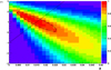 |
Fig. 4. Pulsation significance in the (a, γ) parameter space normalized relative to its maximum for PSR J1646−4346. The dashed contour line corresponds to the 90% level. The solid straight line corresponds to the line Lm along which a scan is performed to obtain the model weight pulsation significance, as described in Sect. 4.4. |
The iso-level contours are elliptical. Let us consider the high Pw region corresponding to Pw larger than 90% of the maximum, whose ellipse-like contour is named ℰ90. To characterize ℰ90, we use the lowest and highest a extremities of ℰ90. These points are shown in Fig. 5 for the 144 pulsar sample. The important result is that the lowest and highest a points of ℰ90 are not mixed and it is possible to define a line separating them.
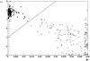 |
Fig. 5. Position of the lowest (dots) and highest (crosses) a points of ℰ90 (the region of the (a, γ) plane with Pw larger than 90% of the maximum) for the 144 pulsar sample. The solid line corresponds to the line Lm along which a scan is performed to obtain the model weight pulsation significance, as described in Sect. 4.4. |
The fact that ℰ90 is clearly elongated along a direction that tends to go from the upper-left to the lower-right of the (a, γ) plane is the consequence of how the weights vary with the spectral parameters. For a given background spectrum, when a increases, the effective position of the spectrum cutoff decreases and the energy position of the maximum weight at the pulsar position shifts to lower energy. On the other hand, the maximum weight energy position shifts to higher energy when γ decreases. So when a increases and γ decreases, the two effects partly counterbalance each other and the maximum weight energy position does not vary very much. The situation is reversed along the minor axis of ℰ90: the increases of a and γ both shift the maximum weight energy position to lower energy. This is why ℰ90 is very eccentric. We note that the convenient elliptical shape of the high Pw region is the result of the change from Eq. (11) to (15) to model the power law with an exponential cutoff.
4.4. Model weight scan
As for the simple weight method, the goal is to find the maximum of Pw in the lowest possible number of trials. The characterization of the high Pw region obtained in the previous section naturally suggests a two-step procedure: first finding the major-axis of ℰ90 then scanning along the major-axis to find the maximum Pw.
To find the major-axis of ℰ90 we performed a scan along the line Lm, going from (a = 0, γ = −1) to (a = 0.03, γ = 3), that crosses almost all ℰ90, as shown in Fig. 5. The choice of Lm is motivated by the fact that increasing both a and γ at the same time allows a fast variation of the maximum weight energy position and, therefore, an efficient exploration of the pulsar spectrum parameter space. This choice might be slightly refined in the future thanks to the analysis of a larger sample of gamma-ray pulsars.
An example of the Lm scan is shown in Fig. 6. Because the Pw variation along Lm is Gaussian-like around the maximum, we can perform a similar six-trial algorithm as for the simple weight method, with the following test positions:
-
Test three values of a = (0.005, 0.015, 0.025). Let a0 be the one giving the maximum Pw.
-
Test two more values of a = (a0 − 0.005, a0 + 0.005). The 0.005 distance is chosen such that it is of the order of the minimum of the 68% width of Pw(a) when scanning along Lm. Let a1 be the one giving the maximum of Pw among all the trials with 0.005 ≤ a ≤ 0.025;
-
Test a = ag the position of the maximum of the Gaussian passing through the three points a1 − 0.005, a1, a1 + 0.005 (all tested in the previous steps);
-
Let Am(am, γm) be the point giving the maximum Pw among the six trials.
We expect Am to lie on the major-axis and we need one more point to define it. Figure 7 shows γ0, the intercept of the major-axis with the γ-axis, as a function of am. The correlation between the two can be modelled with γ0 = 0.4 + 100am. We used this correlation to choose the point A0(a, γ)=(0, 0.4 + 100am) that, together with Am, defines the major axis LM.
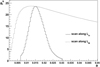 |
Fig. 6. Pulsation significance as a function of a, when scanning along Lm (solid line) and along LM (dashed line) for PSR J1646−4346. Lm and LM are two straight line in the pulsar parameter space (a, γ). Lm goes from (a = 0, γ = −1) to (a = 0.03, γ = 3) while LM approximates the ℰ90 major-axis. |
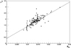 |
Fig. 7. Correlation between γ0, the intercept of the ℰ90 major axis with the a = 0 axis, and am, the position of the maximum Pw along Lm for the 144 pulsar sample. The solid line shows the γ0 = 0.4 + 100am parameterization. |
An example of the Pw variation along LM is shown in Fig. 6. The LM scan allows us to reach a higher Pw than the Lm scan, but, because the latter goes through ℰ90, the gain in Pw is rather modest (less than 10% by definition of ℰ90). To optimize the definition of the second step, we look at the maximum relative gain in Pw along LM versus its relative position with respect to am. As can be seen in Fig. 8, the gain in Pw is on average about 1%, reaching at most 5% for few pulsars. Regarding the optimal position a, it can be either smaller or larger than am. This would imply at least two more trials, on top of the six ones already performed during the Lm scan, inducing an additional trial correction of log10(8/6)=0.125.
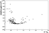 |
Fig. 8. Maximum Pw gain along LM as a function of its relative position with respect to am for the 144 pulsar sample. |
For pulsars on the verge of pulsation detection, that is, at the 4σ level, corresponding to Pw ∼ 4.2, the additional trial correction corresponds to about 2% of Pw, larger than the average 1% gain of the LM scan. As a consequence, we chose not to perform the LM scan. The model weight pulsation significance corrected for the six trials is thus:
 (16)
(16)
As in the simple weight method, the six trials are partially correlated and, for the same reasons, we choose to ignore them and to use a conservative definition of Pm.
5. Results
To test the performance of the simple and model weight methods, we applied them to the sample of 144 LAT pulsars (117 pulsars from 2PC and 27 post-2PC detected pulsars). For each pulsar, we performed the binned maximum-likelihood fit presented in Sect. 4.2 to estimate the TS of the pulsar and computed the model weights. 12 pulsars are found to have TS < 25.
To perform the pulsation search, we selected Pass 8 SOURCE class events within five degrees of the pulsar above 60 MeV. We used the Fermi plugin (Ray et al. 2011) to the pulsar timing software TEMPO2 (Hobbs et al. 2006; Edwards et al. 2006) and the pulsar ephemeris provided by the PTC (Smith et al. 2008, 2019) to convert the event arrival time into a pulsar rotational phase. The pulsation probabilities are computed using only the data collected during the validity period of the ephemerides.
We also compared the simple and model weight results to that obtained with the original Kerr (2011) method, which simply corresponds to the model weight method with the weights computed using the spectral parameters given by the maximum-likelihood fit. This is possible only when the source is significantly detected by the fit, meaning when TS > 25. We named the corresponding pulsation significance Pfit. Compared to Pm, Pfit has the obvious advantage of being the result of only one trial.
To compare the performance of the new methods to a standard unweighted pulsation search, we also performed a grid search, with each grid point corresponding to a set of cuts in energy and distance to the pulsar. We used the grid parameters defined by Kerr (2011), where it is reported that the event weighting method improves the pulsation sensitivity by a factor 1.5–2.
5.1. Model weights
The pulsation significance Pm obtained with the model weights is shown in Fig. 9 as a function of TS. All 144 pulsars have Pm > 5.4, corresponding to 4.6σ. The general trend is that Pm on average increases with TS. This is not surprising since, on average, the larger the TS, the stronger the pulsation signal. The scatter around this trend is mainly due to the pulse shape diversity. The most interesting result is the clear detection of pulsation from all pulsars with TS ≲ 50, which proves that the model weight method is able to detect pulsation even when the pulsar spectrum information is not available or not fully reliable. The Pm and Ps values are given in Table 1 for the 12 pulsars with TS < 25. Ignoring the PSF event type information when computing the model weights leads to a loss of sensitivity that decreases with TS, from 20% on average for faint pulsars to 10% for the brightest.
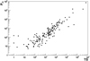 |
Fig. 9. Model weight pulsation significance Pm as a function of TS for the 144 pulsar sample. Pulsation is detected for all pulsars, including the pulsars with TS < 25, whose results are reported in Table 1. |
Results of the TS < 25 pulsars: TS of the spectral fit, model and simple weight pulsation significances, Pm and Ps.
The comparison between Pm and Pfit is shown in Fig. 10. On average the model weight method provides the same pulsation significance, within ∼5% for most of the pulsars. Only one has Pm lower than Pfit by more than 10%.
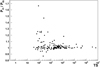 |
Fig. 10. Comparison of the model weight pulsation significance, Pm, and the pulsation significance derived when using the pulsar spectrum given by the spectral fit, Pfit, as a function of TS for the 131 pulsars with TS > 25 out of the 144 pulsar sample. The two methods give on average the same result but the model weight method is more sensitive by at least 20% for eight pulsars, whose results are reported in Table 2. |
Pulsars with TS > 25 and Pm/Pfit > 1.2.
On the contrary, the model weight method often improves significantly over Pfit, with a gain greater than 20% for eight pulsars. These eight pulsars all have TS > 60 so it is unlikely that the improvement is explained by a poor estimation of the spectral parameters by the fit. A possible explanation is the presence of a significant off-pulse emission: the spectral parameters derived by the fit correspond to the spectrum of the sum of the pulsed and unpulsed gamma-ray components and not to the pulsed component alone, while the model weight method is able to find spectral parameters closer to the pulsed component spectrum.
As reported in Abdo et al. (2013), 34 2PC pulsars have a significant off-peak emission, whose spectrum is compatible with a simple power-law spectrum for 13 of them. Moreover, the off-peak emission of these 13 pulsars is generally soft, with a spectral index of approximately two. A flat and soft off-peak emission that is not negligible compared to the pulsed emission could lead to a total emission spectrum significantly different from the pulsed emission spectrum. Investigating that it is also the case of the largest Pm/Pfit pulsars would require performing the analysis of the off-pulse emission, which is out of the scope of this paper and will be presented in the forthcoming third LAT Gamma-ray Pulsar Catalog (3PC).
We instead estimated the significance of the curvature of the spectrum. As in Abdo et al. (2013) and Acero et al. (2015) we performed a maximum-likelihood fit assigning the pulsar a power-law spectrum and compute σcurv = (TS − TSPL)−1/2, where TS and TSPL correspond to the maximum-likelihood fit of a power-law with and without exponential cutoff, respectively. We note however that σcurv measures the significance of the curvature and not how flat or soft the spectrum is.
A very simple and crude estimator of the softness and flatness of the spectrum is provided by the sum S = γ + log10Ec, with Ec = a−1/β. This estimator can be improved by taking into account the correlation between γ and log10Ec. The analysis of the distribution of γ vs log10Ec for the 144 pulsar sample yields a positive correlation with a slope ∼1.418 and the projection along the first principal axis is Sf = 0.576γ + 0.817log10Ec. In the case of a spectrum without significant curvature, the spectral parameters γ and Ec are not precisely measured. To take into account this case, we replace γ and Ec by their 68% upper limit and define the following simple “soft–and–flat” estimator:
 (17)
(17)
Figure 11 shows the ratio Pm/Pfit as a function of Sf. Although the correlation between these two quantities is not perfect, we note that all the eight pulsars with Pm/Pfit > 1.2 lie in the right-hand tail of the Sf distributions, meaning that their spectra are among the most soft and flat of the sample. Some of their properties are given in Table 2. Only two of them have a curvature significance above 4σ: J0742−2822 and J1828−1101 with σcurv = 8 and 4.9, respectively. All the others have γ > 2.4. We note that only four of these eight pulsars are in 2PC and only two are detected as a gamma-ray source (J0742−2822 and J1410−6132). Out of these two, only J1410−6132 is reported to have a significant off-peak emission.
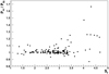 |
Fig. 11. Comparison of the model weight pulsation significance, Pm, and the pulsation significance derived when using the pulsar spectrum given by the spectral fit, Pfit, as a function of the “soft–and–flat” estimator Sf for the 131 pulsars with TS > 25 out of the 144 pulsar sample. The eight pulsars with Pm/Pfit > 1.2 are among the pulsars with the largest Sf, meaning those with the softest and flattest spectrum. |
The comparison of the model weights with the grid search is shown in Fig. 12 as a function of TS for the 144 pulsar sample. We confirm the improvement of the weighting method over the unweighted approach, with a gain in sensitivity larger than two for the TS < 25 pulsars.
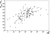 |
Fig. 12. Comparison of the pulsation significance obtained with an unweighted approach, Pgrid, and the model weight pulsation significance, Pm, as a function of TS for the 144 pulsar sample. The improvement of the model weight method over the unweighted approach is large, especially for the lowest TS pulsars. |
5.2. Simple weights
The comparison between the simple weights and the model weights is shown in Fig. 13. As expected, the simple weights are less powerful than the model weights. The difference in performance decreases from about 30% for the brightest pulsars to an average of about 15% at TS ∼ 300. This difference never goes beyond 40%. This difference is relatively small given the simplicity of the simple weight implementation compared to the complex procedure of the model weights. The Ps values are given in Table 1 for the 12 pulsars with TS < 25. Except for a few of the brightest pulsars, the simple model performs better than the standard grid search, especially for TS ≤ 100 where Ps is greater than Pgrid by at least 40%.
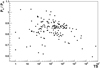 |
Fig. 13. Comparison of the simple and model weight pulsation significances as a function of TS for the 144 pulsar sample. The simple weight method is on average ∼15% less sensitive than the model weight method. |
When defining the simple weights in Sect. 3.1, we set σw = 0.5. To validate this choice, we perform a scan over σw between 0.2 and 0.95, with a 0.05 step. For each pulsar and each value of σw, we compute r(σw), the ratio of Ps divided by the maximum Ps reached over the σw scan. The average over the 144 pulsar sample of this ratio as a function of σw is shown in Fig. 14, as well as the lowest ratio, that is, corresponding to the pulsar for which the choice of σw is the worst. The two quantities have a maximum between 0.5 and 0.6 and do not vary much around the maximum, which validates the σw = 0.5 choice.
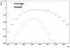 |
Fig. 14. Average (solid) and lowest (dashed) ratio r(σw) over the 144 pulsar sample as a function of σw. For each σw, r(σw) is the ratio of Ps divided by the maximum Ps reached over the σw scan. |
To summarize the results, we show in Fig. 15 the comparison of all methods that allows a clear ranking of the pulsation search methods, from the least sensitive un-weighted grid scan to the most powerful Kerr (2011) and model weight methods, with the latter, contrary to the former, being able to detect pulsation from very faint pulsars.
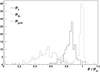 |
Fig. 15. Ratio of the pulsation significance with respect to Pm for the simple weights (solid), original event weight (dotted) and the grid search (dashed), for the 144 pulsar sample. |
We note that both the simple and model weight approaches can be used at other wavelengths (e.g. X-ray and TeV bands) but they need to be adapted to the specific context of each wavelength, taking into account the pulsar spectral parameter phase space, the PSF energy dependence and the typical background spectrum. In the case of the simple weight method, the derived general shape of f(E) may be very different from the Gaussian-like one obtained for the LAT energy band.
6. Conclusion
We show that it is possible to extend the event weighting technique to very faint gamma-ray sources when searching for pulsation and presented two approaches. The first one, the simple weight method, uses a very simple definition of the weights while the second one, the model weight method, fully takes into account the spatial and spectral information of the RoI around the pulsar. The key point for both methods is to explore efficiently the pulsar spectral parameter space, which is done with only six trials.
The model weight method reaches the same perfomance as the original event weighting method that was not applicable to the very faint gamma-ray sources. It can even be more powerful in the case of pulsars with a significant off-pulse emission.
The simple weight method is less sensitive than the model weight one but the loss of sensitivity is only ∼30% for faint sources. So this simple approach can be very useful, especially since it is straightforward to implement and is much less CPU intensive.
As a consequence the model weights method is on average the most sensitive method. It works for all pulsars (faint or bright, with or without off-pulse emission) and naturally benefits from any improvement of the instrument performance (e.g. Pass 8 PSF event types).
After ten years in orbit, Fermi/LAT continues to take data that are folded with the updated ephemerides provided by the Pulsar Timing Consortium. The two new methods presented in this paper are designed to help to detect new gamma-ray pulsars, including very faint ones, allowing us, for instance, to further test the existence of a spin-down power “deathline” (Smith et al. 2019) below which pulsars might cease to produce gamma-ray emission.
Formerly referred to as King profile in https://fermi.gsfc.nasa.gov/ssc/data/analysis/documentation/Cicerone/Cicerone_LAT_IRFs/IRF_PSF.html
The spectral indices are estimated using the Fermi/LAT Galactic diffuse emission model gll_iem_v06.fits available at https://fermi.gsfc.nasa.gov/ssc/data/access/lat/BackgroundModels.html.
Acknowledgments
We thank our Fermi/LAT collaborators Toby Burnett, Lucas Guillemot, David Smith and Matthew Kerr for fruitful discussions. The Nançay Radio Observatory is operated by the Paris Observatory, associated with the French Centre National de la Recherche Scientifique (CNRS). The Parkes radio telescope is part of the Australia Telescope 533 which is funded by the Commonwealth Government for operation as a National Facility managed by CSIRO. We thank our colleagues for their assistance with the radio timing observations. The Lovell Telescope is owned and operated by the University of Manchester as part of the Jodrell Bank Centre for Astrophysics with support from the Science and Technology Facilities Council of the United Kingdom. The Fermi/LAT Collaboration acknowledges generous ongoing support from a number of agencies and institutes that have supported both the development and the operation of the LAT as well as scientific data analysis. These include the National Aeronautics and Space Administration and the Department of Energy in the United States, the Commissariat à l’Energie Atomique and the Centre National de la Recherche Scientifique / Institut National de Physique Nucléaire et de Physique des Particules in France, the Agenzia Spaziale Italiana and the Istituto Nazionale di Fisica Nucleare in Italy, the Ministry of Education, Culture, Sports, Science and Technology (MEXT), High Energy Accelerator Research Organization (KEK) and Japan Aerospace Exploration Agency (JAXA) in Japan, and the K. A. Wallenberg Foundation, the Swedish Research Council and the Swedish National Space Board in Sweden. Additional support for science analysis during the operations phase is gratefully acknowledged from the Istituto Nazionale di Astrofisica in Italy and the Centre National d’Études Spatiales in France. This work performed in part under DOE Contract DE-AC02-76SF00515.
References
- Abdo, A. A., Ackermann, M., Ajello, M., et al. 2010, ApJ, 714, 1 [NASA ADS] [CrossRef] [Google Scholar]
- Abdo, A. A., Ajello, M., Allafort, A., et al. 2013, ApJS, 208, 17 [NASA ADS] [CrossRef] [Google Scholar]
- Acero, F., Ackermann, M., Ajello, M., et al. 2015, ApJS, 218, 23 [Google Scholar]
- Ackermann, M., Ajello, M., Allafort, A., et al. 2013, ApJ, 765, 1 [CrossRef] [Google Scholar]
- Atwood, W. B., Abdo, A. A., Ackermann, M., et al. 2009, ApJ, 697, 1071 [NASA ADS] [CrossRef] [Google Scholar]
- Atwood, W., Albert, A., Baldini, L., et al. 2013, eConf C121028, 8, in Proc. 4th Fermi Symposium (Monterey) [Google Scholar]
- Bickel, P., Kleinj, B., & Rice, J. 2008, ApJ, 685, 384 [NASA ADS] [CrossRef] [Google Scholar]
- Bruel, P., Burnett, T. H., & Digel, S. W. 2018, ArXiv e-prints [arXiv:1810.11394] [Google Scholar]
- Clark, C. J., Wu, J., Pletsch, H. J., et al. 2017, ApJ, 834, 106 [NASA ADS] [CrossRef] [Google Scholar]
- de Jager, O. C., & Büsching, I. 2010, A&A, 517, L9 [NASA ADS] [CrossRef] [EDP Sciences] [Google Scholar]
- de Jager, O. C., Raubenheimer, B. C., & Swanepoel, J. W. H. 1989, A&A, 221, 180 [NASA ADS] [Google Scholar]
- Edwards, R. T., Hobbs, G. B., & Manchester, R. N. 2006, MNRAS, 372, 1549 [NASA ADS] [CrossRef] [Google Scholar]
- Hobbs, G. B., Edwards, R. T., & Manchester, R. N. 2006, MNRAS, 369, 655 [NASA ADS] [CrossRef] [Google Scholar]
- Hou, X., Smith, D. A., et al. 2014, A&A, 570, A44 [NASA ADS] [CrossRef] [EDP Sciences] [Google Scholar]
- Kerr, M. 2011, ApJ, 732, 38 [NASA ADS] [CrossRef] [Google Scholar]
- Kuiper, L., Hermsen, W., & Dekker, A. 2017, MNRAS, 475, 1 [Google Scholar]
- Laffon, H., Smith, D. A., Guillemot, L., et al. 2014, in Proc. 5th Fermi symposium (Nagoya) [Google Scholar]
- Mattox, J. R., Bertsch, D. L., Chiang, J., et al. 1996, ApJ, 461, 396 [NASA ADS] [CrossRef] [Google Scholar]
- Moffat, A. F. J. 1969, A&A, 3, 455 [NASA ADS] [Google Scholar]
- Pleunis, Z., Bassa, C. G., Hessels, J. W. T., et al. 2017, ApJ, 846, L19 [NASA ADS] [CrossRef] [Google Scholar]
- Ray, P. S., Kerr, M., Parent, D., et al. 2011, ApJS, 194, 17 [NASA ADS] [CrossRef] [Google Scholar]
- Smith, D. A., Guillemot, L., Camilo, F., et al. 2008, A&A, 492, 923 [NASA ADS] [CrossRef] [EDP Sciences] [Google Scholar]
- Smith, D. A., Guillemot, L., Kerr, M., et al. 2017, in Proc. 11th INTEGRAL conference (Amsterdam) [Google Scholar]
- Smith, D. A., Bruel, P., Cognard, I., et al. 2019, ApJ, 871, 78 [NASA ADS] [CrossRef] [Google Scholar]
- Thompson, D. J. 2008, Rep. Prog. Phys., 71, 116901 [NASA ADS] [CrossRef] [Google Scholar]
Appendix A: Monte Carlo estimated probability distribution of H20
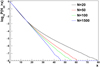 |
Fig. A.1. Logarithm of the H20 cumulative distribution for various data sample sizes. |
The asymptotic H20 probability distribution has been estimated using Monte Carlo (MC) by de Jager et al. (1989) and de Jager & Büsching (2010). It corresponds to a simple exponential P(H20 > x) = e−λx with λ ∼ 0.4. This result is very close to the analytic solution found by Kerr (2011) that yields a practical formula (valid for m ≥ 10) with λ = 0.398405.
Pulsation searches very often require multiple trials corresponding to different event selections. Some of these can lead to small data samples. As a consequence it is important to estimate the H20 probability distribution for low N, the number of events used when computing H20. To do so, we ran 109 MC realizations for various N, assigning a random phase to each event. Figure A.1 shows the logarithm of the cumulative distribution, log10P(H20 > x), for N = 20, 50, 100 and 1500. The asymptotic behaviour is reached in N = 1500 case but the distribution of the other cases shows a clear departure from the pure exponential above x ∼ 20.
To characterize this departure, we fitted log10P(H20 > x) with a linear polynomial over the interval corresponding to −7 < log10P(H20 > x) < − 4 (i.e. x ≳ 23). The slope λ1 of this linear polynomial is shown in Fig. A.2 as a function of N. We find the following parameterization for λ1 (shown in Fig. A.2):
 (A.1)
(A.1)
where λ0 = −0.398405/log(10)= − 0.173025.
We first approximate log10P(H20 > x) with a broken linear polynomial whose slopes at small and large x are λ0 and λ1(N), respectively. We find that the break position is compatible with x = 22 for all N. For low values of N the broken linear polynomial approximation does not work well around the break position, as shown in Fig. A.3. To have a better representation of log10P(H20 > x), we used a double broken linear polynomial approximation, with the same slopes at small and large x as for the single one, with break positions at x = 15 and x = 29:
 (A.2)
(A.2)
When considering the x interval such that P(H20 > x) > 10−7, the maximum of the absolute difference between the parameterization and the MC result is less than 0.1 for N ≥ 20. For N = 10, the maximum difference reaches 0.25 at x = 29. As a consequence, the approximation given by Eq. (A.2) is valid for N ≥ 20 with a 0.1 precision for P(H20 > x) > 10−7.
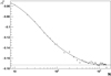 |
Fig. A.2. Parameterization of λ1, the slope of log10P(H20 > x) over the interval corresponding to −7 < log10P(H20 > x) < − 4, as a function of N. |
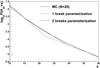 |
Fig. A.3. Logarithm of the H20 cumulative distribution for N = 20 in the x range where a single broken linear polynomial does not provide a good approximation. The black line corresponds to the MC result while the red and blue curves correspond to the single and double broken linear polynomial approximations, respectively. |
Appendix B: Monte Carlo estimated probability distribution of H20w
To estimate the probability distribution of H20w, we ran 108 MC realizations of a five-degree region of interest with a uniform background following the Galactic diffuse emission spectrum defined in Sect. 3.1 (corresponding to a broken power law, with spectral indices of ∼1.6 and ∼2.5 below and above ∼3 GeV, respectively), convoluted with the Fermi/LAT effective area. These realizations are performed for various numbers of events. For each realization, we compute H20w using the simple weights definition of Eq. (13) with σpsf set to one degree independently of energy. For CPU efficiency’s sake, each realization is used twice, with μw set to 2.5 and 3, each choice leading to a value of H20w.
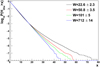 |
Fig. B.1. log10P(H20w > x) for various sum of weights. |
 |
Fig. B.2. Slope of log10P(H20w > x) over the interval corresponding to −7 < log10P(H20w > x) < − 4 as a function of W. Circles and triangles correspond to μw = 2.5 and 3, respectively. |
When parameterizing log10P(H20 > x) in the previous Section, we used the number of events because it drives the level of fluctuations. In the case of the weighted version of Htest, the number of events is not useful anymore. We used instead the sum of the weights, W, that we computed under the prescription that the maximum weight is one. Figure B.1 shows log10P(H20w > x) for some of the MC configurations corresponding to W ∼ 20, 50, 100, 700. As in the unweighted case, log10P(H20w > x) departs from a pure exponential at low W and can be approximated to first order by a broken linear polynomial. We note that the various MC configurations (number of events, μw choice) were chosen to explore a range for W between about 10 and 1000.
We estimate λ1, the slope over the interval corresponding to −7 < log10P(H20w > x) < − 4. Figure B.2 shows how the λ1 variation with W compares to the unweighted-case λ1 parameterization of Eq. (A.1). This parameterization works well for large values of W but not at low W. We find that using W + 5 instead of W gives a better match, as shown in Fig. B.3. The fact that increasing W leads to a better match is not surprising since, in the weighted case, the number of events that play a significant role in the H20w computation (i.e. with a relatively large weight) is on average larger than W.
 |
Fig. B.3. Slope of log10P(H20w > x) over the interval corresponding to −7 < log10P(H20w > x) < − 4 as a function of W + 5. Circles and triangles correspond to μw = 2.5 and 3, respectively. |
As a consequence, we used the following parameterization of log10P(H20w > x), that is obtained by simply replacing N by W + 5 in Eq. (A.2):
 (B.1)
(B.1)
When considering the x interval with P(H20w > x) > 10−7, the maximum of the absolute difference between the parameterization and the MC result is less than 0.1 for W ≥ 10. As a consequence, the approximation given by Eq. (B.1) is valid for W ≥ 10 with a 0.1 precision for P(H20w > x) > 10−7.
All Tables
Results of the TS < 25 pulsars: TS of the spectral fit, model and simple weight pulsation significances, Pm and Ps.
All Figures
|
Fig. 1. Weight position independent part f(E) for three test pulsar spectra. |
| In the text | |
|
Fig. 2. Pulsation significance as a function of μw for PSR J1646−4346. The upward arrows correspond to the first three trials, while the downward arrows correspond to the two subsequent trials. The sixth trial, shown with a circle, is the maximum of the Gaussian passing through the three points corresponding to the thick-line arrows. |
| In the text | |
|
Fig. 3. 68% width as a function of the peak position of Pw(μw) for the 144 pulsar sample. |
| In the text | |
|
Fig. 4. Pulsation significance in the (a, γ) parameter space normalized relative to its maximum for PSR J1646−4346. The dashed contour line corresponds to the 90% level. The solid straight line corresponds to the line Lm along which a scan is performed to obtain the model weight pulsation significance, as described in Sect. 4.4. |
| In the text | |
|
Fig. 5. Position of the lowest (dots) and highest (crosses) a points of ℰ90 (the region of the (a, γ) plane with Pw larger than 90% of the maximum) for the 144 pulsar sample. The solid line corresponds to the line Lm along which a scan is performed to obtain the model weight pulsation significance, as described in Sect. 4.4. |
| In the text | |
|
Fig. 6. Pulsation significance as a function of a, when scanning along Lm (solid line) and along LM (dashed line) for PSR J1646−4346. Lm and LM are two straight line in the pulsar parameter space (a, γ). Lm goes from (a = 0, γ = −1) to (a = 0.03, γ = 3) while LM approximates the ℰ90 major-axis. |
| In the text | |
|
Fig. 7. Correlation between γ0, the intercept of the ℰ90 major axis with the a = 0 axis, and am, the position of the maximum Pw along Lm for the 144 pulsar sample. The solid line shows the γ0 = 0.4 + 100am parameterization. |
| In the text | |
|
Fig. 8. Maximum Pw gain along LM as a function of its relative position with respect to am for the 144 pulsar sample. |
| In the text | |
|
Fig. 9. Model weight pulsation significance Pm as a function of TS for the 144 pulsar sample. Pulsation is detected for all pulsars, including the pulsars with TS < 25, whose results are reported in Table 1. |
| In the text | |
|
Fig. 10. Comparison of the model weight pulsation significance, Pm, and the pulsation significance derived when using the pulsar spectrum given by the spectral fit, Pfit, as a function of TS for the 131 pulsars with TS > 25 out of the 144 pulsar sample. The two methods give on average the same result but the model weight method is more sensitive by at least 20% for eight pulsars, whose results are reported in Table 2. |
| In the text | |
|
Fig. 11. Comparison of the model weight pulsation significance, Pm, and the pulsation significance derived when using the pulsar spectrum given by the spectral fit, Pfit, as a function of the “soft–and–flat” estimator Sf for the 131 pulsars with TS > 25 out of the 144 pulsar sample. The eight pulsars with Pm/Pfit > 1.2 are among the pulsars with the largest Sf, meaning those with the softest and flattest spectrum. |
| In the text | |
|
Fig. 12. Comparison of the pulsation significance obtained with an unweighted approach, Pgrid, and the model weight pulsation significance, Pm, as a function of TS for the 144 pulsar sample. The improvement of the model weight method over the unweighted approach is large, especially for the lowest TS pulsars. |
| In the text | |
|
Fig. 13. Comparison of the simple and model weight pulsation significances as a function of TS for the 144 pulsar sample. The simple weight method is on average ∼15% less sensitive than the model weight method. |
| In the text | |
|
Fig. 14. Average (solid) and lowest (dashed) ratio r(σw) over the 144 pulsar sample as a function of σw. For each σw, r(σw) is the ratio of Ps divided by the maximum Ps reached over the σw scan. |
| In the text | |
|
Fig. 15. Ratio of the pulsation significance with respect to Pm for the simple weights (solid), original event weight (dotted) and the grid search (dashed), for the 144 pulsar sample. |
| In the text | |
|
Fig. A.1. Logarithm of the H20 cumulative distribution for various data sample sizes. |
| In the text | |
|
Fig. A.2. Parameterization of λ1, the slope of log10P(H20 > x) over the interval corresponding to −7 < log10P(H20 > x) < − 4, as a function of N. |
| In the text | |
|
Fig. A.3. Logarithm of the H20 cumulative distribution for N = 20 in the x range where a single broken linear polynomial does not provide a good approximation. The black line corresponds to the MC result while the red and blue curves correspond to the single and double broken linear polynomial approximations, respectively. |
| In the text | |
|
Fig. B.1. log10P(H20w > x) for various sum of weights. |
| In the text | |
|
Fig. B.2. Slope of log10P(H20w > x) over the interval corresponding to −7 < log10P(H20w > x) < − 4 as a function of W. Circles and triangles correspond to μw = 2.5 and 3, respectively. |
| In the text | |
|
Fig. B.3. Slope of log10P(H20w > x) over the interval corresponding to −7 < log10P(H20w > x) < − 4 as a function of W + 5. Circles and triangles correspond to μw = 2.5 and 3, respectively. |
| In the text | |
Current usage metrics show cumulative count of Article Views (full-text article views including HTML views, PDF and ePub downloads, according to the available data) and Abstracts Views on Vision4Press platform.
Data correspond to usage on the plateform after 2015. The current usage metrics is available 48-96 hours after online publication and is updated daily on week days.
Initial download of the metrics may take a while.