| Issue |
A&A
Volume 622, February 2019
|
|
|---|---|---|
| Article Number | A158 | |
| Number of page(s) | 12 | |
| Section | Extragalactic astronomy | |
| DOI | https://doi.org/10.1051/0004-6361/201834519 | |
| Published online | 13 February 2019 | |
The magnetic field structure in CTA 102 from high-resolution mm-VLBI observations during the flaring state in 2016–2017
1
Max-Planck-Institut für Radioastronomie, Auf dem Hügel, 69, 53121 Bonn, Germany
e-mail: This email address is being protected from spambots. You need JavaScript enabled to view it.
2
Institute for Astrophysical Research, Boston University, Boston, MA 02215, USA
3
Astronomical Institute, St. Petersburg State University, St. Petersburg 199034, Russia
4
University of Crete, Heraklion, Greece
5
INAF – OAS Bologna, Area della Ricerca CNR, Via Gobetti 101, 40129 Bologna, Italy
6
Instituto de Astrofísica de Andalucía, CSIC, Apartado 3004, 18080 Granada, Spain
7
Korea Astronomy and Space Science Institute, 776 Daedeok-daero, Yuseong-gu, Daejeon 34055, Korea
8
Institut de Radio Astronomie Millimétrique, 300 Rue de la Piscine, 38406 Saint-Martin-d’Hères, France
9
Aalto University Metsähovi Radio Observatory, Metsähovintie 114, 02540 Kylmälä, Finland
Received:
26
October
2018
Accepted:
1
December
2018
Abstract
Context. Investigating the magnetic field structure in the innermost regions of relativistic jets is fundamental to understanding the crucial physical processes giving rise to jet formation, as well as to their extraordinary radiation output up to γ-ray energies.
Aims. We study the magnetic field structure of the quasar CTA 102 with 3 and 7 mm VLBI polarimetric observations, reaching an unprecedented resolution (∼50 μas). We also investigate the variability and physical processes occurring in the source during the observing period, which coincides with a very active state of the source over the entire electromagnetic spectrum.
Methods. We perform the Faraday rotation analysis using 3 and 7 mm data and we compare the obtained rotation measure (RM) map with the polarization evolution in 7 mm VLBA images. We study the kinematics and variability at 7 mm and infer the physical parameters associated with variability. From the analysis of γ-ray and X-ray data, we compute a minimum Doppler factor value required to explain the observed high-energy emission.
Results. Faraday rotation analysis shows a gradient in RM with a maximum value of ∼6 × 10⁴ rad m−2 and intrinsic electric vector position angles (EVPAs) oriented around the centroid of the core, suggesting the presence of large-scale helical magnetic fields. Such a magnetic field structure is also visible in 7 mm images when a new superluminal component is crossing the core region. The 7 mm EVPA orientation is different when the component is exiting the core or crossing a stationary feature at ∼0.1 mas. The interaction between the superluminal component and a recollimation shock at ∼0.1 mas could have triggered the multi-wavelength flares. The variability Doppler factor associated with such an interaction is large enough to explain the high-energy emission and the remarkable optical flare occurred very close in time.
Key words: instrumentation: interferometers / polarization / quasars: individual: CTA 102 / galaxies: active / galaxies: jets / instrumentation: high angular resolution
© ESO 2019
1. Introduction
Collimated outflows are launched from the centers of powerful active galactic nuclei (AGNs), and propagate at relativistic speeds often far beyond the host galaxy. Helical magnetic fields anchored in either the ergosphere of a spinning supermassive black hole (Blandford & Znajek 1977) or the accretion disk surrounding it (Blandford & Payne 1982; Zamaninasab et al. 2014) are thought to collimate and power these relativistic outflows. An observational signature of helical magnetic fields is a Faraday rotation gradient across the jet width due to the line-of-sight component of the magnetic field changing direction (e.g., Laing 1981).
One of the objects in which a large-scale rotation measure (RM) gradient has been observed is the flat-spectrum radio quasar (FSRQ) CTA 102. Hovatta et al. (2012) reported a significant transverse RM gradient at about 7 mas from the core region at 15 GHz. Hints that a helical magnetic field also exists in the innermost regions of the jets come from polarization observations at optical frequencies. The optical electric vector position angles (EVPAs) have been observed rotating in coincidence with a multi-wavelength flaring event that occurred in 2012 and that also coincided with the ejection of a new superluminal component from the radio core (Larionov et al. 2013; Casadio et al. 2015). Evidence for a physical connection between EVPA rotations and γ-ray flares has been found in a number of other sources (e.g., Marscher et al. 2010). This connection cannot be entirely attributed to a random walk process (Blinov et al. 2015). Therefore, it is important to observe sources during outbursts in order to study the correlated variability at the different frequencies as well as to investigate changes in polarized emission. Moreover, in many blazars, including CTA 102, γ-ray outbursts seem to be triggered by the passage of traveling component(s) through the radio core. If the radio core is a standing shock and the traveling component(s) is(are) a perturbation(s) in the jet flow, we expect the magnetic field parallel to the shock front to be amplified during the passage of each component through the core (Marscher & Gear 1985). This would also result in the reordering of the local magnetic field which in turn would produce an increase in the observed polarized radio emission.
We designed a monitoring program (PI: A. Marscher) consisting of Global millimeter(mm)-VLBI Array (GMVA) observations at 3 mm (86 GHz) of a sample of γ-ray bright blazars in support of the VLBA-BU-BLAZAR program1, which is a monthly monitoring with the VLBA at 7 mm (43 GHz) of 37 blazars and radio galaxies (e.g., Jorstad et al. 2017). The higher resolution (∼50 μas) and lower opacity at 86 GHz (in comparison to 43 GHz) allow us to probe deeper into the innermost regions of the jet and to investigate the structural changes and physical conditions within the jet also in connection with the γ-ray emission, which is thought to originate mainly in these regions. The GMVA observations are performed roughly every six months and the objects observed consist of the brightest sources (roughly half) of the VLBA-BU-BLAZAR sample (Jorstad et al. 2017).
In this paper we present results from the GMVA program obtained for the FSRQ CTA 102 (z = 1.037). The source recently underwent a prolonged active phase displaying, from the end of 2016 until beginning of 2017, a series of flares from the mm to the γ-ray energy band. A very bright flare occurred in the optical at the end of December 2016, when the source became the brightest blazar ever detected at these wavelengths. Coincident with this large optical flare were a series of outbursts that occurred closely in time across the γ-ray, X-ray, UV, and 1 mm radio bands (e.g., Raiteri et al. 2017; Kaur & Baliyan 2018).
The 86 and 43 GHz VLBI polarimetric data presented in this work cover the observing period from May 2016 to March 2017. The data set used for the analysis and the methods adopted for the data calibration are described in Sect. 2. In Sect. 3, we analyze the polarized emission at 86 and 43 GHz and in Sect. 4 we present our findings in connection with the multi-wavelength flares in 2016–2017. We adopt the cosmological values from the most recent Planck satellite results (Planck Collaboration XIII 2016): Ωm = 0.3, ΩΛ = 0.7, and H0 = 68 km s−1 Mpc−1. Assuming these values, and at the source redshift, 1 mas corresponds to a linear distance of 8.31 pc, and a proper motion of 1 mas yr−1 corresponds to an apparent speed of 55.2c.
2. Observations and data reduction
2.1. VLBI data analysis
The GMVA polarimetric data we present here were obtained on 21 May and 30 September 2016, and 31 March 2017. The antennas joining the GMVA array are: 8× VLBA stations (BR, FD, PT, LA, OV, KP, NL, MK), Green Bank Telescope (GB), Effelsberg (EB), Yebes (YS), Metsähovi (MH), Onsala (ON), Pico Veleta (PV), Plateau de Bure (PdB), and the Korean VLBI Network (KVN) array. In Table 1 we report the antennas for which it was possible to detect fringes, in each of the three observing sessions. Data are recorded at a rate of 2 Gbps (512 MHz bandwidth) in dual-polarization mode at all stations, aside from Yebes which records in single polarization. Afterwards, during the correlation process, data were split into eight 32 MHz sub-bands per polarization (IFs).
Antennas participating in GMVA sessions.
The a priori calibration (i.e., amplitude and phase calibration) of both 86 and 43 GHz data was performed following the usual procedure for high-frequency VLBI data reduction in Astronomical Image Processing System (AIPS); see for example Jorstad et al. (2017).
Since the expected atmospheric coherence time at 86 GHz is very short (∼10−20 s), the phase stability and the accuracy of the amplitude calibration are more critical than at longer wavelengths. As reported in Casadio et al. (2017), in order to check the reliability of the amplitude calibration, the final total flux density values have been compared with 3 mm single-dish measurements from the IRAM 30m antenna obtained under the POLAMI program2. In Table 2 we report the comparison of GMVA total flux densities and POLAMI (3 mm) single dish measurements of near-in-time epochs. We notice that the GMVA flux is lower than the POLAMI measurement in all the three epochs. Since CTA 102 is a relatively compact source, we expected a better match between the two measurements; it is therefore possible that the mm-VLBI total flux is slightly underestimated. However, as our study is mainly focused on the analysis of the polarized emission of CTA 102, these differences in flux density do not have an appreciable effect on the results of our study. We also use the POLAMI program measurements for the calibration of the absolute EVPA orientation, with uncertainties in the EVPAs ≤ 5° (Agudo et al. 2018a,b).
Single dish comparison.
The calibration of instrumental polarization is another complex step of polarimetric data reduction. After the a priori calibration, the data are transferred into Difmap to obtain the first total intensity image through a combination of CLEAN and self calibration. Afterwards, data are brought back to AIPS for the polarization calibration which consists of correcting for the instrumental polarization (D-terms) and the EVPAs absolute orientation. We tested two different methods for the calibration of instrumental polarization and used the most reliable one for the final calibration as described in Appendix A.
To carry out an analysis of the jet kinematics and flux density variability, we fitted the visibilities in Difmap with circular Gaussian components describing the brightness distribution. For each model-fit component, both at 3 and 7 mm, we obtain the flux density and position and we infer the relative uncertainties using the empirical relation in Casadio et al. (2015). Moreover, we added an additional 10%, coming from the typical amplitude calibration errors, and a minimum positional error of 0.005 mas, corresponding to ∼1/5 of the observing beam, (in quadrature) to the uncertainties above, as in Jorstad et al. (2017).
We calculate the uncertainties on the degree of linear polarization (σm) using the error propagation theory:
 (1)
(1)
 (2)
(2)
where σQ and σU are the rms noise of Stokes Q and U images,  is the linearly polarized flux density and I is the flux density in Stokes I, both with the respective uncertainties to which we added (in quadrature) a calibration uncertainty of 10% (Lico et al. 2014). To the σm obtained in Eq. (2) we add, in quadrature, σm, D, which is the feed calibration error we obtain from the analysis of the D-terms and is estimated using the following formula from Roberts et al. (1994):
 (3)
(3)
where σD is the standard deviation related to the weighted average D-term measurements (see Appendix A) and is of the order of 1–3%, Na is the number of antennas, NIF the number of IFs, and Ns is the number of sources we used to infer the weighted average D-terms data set. In the original formula (Roberts et al. 1994), Ns is the number of scans with independent parallactic angles, which in our case would be a larger quantity than the considered Ns, giving consequently even smaller σm, D. We obtained σm, D ≈ 0.1% and a final σm for the three epochs of between 0.4 and 0.7%. From the comparison of the different methods tested for the calibration of instrumental polarization in Appendix A, we notice that an imperfect D-term calibration could cause substantial changes in the polarized image and consequently in the degree of linear polarization. In contrast, the EVPA orientation was fairly constant with all the different methods; therefore for the EVPA errors we considered only the uncertainties of the POLAMI measurements.
2.2. X-ray and gamma-ray data analysis
For the acquisition of the γ-ray photon fluxes of CTA 102 we analyzed the publicly available Fermi Large Area Telescope (LAT) data (Atwood et al. 2009). Using the unbinned likelihood analysis of the Fermi analysis software package Science Tools v10r0p5 we processed the data in the 100 MeV ≤ E ≤ 100 GeV energy range. Within the 15° region of interest centered on the blazar we selected source class photons (evclass = 128 and evtype = 3). Photons with high satellite zenith angle (≥90°) were omitted in order to exclude the Earth limb background. The spatial model gll_iem_v06 was used to account for the diffuse emission from the Galaxy, while the isotropic spectral template iso_source_v05 was included in the fit for modeling of the extragalactic diffuse and residual instrumental backgrounds. We used P8R2_SOURCE_V6 as the instrument response function. In the background model we included all sources from the 3FGL (the third Fermi Gamma-ray catalog, Acero et al. 2015) located within 15° of the blazar. Spectral shapes of all targets except CTA 102 and photon fluxes of sources farther than 10° from the blazar were fixed to their values listed in the 3FGL. We used the test statistic value TS = 10 as the detection limit. This approximately corresponds to a 3σ detection level (Nolan 2012). The photon flux was integrated within six-hour time bins in order to maximize both the resolution of the light curve and the number of detections in it.
We collected X-ray data within the time range of interest from the Swift archive. The X-ray Telescope (XRT; Burrows et al. 2004) data were taken in the energy range 0.3–10 keV in Photon Counting mode and processed with the standard HEAsoft package version 6.19 in the manner described in Williamson et al. (2014). XSPEC software (Arnaud 1996) was used to fit the spectra by a single power-law model, with the neutral hydrogen column density equal to 5.04 × 1020 cm−2 (Dickey & Lockman 1990). We employed the Monte Carlo method in XSPEC to determine the goodness of the fit and uncertainties for each spectrum. The uncertainties of measurements are given at the 90% confidence level.
3. Polarization and rotation measure analysis
In Fig. 1 we display the three GMVA polarimetric images covering the period from May 2016 to March 2017. The source structure at 86 GHz in total intensity is relatively compact, while in linearly polarized intensity we can discern different features. In particular, it is interesting to notice the polarized emission downstream of the peak in total intensity, where the EVPAs have the same orientation as the jet direction for the May 2016 and March 2017 epochs. The maximum degree of polarization for the three epochs is comparable: between 8 and 14%.
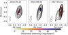 |
Fig. 1. 86 GHz GMVA polarimetric images of CTA 102. The restoring beams are 0.21 × 0.06, 0.26 × 0.06 and 0.25 × 0.05 mas, respectively. Total intensity peaks are 2.0, 1.77, and 3.79 Jy beam−1 and contours are drawn at 0.5, 0.85, 1.53, 3.02, 5.96, 11.74, 23.15, 45.65, and 90% of 3.79 Jy beam−1. |
In order to recover more polarized emission and lower the rms of the map, we also performed the stacking (average) of the three images in both total and linearly polarized intensity. For the linearly polarized intensity the stacking was done separately for the images of the Q and U Stokes parameters. The averaging in the image plane was performed after the alignment of the maps using the position of the peak in total intensity, which was coincident with the core position in all three epochs. Another method for the alignment of images makes use of the position of the VLBI core, which is determined through the modelfit procedure in Difmap package (e.g., Pushkarev et al. 2017). We compared both methods and found the first method to give better images (higher dynamic range) in the case of 86 GHz data. This could be a consequence of the higher angular resolution at 86 GHz, which causes the position of the core model-fit component to vary substantially among epochs.
In order to study the intrinsic magnetic field orientation we need to correct for the EVPA rotation introduced by the Faraday rotation. When the electromagnetic wave crosses a magnetized plasma, the polarization plane rotates due to a different propagation velocity of the left and right circularly polarized waves in which the linearly polarized radiation can be decomposed. The intrinsic polarization plane (χ0) is therefore rotated by a quantity, RM, which depends on the magnetic field (B) along our line of sight and the electron density (ne) of the intervening plasma:
 (4)
(4)
where e is the electron charge, ϵ0 the vacuum permittivity, m the electron mass, and c the speed of light. Given the linear dependence between the observed EVPAs and wavelength squared (λ2) in Eq. (4), the RM can be estimated from EVPA measurements at several frequencies.
We collected 43 GHz data from the VLBA-BU-BLAZAR program from June 2016 to April 2017, covering a time range similar to that covered by our GMVA epochs. The resulting polarimetric images were convolved with the same restoring beam (0.3 × 0.15 mas, 0°); we did the same for the GMVA images. The resultant 43 and 86 GHz images have been stacked using the method described above. The two stacked images at 43 and 86 GHz, displayed in Fig. 2, were used to obtain the RM image of CTA 102 between these two frequencies.
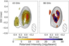 |
Fig. 2. 43 GHz VLBA (left panel) and 86 GMVA (right panel) stacked images. Black sticks represent EVPAs. The common restoring beam of 0.3 × 0.15 mas is displayed in the bottom-right corner. |
To obtain the RM image we first aligned the two images. Since the source is very compact at these frequencies, it was impossible to identify common optically thin regions. Therefore, we aligned the two stacked maps using a cross-correlation algorithm based on the correlation of total intensity images (e.g., Hovatta et al. 2012; Gómez et al. 2016). We obtained a shift to the southwest of 0.017 mas to align the 43 GHz image with respect to the 86 GHz one.
We also computed the spectral index (Sν ∝ να) map in order to check for optically thin/thick transitions in the core emitting region, where the EVPAs are expected to rotate by π/2 (Pacholczyk 1970). Figure 3 shows the spectral index map between 86 GHz GMVA and 43 GHz VLBA stacked images. Most of the core region is optically thick, becoming optically thin at ∼0.15 mas downstream from the core. Since the polarized emission is limited to the core region, which is mainly optically thick, we did not apply any rotation to EVPAs associated with opacity.
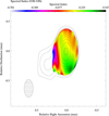 |
Fig. 3. Spectral index image between the 43 GHz VLBA and 86 GHz GMVA stacked images. Contours display the 43 GHz total intensity stacked map. The common restoring beam of 0.3 × 0.15 mas is displayed on the left. |
The RM map was obtained with the same approach described in Gómez et al. (2016). We made use of an IDL routine which estimates in each pixel the minimum RM value (i.e., the value that minimizes the nπ ambiguity in EVPAs). In Fig. 4 we present the resultant RM map.
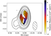 |
Fig. 4. Rotation measure image using the 43 and 86 GHz stacked images. Colors show the RM and black sticks the intrinsic (Faraday-corrected) EVPAs. The restoring beam and contours are the same as in Fig. 3. |
The Faraday rotation analysis between 43 and 86 GHz reveals RM values in the core region ranging from ∼−2 × 10⁴ to ∼6 × 10⁴ rad m−2, in agreement with values reported for this source in previous studies (Jorstad et al. 2007; Park et al. 2018). It also reveals a gradient around the centroid of the core and a change of sign, clearly visible from Fig. 4. The intrinsic EVPAs (i.e., the EVPAs corrected for Faraday rotation), represented by black sticks in Fig. 4, seem to rotate around the central peak.
The RM gradient, the change of sign, and the peculiar orientation of intrinsic EVPAs resemble the situation in BL Lacertae, as recently found by Gómez et al. (2016). The authors, who performed the Faraday rotation analysis using 15 and 43 GHz VLBA data and 22 GHz RadioAstron data, associate their findings to the presence of a large-scale helical magnetic field.
Relativistic magnetohydrodynamic (MHD) simulations including such large-scale helical magnetic fields in a Faraday rotating sheath surrounding the jet predict transverse gradient in RM (Broderick & McKinney 2010). In addition, the observed EVPA orientation around the core center has been produced by simulations in which the jet is observed at very small viewing angles (Porth et al. 2011). Hence we conclude that the core region in CTA 102 is threaded by a large-scale helical magnetic field.
4. The connection with the multi-wavelength flares in 2016–2017
4.1. The gamma-ray doppler factor
In Fig. 5 we show γ-ray (top panel) and X-ray (bottom panel) light curves, confirming the high state(s) of activity at both frequencies during December 2016–January 2017 (∼57735–57760 MJD). In both light curves we can separate two peaks: the first one around 57752 MJD (30 December) and the second 8 days later, around 57760 MJD.
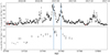 |
Fig. 5. Photon flux curves during the flaring period in γ-rays (top panel) and X-rays (bottom panel). The red triangles represent upper limits of the photon flux. |
Given the fact that we detect X-ray and γ-ray emission and the timing between the two frequencies suggests a common origin, we can use the method described in Mattox et al. (1993) to derive a lower limit for the Doppler factor (δγ). This method is based on the maximum optical depth allowed in order to avoid pair-production absorption, given a plasma moving relativistically as in AGN jets. We then inferred δγ for the two events using Eq. (4) in Mattox et al. (1993) and the parameters reported in Table 3.
Physical parameters used for deriving δmin from Eq. (4) in Mattox et al. (1993).
The variability timescales during the X-ray events in 57752 and 57760 MJD are ∼16 and 48 h, respectively, and these are the fastest significant variations we can derive from the X-ray light curve. Nevertheless these values could be underestimated, since a better sampling could give faster variability. The highest photon energy detected in the γ-rays during the flaring period is 364 GeV but since this value comes from only one photon we opted for a more conservative approach and used the value of 100 GeV, which is in agreement with the ∼98 GeV reported in Gasparyan et al. (2018).
For the two high-energy events we obtained δγ ≳ 17 during the first outburst (57752 MJD) and δγ ≳ 15 during the second (57760 MJD). Given the similarity of the two events in both the X-ray and γ-ray bands, similar limiting values for the Doppler factor were expected.
4.2. The Kinematics at 43 GHz and the variability Doppler factor
The model-fit analysis at 43 GHz allowed us to investigate the kinematics and flux density variability of the radio jet during the flaring period; see Figs. 6 and 7. We associated the core with the brightest unresolved component in the northwestern (upstream) end of the jet and we considered it to be stationary. Close to the core, at ∼0.1 mas, we detected another stationary component that we labeled C1, as we did in Casadio et al. (2015). Indeed, this stationary feature has already been observed in many previous studies (e.g., Jorstad et al. 2005, 2017), and was interpreted as a recollimation shock, which can trigger both radio (Fromm et al. 2013a) and γ-ray outbursts (Casadio et al. 2015). Another component, K0, is observed moving farther downstream in the jet.
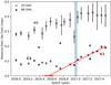 |
Fig. 6. Distance from the core vs. time of the 43 and 86 GHz model-fit components. The red line is the linear fit of K1 positions plus the uncertainty associated to the ejection time of the component. Blue vertical lines mark the time of the two high-energy events discussed in Sect. 4. |
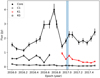 |
Fig. 7. Light curves of 43 GHz VLBA model-fit components. Blue vertical lines are the same as in Fig. 6. |
A new superluminal component, K1, has been visible in CTA 102 since November 2016 (see Fig. 6). From a linear fit of separation versus time we derived the velocity of K1, βapp = 11.5 ± 0.9c (0.209 ± 0.017 mas yr−1), and extrapolated the ejection time of the component (i.e., time of coincidence of the centroid of K1 with the centroid of the core), Tej = 2016.55 ± 0.07 (18 July 2016). Considering the average angular sizes of K1 and the core, which are a = 0.08 ± 0.01 mas and a0 = 0.025 ± 0.005 mas, respectively; the time K1 takes to exit the core is (a/2 + a0)/βapp = 114 days. This means that K1 starts exiting from the core on 2016.85 ± 0.04 (07 November 2016) and this coincides with a decrease in flux of the core which was previously in a flaring state; see Fig. 7.
Afterwards, at the beginning of 2017, both the light curves of K1 and the core show an increase in the flux density; the jet downstream, represented by K0, instead remains constant in flux. This increase in flux of K1 coincides with its passage through the stationary feature C1 and with the brightest phase of the flaring period at gamma and X-ray frequencies (see Fig. 5), but also at optical and UV frequencies (Raiteri et al. 2017; Gasparyan et al. 2018; Kaur & Baliyan 2018; Prince et al. 2018). After that, component K1 restarts its decreasing trend moving downstream along the jet while the core continues to vary around the flux of 2 Jy for many months.
In Fig. 6 we also show the position of the 86 GHz model-fit components in the three available epochs. Aside from the core we detect two more components, with the component closer to the core matching with the position of C1 in the first epoch, while in the last two epochs it seems to be co-spatial with the position of the new emerging component. With the few available GMVA epochs and the large separation in time, it is difficult to obtain an unambiguous match between components. However, with the identification of components as above, the new superluminal feature, K1, would be visible first at 86 GHz, in September 2016, and only later on at 43 GHz, as expected because of opacity effects.
Using the method in Jorstad et al. (2005) we estimate the Doppler factor associated with the flux variation observed in K1 when it crosses C1. The method relies on the comparison between the observed variability time scale, Δtvar, which is affected by the Doppler boosting, and the angular size of the component, which instead is not. The variability Doppler factor is hence derived as follows:
 (5)
(5)
where s = 1.6a and a = FWHM of the Gaussian component during the epoch of maximum flux, and DL is the luminosity distance. The variability timescale is defined as △tvar = dt/ln(Smax/Smin), where Smax and Smin are the measured maximum and minimum flux densities, respectively, and dt is the time in years between Smax and Smin. The only assumption here is that the variability time scale we observed corresponds to the light-travel time across the component. This occurs if the light crossing time is longer than the radiative cooling time and shorter than the adiabatic cooling time.
We wanted to test the hypothesis that the passage of K1 through the stationary feature C1 triggers particle acceleration and the multi-frequency outbursts in December 2016–January 2017. We infer the Doppler factor from both the rising and decaying time of the K1 flux density when it crosses C1. Hence, for measuring Smax, we considered the epoch of the peak in K1 when it is crossing the stationary feature (January 2017). Smin was measured in December 2016 and February 2017, respectively, for the rising and decaying variability time scale (see Fig. 7). The average variability Doppler factor we obtained considering the rising and decaying time of K1 crossing C1, is δvar = 34 ± 4.
Subsequently, combining the variability Doppler factor with the estimated apparent velocity (βapp) we also obtained the viewing angle and the Lorentz factor associated with the variation (see Jorstad et al. 2005 and Casadio et al. 2015 for the details). The values we obtained are θvar = 0.9 ± 0.2° and Γvar = 20.9 ± 1.9, respectively.
4.3. The polarized emission evolution at 43 GHz
In Fig. 8 we display a series of 43 GHz total and linearly polarized intensity images that are used for the Faraday rotation analysis presented in Sect. 3. The images cover the period of the K1 ejection and exit from the core, as well as the crossing time through C1. The new superluminal component K1 is ejected from the core during July 2016 and it takes until the beginning of November to cross the core region.
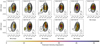 |
Fig. 8. 43 GHz VLBA polarimetric images of CTA 102. The common restoring beam is 0.15 × 0.3 mas. Total intensity peaks are 2.35, 2.39, 3.09, 3.59, 3.56, 2.07, 351, 2.64, 2.44, 1.86, and 1.89 Jy beam−1 and contours are drawn at 0.8, 1.53, 3.02, 5.96, 11.74, 23.15, 45.65, and 90% of 3.59 Jy beam−1. Black sticks represent polarization vectors. |
What we observe from Fig. 8 is that from July 2016 until September 2016, when K1 was crossing the core region, the EVPA orientation resembles the orientation present in the stacked image at 43 GHz (Fig. 2) and partially also the intrinsic orientation obtained from the Faraday rotation analysis (Fig. 4). The EVPAs in Fig. 4 are slightly rotated after the correction for Faraday rotation. This tells us that during these two epochs we are observing the magnetic field structure in the inner jet which is highlighted by the passage of the superluminal component. In the following epoch, October 2016, the EVPAs are, in contrast, mainly oriented at 90° and there is a peak in the polarized flux. We interpret this polarization morphology as a signature of the component K1 crossing the last optically thick surface of the core region and in turn highlighting the magnetic field structure present within this region of the jet. Subsequently, November 2016, the component is already outside the core and the EVPAs remain partially horizontal, mainly in the region where the component is moving.
Later, we observe another peak in polarization in January and this time the EVPAs are mainly oriented at 0°. This is the epoch of the passage of K1 through C1 with K1 increasing its flux density. The fact that EVPAs here are oriented at 90° with respect to their orientation in October 2016, and that C1 is still inside the 43 GHz beam, may suggests that the polarization vectors here are marking the magnetic field orientation in the stationary feature C1.
However, we cannot discard the possibility that the polarized emission of this epoch is still associated with the core, which is also in a renewed high state of flux. A rotation of 90° is expected because of opacity effects (Pacholczyk 1970) or even because of changes of the jet orientation with respect to our line of sight (Lyutikov & Kravchenko 2017). In both cases, however, a strong decrease of the degree of polarization is expected. Comparing the total intensity peaks and the polarized fluxes in the images of Fig. 8 we found no such decrease, leading us to discard both the aforementioned scenarios.
5. Discussion
In Sect. 3 we presented the Faraday rotation analysis between 43 GHz VLBA and 86 GHz GMVA data, which reveals a RM gradient with a maximum value of ∼6 × 10⁴ rad m−2 and a change of sign with position angle around the centroid of the core. The intrinsic EVPAs are observed rotating around the core. The RM gradient and EVPA orientation point to the presence of large-scale helical magnetic fields and a very small viewing angle (Broderick & McKinney 2010; Porth et al. 2011). This is also in agreement with the inferred viewing angle θvar = 0.9 ± 0.2°, obtained in Sect. 4. Considering this viewing angle and the projected distance of 3.86 × 10³ gravitational radii between the 86 GHz core and the black hole found in Fromm et al. (2015), we infer that the 86 GHz core is located at a de-projected distance of ∼2.5 × 10⁵ gravitational radii. Moreover, if we take into account the distance of ∼0.2 mas between the 15 and 86 GHz core regions reported in Fromm et al. (2015), the ∼7 mas distance from the 15 GHz core where Hovatta et al. (2012) detected a significant RM gradient across the jet translates into ∼3.9 × 10⁷ gravitational radii. We demonstrate the existence of a helical magnetic field all the way from ∼2.5 × 10⁵ to ∼3.9 × 10⁷ gravitational radii.
The RM analysis is performed during a very active state of the source. Multi-wavelength flares are detected from December 2016 to January 2017. From our γ-ray and X-ray analysis we distinguish two main outbursts which occurred very close to one another in time (December 30 and January 07). Optical and UV flares were also detected very close in time to the high-energy flares (Kaur & Baliyan 2018). The timing between the X-ray and γ-ray events suggests a common emitting region and this assumption allows us to infer a lower limit for the Doppler factor, δγ ≳ 15−17, needed to produce the observed high-energy emission.
From the 43 GHz kinematics analysis we find that a new superluminal component, K1, was ejected in July 2016 and moved downstream in the jet with an apparent speed of βapp = 11.5 ± 0.9c. The appearance of the component emerging from the core was accompanied by a decrease in the core flux density with the K1 light curve following a mainly decreasing trend attributable to adiabatic losses while the component propagates along the jet (Fromm et al. 2013b). However, this trend is interrupted by an increase in flux in January 2017, when the component K1 crosses a stationary feature (C1) which is located at ∼0.1 mas from the core. There is ample evidence (Jorstad et al. 2005, 2017; Fromm et al. 2013a,b; Casadio et al. 2015) that C1 is most likely associated with a standing recollimation shock in the jet.
The passage of K1 through the recollimation shock at 0.1 mas coincides with the flaring periods in the γ-ray, X-ray, UV, and optical pass bands. The Doppler factor that we deduce from the apparent velocity of K1 is around 11, but such a low value would not explain the observed high-energy emission, being incompatible with the lower limit for the Doppler factor we obtained in Sect. 4. If instead we infer the variability Doppler factor when the component K1 is crossing C1, we obtain a larger value: δvar = 34 ± 4. This value would explain the high-energy events and is also in agreement with the value found to explain the remarkable optical flare which occurred very close in time, on 28 December 2016 (Raiteri et al. 2017). Moreover, a similar variability Doppler factor for CTA 102 is reported in Casadio et al. (2015) and Jorstad et al. (2017). In Casadio et al. (2015) we found that a component with similar apparent speed (βapp = 11.3 ± 1.2c), slower than other previous components, was responsible for triggering an extraordinary multi-wavelength flare in 2012. The variability Doppler factor and viewing angle we inferred in that case were δ ∼ 30 and θ ∼ 1.2°.
The very small viewing angle obtained for K1 (θvar = 0.9 ± 0.2°) would explain the slowness of the component. We are not able to distinguish properly the motion of something moving toward us and this is the reason why the variability Doppler factor is more reliable than what we infer from the kinematics in these cases.
In Sect. 4 we have also compared the motion of K1 along the jet with the evolution of the 43 GHz linearly polarized emission. During the passage of the component through the core region the polarization vector orientation resembles the intrinsic orientation obtained from the Faraday rotation analysis. In contrast, a different EVPA orientation is observed when the component is almost exiting the core (EVPAs mainly at 90°) and crossing the stationary feature C1 (EVPAs mainly at 0°). We hypothesise that this evolution in the orientation of the EVPAs may be attributed to the component highlighting the magnetic field structure within two distinct regions of the jet. The different orientation of the EVPAs, shown when the component K1 is crossing the last optically thick surface in the core region and when it crosses C1, could be evidence of a distinct magnetic field orientation in the two regions. We plan to investigate this scenario, comparing our observations with RMHD simulations in a forthcoming publication. A 90° flip in the EVPAs due to opacity effects or different viewing angles is a less probable explanation considering the absence of an observed decrease in the level of fractional linear polarization.
6. Conclusions
We present mm-VLBI polarimetric images of the FSRQ CTA 102 with the highest possible resolution currently achievable (∼50 μas). The images were obtained with the GMVA at 86 GHz in May 2016, September 2016, and March 2017. Combining 43 GHz VLBA observations from the VLBA-BU-BLAZAR program with our 86 GHz GMVA data, we obtained the first high-resolution Faraday rotation image between these two frequencies. The Faraday rotation structure and the intrinsic EVPA orientation highlighted by the high-resolution image reveal the existence of a large-scale helical magnetic field in the very inner regions (∼2.46 × 10⁵ gravitational radii, deprojected) of CTA 102 jet.
From late 2016 to the beginning of 2017, CTA 102 was in a very active state, displaying extraordinary flares from radio to γ-ray frequencies. From the kinematics analysis at 43 GHz, we found that a new superluminal component was ejected from the mm core in July 2016. During the multi-wavelength outbursts, the new component was crossing another stationary feature located very close to the core (∼0.1 mas), increasing its flux density. This supports the nature of recollimation shock of the stationary feature at ∼0.1 mas and the expected particle acceleration during shock-shock interaction. In our scenario, the interaction between the moving component and the recollimation shock triggers the multi-wavelength flares from December 2016 to January 2017. This is also supported by the variability Doppler factor associated with such an interaction (δvar = 34 ± 4), which is enough to explain the brightest γ-ray and X-ray flares observed in that period as well as the increase of 6–7 magnitudes in optical on 28 December 2016 (Raiteri et al. 2017).
Acknowledgments
This research has made use of data obtained with the Global Millimeter VLBI Array (GMVA), which consists of telescopes operated by the MPIfR, IRAM, Onsala, Metsahovi, Yebes and the VLBA. The data were correlated at the correlator of the MPIfR in Bonn, Germany. The VLBA is an instrument of the National Radio Astronomy Observatory, a facility of the National Science Foundation of the USA operated under cooperative agreement by Associated Universities, Inc. (USA). The research at Boston University is supported by the NASA Fermi GI grant 80NSSC17K0649. Figure A.2 also appears in Casadio et al. (2017), published by Galaxies (an open access journal). We would like to thank the MPIfR internal referee Rocco Lico for the careful reading of the manuscript. We would also like to thank Helge Rottmann, Pablo de Vicente, Salvador Sanchez, Uwe Bach, Michael Lindqvist, and Jun Yang for the valuable GMVA data acquisition work. This paper is partly based on observations carried out with the IRAM 30 m Telescope. IRAM is supported by INSU/CNRS (France), MPG (Germany) and IGN (Spain). DB acknowledges support from the European Research Council (ERC) under the European Union’s Horizon 2020 research and innovation programme under grant agreement No 771282. IA acknowledges support by a Ramón y Cajal grant of the Ministerio de Ciencia, Innovación y Universidades (MICINU) of Spain. The research at the IAA-CSIC was supported in part by the MICINU through grant AYA2016-80889-P.
References
- Acero, F., Ackermann, M., Ajello, M., et al. 2015, ApJS, 218, 23 [Google Scholar]
- Agudo, I., Thum, C., Molina, S. N., et al. 2018a, MNRAS, 474, 1427 [NASA ADS] [CrossRef] [Google Scholar]
- Agudo, I., Thum, C., Ramakrishnan, V., et al. 2018b, MNRAS, 473, 1850 [NASA ADS] [CrossRef] [Google Scholar]
- Arnaud, K. A. 1996, in Astronomical Data Analysis Software and Systems V, eds. G. H. Jacoby, & J. Barnes, ASP Conf. Ser., 101, 17 [NASA ADS] [Google Scholar]
- Atwood, W. B., Abdo, A. A., Ackermann, M., et al. 2009, ApJ, 697, 1071 [NASA ADS] [CrossRef] [Google Scholar]
- Blandford, R. D., & Payne, D. G. 1982, MNRAS, 199, 883 [NASA ADS] [CrossRef] [Google Scholar]
- Blandford, R. D., & Znajek, R. L. 1977, MNRAS, 179, 433 [NASA ADS] [CrossRef] [Google Scholar]
- Blinov, D., Pavlidou, V., Papadakis, I., et al. 2015, MNRAS, 453, 1669 [NASA ADS] [CrossRef] [Google Scholar]
- Broderick, A. E., & McKinney, J. C. 2010, ApJ, 725, 750 [NASA ADS] [CrossRef] [Google Scholar]
- Burrows, D. N., Hill, J. E., Nousek, J. A., et al. 2004, in X-Ray and Gamma-Ray Instrumentation for Astronomy XIII, eds. K. A. Flanagan, & O. H. W. Siegmund, Proc. SPIE, 5165, 201 [NASA ADS] [CrossRef] [Google Scholar]
- Casadio, C., Gómez, J. L., Jorstad, S. G., et al. 2015, ApJ, 813, 51 [NASA ADS] [CrossRef] [Google Scholar]
- Casadio, C., Krichbaum, T., Marscher, A., et al. 2017, Galaxies, 5, 67 [NASA ADS] [CrossRef] [Google Scholar]
- Dickey, J. M., & Lockman, F. J. 1990, ARA&A, 28, 215 [NASA ADS] [CrossRef] [MathSciNet] [Google Scholar]
- Fromm, C. M., Ros, E., Perucho, M., et al. 2013a, A&A, 551, A32 [NASA ADS] [CrossRef] [EDP Sciences] [Google Scholar]
- Fromm, C. M., Ros, E., Perucho, M., et al. 2013b, A&A, 557, A105 [NASA ADS] [CrossRef] [EDP Sciences] [Google Scholar]
- Fromm, C. M., Perucho, M., Ros, E., Savolainen, T., & Zensus, J. A. 2015, A&A, 576, A43 [NASA ADS] [CrossRef] [EDP Sciences] [Google Scholar]
- Gasparyan, S., Sahakyan, N., Baghmanyan, V., & Zargaryan, D. 2018, ApJ, 863, 114 [NASA ADS] [CrossRef] [Google Scholar]
- Gómez, J. L., Lobanov, A. P., Bruni, G., et al. 2016, ApJ, 817, 96 [NASA ADS] [CrossRef] [Google Scholar]
- Gómez, J. L., Marscher, A. P., Alberdi, A., Jorstad, S. G., & Agudo, I. 2002, VLBA Scientific Memo #30 [Google Scholar]
- Hovatta, T., Lister, M. L., Aller, M. F., et al. 2012, AJ, 144, 105 [NASA ADS] [CrossRef] [Google Scholar]
- Jorstad, S. G., Marscher, A. P., Lister, M. L., et al. 2005, AJ, 130, 1418 [NASA ADS] [CrossRef] [Google Scholar]
- Jorstad, S. G., Marscher, A. P., Stevens, J. A., et al. 2007, AJ, 134, 799 [NASA ADS] [CrossRef] [Google Scholar]
- Jorstad, S. G., Marscher, A. P., Morozova, D. A., et al. 2017, ApJ, 846, 98 [NASA ADS] [CrossRef] [Google Scholar]
- Kaur, N., & Baliyan, K. S. 2018, A&A, 617, A59 [NASA ADS] [CrossRef] [EDP Sciences] [Google Scholar]
- Laing, R. 1981, ApJ, 248, 87 [NASA ADS] [CrossRef] [Google Scholar]
- Larionov, V. M., Blinov, D. A., Jorstad, S. G., et al. 2013, Euro. Phys. J. Web Conf., 61, 4019 [CrossRef] [Google Scholar]
- Leppanen, K. J., Zensus, J. A., & Diamond, P. J. 1995, AJ, 110, 2479 [NASA ADS] [CrossRef] [Google Scholar]
- Lico, R., Giroletti, M., Orienti, M., et al. 2014, A&A, 571, A54 [NASA ADS] [CrossRef] [EDP Sciences] [Google Scholar]
- Lyutikov, M., & Kravchenko, E. V. 2017, MNRAS, 467, 3876 [NASA ADS] [CrossRef] [Google Scholar]
- Marscher, A. P., & Gear, W. K. 1985, ApJ, 298, 114 [NASA ADS] [CrossRef] [Google Scholar]
- Marscher, A. P., Jorstad, S. G., Larionov, V. M., et al. 2010, ApJ, 710, L126 [NASA ADS] [CrossRef] [Google Scholar]
- Martí-Vidal, I., Krichbaum, T. P., Marscher, A., et al. 2012, A&A, 542, A107 [NASA ADS] [CrossRef] [EDP Sciences] [Google Scholar]
- Mattox, J. R., Bertsch, D. L., Chiang, J., et al. 1993, ApJ, 410, 609 [NASA ADS] [CrossRef] [Google Scholar]
- Nolan, P. L., Abdo, A. A., Ackermann, M., et al. 2012, ApJS, 199, 31 [NASA ADS] [CrossRef] [Google Scholar]
- Pacholczyk, A. G. 1970, Radio Astrophysics. Nonthermal Processes in Galactic and Extragalactic Sources (San Francisco: Freeman) [Google Scholar]
- Park, J., Kam, M., Trippe, S., et al. 2018, ApJ, 860, 112 [NASA ADS] [CrossRef] [Google Scholar]
- Planck Collaboration XIII. 2016, A&A, 594, A13 [NASA ADS] [CrossRef] [EDP Sciences] [Google Scholar]
- Porth, O., Fendt, C., Meliani, Z., & Vaidya, B. 2011, ApJ, 737, 42 [Google Scholar]
- Prince, R., Raman, G., Hahn, J., Gupta, N., & Majumdar, P. 2018, ApJ, 866, 16 [NASA ADS] [CrossRef] [Google Scholar]
- Pushkarev, A. B., Kovalev, Y. Y., Lister, M. L., & Savolainen, T. 2017, MNRAS, 468, 4992 [NASA ADS] [CrossRef] [Google Scholar]
- Raiteri, C. M., Villata, M., Acosta-Pulido, J. A., et al. 2017, Nature, 552, 374 [NASA ADS] [CrossRef] [Google Scholar]
- Roberts, D. H., Wardle, J. F. C., & Brown, L. F. 1994, ApJ, 427, 718 [NASA ADS] [CrossRef] [PubMed] [Google Scholar]
- Williamson, K. E., Jorstad, S. G., Marscher, A. P., et al. 2014, ApJ, 789, 135 [NASA ADS] [CrossRef] [Google Scholar]
- Zamaninasab, M., Clausen-Brown, E., Savolainen, T., & Tchekhovskoy, A. 2014, Nature, 510, 126 [NASA ADS] [CrossRef] [PubMed] [Google Scholar]
Appendix A: D-terms calibration
In polarimetric VLBI observations the signal is recorded by two orthogonal feeds, right and left circular, or RCP and LCP. The signal recorded by each feed not only contains the information on the polarized signal coming from the source, but also part of the signal of the other receiver that “leaks” into it. The “leakages” or “D-terms” quantify the instrumental polarization which has to be removed from data before the final imaging. The D-terms depend only on the station hardware and they are expected to change slowly with time (Gómez et al. 2002). We used the task LPCAL in AIPS to estimate the D-terms for all the sources observed under the aforementioned GMVA monitoring program (PI: A. Marscher) in the three epochs presented in this study. The LPCAL also provides the real parallactic angle coverage of each antenna (i.e., considering the scans kept after the calibration process), and this is an important parameter for the accuracy of the polarization calibration (Leppanen et al. 1995). Hence, we expect to have the same D-terms for all the sources with a measurement accuracy that depends mostly on the parallactic angle coverage, and in part also on the complexity of the polarized source substructure.
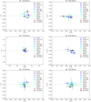 |
Fig. A.1. D-terms measurements obtained for all the sources observed in the 3 mm GMVA observation in March 2017 for FD, GB, and EB feeds. Red and black dots represent the weighted average values obtained for March 2017 and September 2016, respectively. |
In order to test the validity of D-term measurements, for each antenna feed (RCP and LCP) we compared the measurements coming from all the sources and we did this in all the three GMVA epochs, always taking LA as reference antenna. In Fig. A.1 we report, as example, the plots obtained for three antennas for the epoch of September 2016. The task LPCAL unfortunately does not provide any uncertainties on measurements; therefore we decided to use the parallactic angle coverage as weights for the relative comparisons between measurements. The D-terms magnitudes are in the range 1%–15%, in agreement with previous works Roberts et al. (1994), Martí-Vidal et al. (2012), but we also found some outliers, as for example 1633+382 in GB-LCP in September 2016 (see Fig. A.1), which we have not considered in our final analysis. Moreover, from the analysis of resulting plots we also decided to remove D-terms values with parallactic angle coverage below 70°. With the remaining measurements, we inferred weighted average values and the associated standard deviations for each feed and epoch. The standard deviations are around 1–3%.
The obtained average values for VLBA stations are not stable even on a six-monthly scale, contrary to what is reported in Gómez et al. (2002). The reason could be the 86 GHz receivers which do not provide stable D-terms or other hardware changes in VLBA stations. In any case, we cannot use the D-terms stability as a method for the calibration of the absolute orientations of EVPAs among epochs (Leppanen et al. 1995; Gómez et al. 2002).
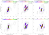 |
Fig. A.2. Series of 3 mm GMVA images in total (contours) and linearly polarized (colours) intensity of OJ 287, 1510–089, and CTA 102 taken on 21 May 2016. Black sticks represent the EVPAs. The images on top panel are obtained applying to the sources their own D-terms, while the bottom panel images result from the application of the average D-terms. |
We tested three different approaches for the calibration of the instrumental polarization. In the first epoch (May 2016) we chose three sources (OJ 287, 1510–089 and CTA 102) with different parallactic angle coverage and imaged each source using the D-terms obtained from its own data and the set of average D-terms obtained as described above. Figure A.2 displays the images of the three sources obtained applying both methods. In the case of OJ 287, which presents the best parallactic angle coverage (between 100° and 120° for most of the antennas), both methods give similar results; while for the other two sources, which have worse parallactic angle coverage (most of the antennas are below 95°) the resulting images present differences. The morphology of the polarized emission changes substantially between the two images, and the peak of the linearly polarized intensity shifts to a different position. Moreover, applying the average D-terms we obtained higher dynamic ranges in polarization confirming the influence of feed calibration errors in the dynamic range determination of the polarization images (Leppanen et al. 1995).
The third method consists in obtaining the D-terms of only one source, compact and with good parallactic angle coverage, and applying them to all the other sources. We tested this approach in the epoch of September 2016, using the D-terms of 0716+714 which is a compact source and in that epoch has a very good parallactic angle coverage in all the antennas. Figure A.3 displays the resulting images of 1510–089 and CTA 102 applying the D-terms of 0716+14 (top) and the average D-terms (bottom). Because of the good parallactic angle coverage of 0716+714, the images this time show no substantial difference, although applying the average D-terms we still have higher dynamic ranges.
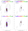 |
Fig. A.3. 3 mm GMVA polarimetric images of 1510–089 and CTA 102 in September 2016. Contours and colors represent the same as in Fig. A.2. The images on top panel are obtained applying the D-terms of 0716+714 and the bottom panel images applying the average D-terms. |
From the comparison of the three methods used for the calibration of the instrumental polarization, we decide to use the method of the average D-terms for all the sources and for the three GMVA epochs.
All Tables
Physical parameters used for deriving δmin from Eq. (4) in Mattox et al. (1993).
All Figures
|
Fig. 1. 86 GHz GMVA polarimetric images of CTA 102. The restoring beams are 0.21 × 0.06, 0.26 × 0.06 and 0.25 × 0.05 mas, respectively. Total intensity peaks are 2.0, 1.77, and 3.79 Jy beam−1 and contours are drawn at 0.5, 0.85, 1.53, 3.02, 5.96, 11.74, 23.15, 45.65, and 90% of 3.79 Jy beam−1. |
| In the text | |
|
Fig. 2. 43 GHz VLBA (left panel) and 86 GMVA (right panel) stacked images. Black sticks represent EVPAs. The common restoring beam of 0.3 × 0.15 mas is displayed in the bottom-right corner. |
| In the text | |
|
Fig. 3. Spectral index image between the 43 GHz VLBA and 86 GHz GMVA stacked images. Contours display the 43 GHz total intensity stacked map. The common restoring beam of 0.3 × 0.15 mas is displayed on the left. |
| In the text | |
|
Fig. 4. Rotation measure image using the 43 and 86 GHz stacked images. Colors show the RM and black sticks the intrinsic (Faraday-corrected) EVPAs. The restoring beam and contours are the same as in Fig. 3. |
| In the text | |
|
Fig. 5. Photon flux curves during the flaring period in γ-rays (top panel) and X-rays (bottom panel). The red triangles represent upper limits of the photon flux. |
| In the text | |
|
Fig. 6. Distance from the core vs. time of the 43 and 86 GHz model-fit components. The red line is the linear fit of K1 positions plus the uncertainty associated to the ejection time of the component. Blue vertical lines mark the time of the two high-energy events discussed in Sect. 4. |
| In the text | |
|
Fig. 7. Light curves of 43 GHz VLBA model-fit components. Blue vertical lines are the same as in Fig. 6. |
| In the text | |
|
Fig. 8. 43 GHz VLBA polarimetric images of CTA 102. The common restoring beam is 0.15 × 0.3 mas. Total intensity peaks are 2.35, 2.39, 3.09, 3.59, 3.56, 2.07, 351, 2.64, 2.44, 1.86, and 1.89 Jy beam−1 and contours are drawn at 0.8, 1.53, 3.02, 5.96, 11.74, 23.15, 45.65, and 90% of 3.59 Jy beam−1. Black sticks represent polarization vectors. |
| In the text | |
|
Fig. A.1. D-terms measurements obtained for all the sources observed in the 3 mm GMVA observation in March 2017 for FD, GB, and EB feeds. Red and black dots represent the weighted average values obtained for March 2017 and September 2016, respectively. |
| In the text | |
|
Fig. A.2. Series of 3 mm GMVA images in total (contours) and linearly polarized (colours) intensity of OJ 287, 1510–089, and CTA 102 taken on 21 May 2016. Black sticks represent the EVPAs. The images on top panel are obtained applying to the sources their own D-terms, while the bottom panel images result from the application of the average D-terms. |
| In the text | |
|
Fig. A.3. 3 mm GMVA polarimetric images of 1510–089 and CTA 102 in September 2016. Contours and colors represent the same as in Fig. A.2. The images on top panel are obtained applying the D-terms of 0716+714 and the bottom panel images applying the average D-terms. |
| In the text | |
Current usage metrics show cumulative count of Article Views (full-text article views including HTML views, PDF and ePub downloads, according to the available data) and Abstracts Views on Vision4Press platform.
Data correspond to usage on the plateform after 2015. The current usage metrics is available 48-96 hours after online publication and is updated daily on week days.
Initial download of the metrics may take a while.