| Issue |
A&A
Volume 622, February 2019
|
|
|---|---|---|
| Article Number | A112 | |
| Number of page(s) | 11 | |
| Section | The Sun | |
| DOI | https://doi.org/10.1051/0004-6361/201834283 | |
| Published online | 06 February 2019 | |
Link between trees of fragmenting granules and deep downflows in MHD simulation⋆
1
Institut de Recherche en Astrophysique et Planétologie, Université de Toulouse, CNRS, UPS, CNES, 14 Avenue Edouard Belin, 31400 Toulouse, France
e-mail: thierry.roudier@irap.omp.eu
2
Observatoire de Paris, LESIA, 5 Place Janssen, 92195 Meudon, France
3
PSL Research University, CNRS, Sorbonne Universités, UPMC Univ. Paris 06, Univ. Paris Diderot, Sorbonne Paris Cité, France
4
Physics and Astronomy Department, Michigan State University, East Lansing, MI 48824, USA
5
Lockheed Martin Solar and Astrophysics Laboratory, 3251 Hanover Street, Palo Alto, CA 94303, USA
Received:
19
September
2018
Accepted:
20
December
2018
Context. Trees of fragmenting granules (TFG) and associated flows are suspected to play a major role in the formation of the network in the quiet Sun. We investigate the counterparts, in terms of dynamics, of surface structures detectable by high resolution observations in deeper layers up to 15 Mm, which are only available from numerical simulations.
Aims. The first aim is to demonstrate that TFG can be evidenced either from surface intensitites, vertical (Vz), or Doppler (Vdop) velocities. The second is to show that horizontal flows, which are derived from intensities or Vz/Vdop flows, are in good agreement, and that this is the case for observations and numerical simulations. The third objective is to apply this new Vz-based method to a 3D simulation to probe relationships between horizontal surface flows, TFG, and deep vertical motions.
Methods. The TFG were detected after oscillation filtering of intensities or Vz/Vdop flows, using a segmentation and labelling technique. Surface horizontal flows were derived from local correlation tracking (LCT) and from intensities or Vz/Vdop flows. These methods were applied to Hinode observations, 2D surface results of a first simulation, and 3D Vz data of a second simulation.
Results. We find that TFG and horizontal surface flows (provided by the LCT) can be detected either from intensities or Vz/Vdop component, for high resolution observations and numerical simulations. We apply this method to a 3D run providing the Vz component in depth. This reveals a close relationship between surface TFG (5 Mm mesoscale) and vertical downflows 5 Mm below the surface. We suggest that the dynamics of TFG form larger scales (the 15–20 Mm supergranulation) associated with 15 Mm downflowing cells below the surface.
Conclusions. The TFG and associated surface flows seem to be essential to understanding the formation and evolution of the network at the meso and supergranular scale.
Key words: Sun: photosphere / Sun: granulation / Sun: interior
Movies associated to Figs. 3, 11, 12, and 14 are availabe at https://www.aanda.org
© ESO 2019
1. Introduction
Knowledge of the solar plasma and magnetic field dynamic evolution requires observation data at all spatial and temporal scales. Likewise, for a better description of the physical processes in the Sun, simulations need to integrate the smallest scales that are observable on the Sun into their global models. Currently, thanks to the capabilities of computers, these simulations are able to manage various scales (from granulation to supergranulation and larger scales). Nelson et al. (2018) have shown the importance of introducing simulations on scales up to the supergranulation to overcome the convection conundrum, which is related to the introduction of high resolution in global 3D simulations to describe correctly the Sun’s observed differential rotation and cyclic dynamo action. More particularly, Nelson et al. (2018) have imposed in their simulation small-scale convective plumes to mimic near-surface convective downflows (plumes) from supergranular flows. Moving inward, the plumes merge showing larger, more complex downflows. The introduction of these near-surface plumes then produces convective giant cells in the deeper layers through plume self-organization.
From the point of view of the observer, the determination of the flow organization on the solar surface and deeper inside the Sun (a few megametres) is still currently a challenge. Different approaches have been performed to improve the description of the convective-turbulent motions; these include helioseismology, correlation tracking, morphologic techniques such as network void or the detection the trees of fragmenting granules (TFG; Greer et al. 2016; Roudier et al. 2003, 2016; Berrilli et al. 2014; Rieutord & Rincon 2010). Using a new helioseismic technique Greer et al. (2016) showed that supergranulation probably forms at the surface, then rains downward imprinting its pattern in deeper layers. The slow upflows could be produced passively to fill the spaces between downflowing material. In that case, the upper convection zone is driven by the surface cooling (Greer et al. 2016).
The TFG detection is generally derived in the quiet Sun at disc centre from intensity observations with the Solar Optical Telescope (SOT on board Hinode; Roudier et al. 2016, 2003). However, Malherbe et al. (2018), using surface results of a 3D numerical simulation of the magneto-convection, showed that TFG also form in the emergent intensity of the simulation (at τ = 1) and are able to reproduce the main properties of solar TFG, such as lifetime and size, associated horizontal motions, corks, and diffusive index, close to observations. While TFG appear to structure the flows and magnetic field on the Sun surface (Malherbe et al. 2018; Roudier et al. 2016, 2003), we do not know the imprint of such a flow organization deeper in the Sun. In this paper, from a recent 3D numerical simulation of the magneto-convection, we use the vertical velocities Vz (z = 0.48 Mm to z = −20.3 Mm) to screen their link or not with the TFG detected on the surface. We use first 2D results (z = 0 Mm emergent intensity and surface velocity vector) of a 24 h sequence extracted from a longer 3D numerical simulation for testing TFG/LCT methods based on Vz detection and for comparison with Hinode observations. A second 4 h sequence of a 3D vertical velocity component (Vz only) is extracted from another 3D numerical simulation.
Section 2 describes the simulation data and the solar observation obtained with SOT/Hinode satellite. The detection of the TFG in the Vz component (equivalent to the solar radius direction) and horizontal velocity also measured by local correlation tracking (LCT) on the Vz component are described in Sect. 3. That TFG and the horizontal velocity are compared to those obtained in the emergent intensity at τ = 1 (Sect. 3). The TFG identified with Hinode data in the intensity and Doppler fields validate the detection on real solar data of same TFG in both methods (Sect. 4), where Vz of the simulation is replaced by the Doppler velocity. The links between TFG found in the Vz component, in the 4 h simulation, at the surface at τ = 1, the Vz velocities in depth (5, 15 Mm), and the correlation between the surface dynamics and deeper are described in Sect. 5. The results are summarized and discussed in the conclusion (Sect. 6).
2. Simulation data and Hinode solar observations
We used the 2014 results of the 3D magneto-convection code (Stein & Nordlund 1998; Stein et al. 2009, review by Stein 2012), which was not designed to model solar TFG. This code solves the equations of mass, momentum, and internal energy in conservative form plus the induction equation of the magnetic field for compressible flow on a staggered mesh. Boundaries are periodic horizontally and open at the top and bottom. Radiative heating/cooling is calculated by explicitly solving the radiation transfer equation in both continua and lines assuming LTE. The number of wavelengths for which the transfer equation is solved is reduced via a method which models the photospheric structure. Runs have dimensions 2016 × 2016 × 500 with resolution 48 km horizontally and 12–80 km vertically. Then the horizontal field is 96 Mm × 96 Mm and the vertical axis extends from the temperature minimum (0.48 Mm) down to 20.3 Mm below the visible surface.
Two data sets of magnetohydrodynamics (MHD) simulations, described above, were used to detect the TFG. The first is a 24 h duration sequence of the emergent intensity, surface vertical velocity (Vx,Vy,Vz), and magnetic field vector extracted between t = 59.6 h to 83.6 h and a field of 96 Mm × 96 Mm. Because of the huge volume of the data, we restricted the analysis to the field of 48 Mm × 48 Mm (65″ × 65″). For that sequence we have only intensity and velocity vector at τ = 1 (z = 0 Mm). Hence, horizontal plasma flow (Vx, Vy) can be compared to those detected by the LCT applied to intensity or Vz component alone. Because of the huge volume of the data the pixel was rebinned from 0.065″ to 0.13″ and the time step is 60 s. In order to be in the same condition as solar observations, both quantities (intensity and velocity) were filtered by the Hinode point spread function (PSF) at 557.6 nm. To remove the 5 min oscillations, we applied a subsonic Fourier filter in the k − ω space, where k and ω are the horizontal wave number and pulsation, respectively. All Fourier components such that ω ≤ Cs × k, where Cs = 6 km s−1 is the sound speed and k the horizontal wave number, were retained to keep only convective motions.
Because of the huge volume of data in the second MHD simulation of 4 h duration, we used only the vertical velocity Vz as a function of depth between z = 0.48 Mm (top) to z = −20.3 Mm (bottom) from t = 68.15 h to 72.25 h. The horizontal field is 96 Mm × 96 Mm. The other components (intensity, Vx, Vy and magnetic field) exist, but we were not able to get these owing to excessive data volume. Figure 1 shows the depth in Mm relatively to z pixels. Because of the large data volume the z pixel was rebinned by a factor 2, such that Vz at τ = 1 corresponds to the z pixel 20 and 242 to equates to a depth of −20 Mm. Again, owing to the large amount of data, the (x, y) pixel was rebinned from 0.065″ to 0.13″. The sequence time step is 60 s. For surface only (z = 0) the data were filtered by the Hinode PSF at 557.6 nm and then the 5 min oscillations were removed in the same way as described above for the previous simulation.
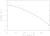 |
Fig. 1. Depth in Mm relatively to z pixels |
In order to compare TFG detected from solar observations in intensity and Doppler, we used Hinode NFI FeI 557.6 nm data, a 6 h sequence on 14 April 2010 from t = 7 h to 13 h UT That sequence represents 7000 spectral images with a pixel of 0.08″ rebinned to 0.16″. The time step is 28.75 s for 7 wavelengths (−12, −8, −4, 0, 4, 8, 12) pm, but the theoretical resolution of the Lyot filter is 6 pm. Scattered light of the filter was roughly corrected. Granulation intensity was derived from the average of wings at −12 and +12 pm at z close to the solar surface. Bright points were identified from core intensity at z = 180km above the surface (Malherbe et al. 2015). The Doppler shifts were computed with the bisector technique around inflexion points providing Vdop above the solar surface at z = 130km (Malherbe et al. 2015). Intensity and Vdop were recentred by cross correlation and filtered from 5 min oscillations. The FeI 557.6 nm line is insensitive to magnetic fields and the bright points observed in the intensity line correspond to hot spots that are considered as proxies of magnetic fields. No CaII H or magnetic data are available from Hinode for this observation. Figure 2 gives the magnetic context quiet Sun at the disc centre on 14 April 2010 (11 h UT) from a MDI longitudinal magnetic field observation.
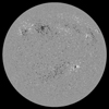 |
Fig. 2. Longitudinal magnetic field context from SOHO/MDI on 14 April 2010 (11 h UT) |
3. TFG and horizontal flows detected in Vz (0 Mm) of the long sequence (24 h) simulation
The first step of our analysis is to compare the TFG detected in the emergent intensity and Vz (radial velocity) on the 24 h simulation. Both sequences are filtered by the Hinode PSF. The TFG are detected using a segmentation and labelling technique described in detail by Roudier et al. (2003). Although we can recognize each granule in grey levels at the top of Fig. 3 where intensity and Vz are shown, the granules appear slightly different in amplitude repartition. This is why the transformation of the intensity and Vz maps into binary maps gives a relative different proportion of granule area to the total area of 41% and 38%, respectively. The bottom of Fig. 3 shows the TFG detected from intensity or Vz segmentation at the end of the sequence (24 h) with superimposed corks (white) which move freely at the speed of the horizontal flow (Vx, Vy) provided by the LCT (using classical 30 min and 3″ windows, left) or by the plasma velocity (right). We checked that cork final positions, based on the LCT or true plasma velocity of the simulation, are almost identical for the reasons described below. Most of TFG can be identified in both maps (intensity and Vz). The different temporal labelling is essentially due to the different amplitude repartition in granules of the intensity and velocity Vz component. In both maps corks are located on the edges of TFG and delineate supergranular scale. The temporal evolution of the TFG and corks is shown in the animation movie1 attached to Fig. 3 (bottom).
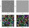 |
Fig. 3. Top panel: typical emergent intensity (left panel) and vertical velocity Vz (right panel) at the surface (z = 0 Mm) from the 24 h simulation. Bottom panel: TFG and corks (white crosses) detected from the emergent intensity at the end of the 24 h simulation (left panel); TFG detected from the velocity component Vz with corks derived from the horizontal plasma velocity Vx, Vy (right panel). The movie1.mp4 shows the temporal evolution of the bottom figures. The time step is 60 s; field of view (FOV) is 65″ × 65″. |
The correlation between the velocity obtained via the LCT, on both fields (intensity and Vz) gives a coefficient of 98%. Figure 4 shows the angular gap and ratio repartition between the two LCT velocity measurements giving the maximum error on the angle and module determination: ±5° in 50% and ±16° in 90% of the cases, and 9% in 50% and 29% in 90% of the cases on the module. These values indicate a very good correspondence between the horizontal velocities measured with LCT on intensity and Vz fields. Figure 5 exhibits the comparison of the simulation plasma horizontal velocity with velocity measured by LCT on the intensity and Vz fields. In that case the distributions are larger due to, in large part, the spatial and temporal averaging windows used in the LCT velocity determination.
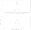 |
Fig. 4. Angular gap and ratio of velocities obtained with LCT (windows 30 min. and 3″) on emergent intensity to Vz components. |
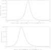 |
Fig. 5. Comparison between velocities of the plasma and velocities obtained with LCT on emergent intensity (solid line) and comparison between plasma velocities and velocities obtained with LCT on Vz (dotted line). The LCT windows 30 min and 3″ 24 h statistics. Top panel: angular shift between velocity vectors. Bottom: ratio between velocity vector modules. |
Figure 6 shows the similarity of the histogram of the TFG lifetimes for emergent intensity and velocity Vz. That distribution function of family lifetimes is typically a power law which is in good agreement with previous results (Malherbe et al. 2018). The comparison in Fig. 7 of the histograms of TFG maximum area during their lifetimes exhibits a small difference in the area that is smaller in size owing to the lower proportion of granule area in the Vz component; however, for the larger areas the behaviour is very similar.
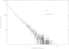 |
Fig. 6. Lifetime histograms of TFG detected from Vz (τ = 1 (at 0 Mm)) and emergent intensity. |
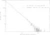 |
Fig. 7. Size histograms of TFG detected from Vz (τ = 1 (at 0 Mm)) and emergent intensity. |
4. Hinode TFG and horizontal flows detected in Doppler and intensity
Our goal is to detect TFG on emergent intensity and Doppler velocities on real solar data to compare to the previous results obtained with the simulation, where now the Vz of the simulation is replaced by the Doppler velocity (Vdop). From spectral images observed by Hinode, we can build temporal sequences in intensity and Dopplergram. The Doppler is deduced from the observed line profile while the Vz plasma velocity is computed for each altitude of the simulation. So the Dopplergrams reflect, at the disc centre, the radial velocities in a range of altitudes with a maximum of the contribution function around 130 km (Malherbe et al. 2015; Sheminova 1998). Figure 8 (top) shows intensity and Dopplergram at the end of the sequence and reveals the difference of appearances of both fields. This reflects the different altitudes of formation (intensity in line wings, dopplershifts at inflexion points), integration along the line of sight, which is also degraded by stray light and limited spectral resolution of the NFI filter. However, the solar granules are identifiable in both fields. As for the simulation sequences, the transformation of the intensity and Vdop maps into binary maps gives a different relative proportion of granule area to the total area of 38% and 37%, respectively. Figure 8 (bottom) shows the TFG detected for both components (intensity, Doppler) at the end of the sequence (6 h) and can be identified in both maps. The different temporal labelling is essentially from the different amplitude repartition in granules linked to the altitude of formation and integration.
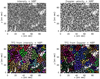 |
Fig. 8. Top panel: Hinode observation with NBPs at line centre superimposed (white). Intensity (left panel) and Doppler velocity (right panel). Bottom panel: TFG with NBPs superimposed (white). TFG derived from intensities (left panel) and TFG derived from Doppler shifts (right). |
Figure 9 shows the 6 h averaged module of the horizontal velocities Vh derived from LCT (classical windows 30 min, 3″) applied on intensity and VDop fields. The Vh fields measured on intensity and Doppler maps are similar in amplitude and repartition. The bright points detected in the central part of the line 557.6 nm used as proxy of the longitudinal magnetic component are located in lowest amplitude of the horizontal velocities forming aligned structures which delineate a supergranule in the central part of the figures. Figure 10 shows the TFG detected from the intensity and Vdop with final positions of corks superimposed (white crosses). Corks delineate the TFG at the meso or supergranular scale and are located close to the proxies of the magnetic field, network bright points (NBPs; see Fig. 8). The spatial correspondence between corks and the proxy of the magnetic field indicates a good determination of the flow field also related to the TFG evolution.
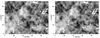 |
Fig. 9. Six hour averaged module of the horizontal velocities Vh computed with LCT (windows 30 min, 3″) on intensity (left panel) and Doppler velocity (right panel) with NBPs (line centre) superimposed (white). |
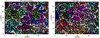 |
Fig. 10. TFG detected from the intensity and Doppler field with corks superimposed (in white). |
5. Surface TFG and deep downdraft predicted by the (4h) 3D simulation of vertical velocity Vz
The 4 h simulation of the vertical velocity Vz (Fig. 11) allows us, for the first time, to study the link between surface properties and downflows from depth between z = 0.48 Mm (top) to z = −20.3 Mm (bottom). The vertical velocity Vz from the top to the bottom is shown in the animation movie2 attached to Fig. 11. The downflows at different depths (z = 0, −5, −15 Mm) with superimposed corks in black (evolution described below) are shown in the animation movie3 attached to Fig. 12. That movies immediately reveal the existence of three downflowing scales: intergranules (blue), the mesoscale (green) and the supergranulation scale (red). At the bottom of our data cube, the larger scales are visible because downflows are collected and mixed to form a larger structure with depth.
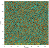 |
Fig. 11. Vz of the simulation at the altitude z = 0 Mm. Green corresponds to the granule (upflows) and orange to intergranule (downflows). The movie2.mp4 shows the vertical velocity (orange/green = downward/upward) of the simulation at different depths from +0.5 Mm (above the surface) to −20 Mm (below the surface). FOV is 131″ × 131″. |
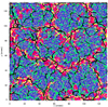 |
Fig. 12. Vz downflows visible at different depths of the simulation with superimposed corks (in black). Blue corresponds to z = 0 Mm (intergranules), green to z = −5 Mm (structures with TFG scale) at the same time, and red to z = −15 Mm where the supergranular scale (matching about 10 TFG) is observed. The movie3.mp4 shows the temporal evolution of that figure. Time step is 60 s; FOV 131″ × 131″. |
5.1. Corks and downdraft location with depth
The horizontal velocities obtained with LCT (windows 30 min and 3″) on the Vz component at the surface (0 Mm) allows us to compute the corks trajectories during the 4 h sequence. At the surface (z = 0 Mm) the corks diffused by the horizontal flows are located between TFG (Fig. 13) as previously observed (Roudier et al. 2016). At the end of the sequence, corks form a larger scale than TFG, which can be compared to the downflowing ribbons at 8 or 15 Mm. (see for comparison Fig. 14). This indicates the intimate link between the horizontal flow at the surface and the downflow network in the deeper layers.
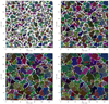 |
Fig. 13. Detected TFG on the 4 h Vz simulation at z = 0 Mm with corks superimposed (white) at different times as follows: 60, 80 (top panel), 120, and 240 (bottom panel) minutes. |
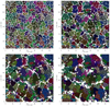 |
Fig. 14. TFG detected from the Vz component at z = 0 Mm with superimposed downflows (white) at different depths below the surface as follows: 3.0 Mm (top left panel), 5.0 Mm (top right), 8.0 Mm (bottom left panel), and 15 Mm (bottom right panel). movie4.mp4, movie5.mp4, movie6.mp4, and movie7.mp4 show the evolution of the families at the surface (z = 0) and the downflow (white) at different depths of 3.0, 5.0, 8.0, and 15.0 Mm below the surface, respectively. Time step is 60 s; FOV 131″ × 131″. |
5.2. TFG and downdraft location
First, we tried to detect correspondence between the location of large amplitude downdrafts visible at 0 Mm and at a depth of 20 Mm. The vertical location of the downdraft at 20 Mm depth corresponds in half of the case upflows at 0 Mm and vice versa between 0 Mm and 20 Mm. This indicates clearly that larger amplitude downdrafts observed at the surface do not reflect the downflow location in depth. This probably explains why heliosismology does not find coherence beyond 7 Mm and has difficulty detecting supergranules in depth. The second approach is to locate downflows at different depths relative to the TFG that structure flows at the surface (0 Mm).
The analysis of sequence (4 h) of the vertical velocity Vz as a function of depth between z = 0.48 Mm (top) to z = −20.3 Mm allows us to locate the TFG relative to the downflows. Figure 14 shows the TFG detected during 4 h at 0 Mm depth with superposed downflows at different depths of 3.0, 5.0, 8.0, and 15 Mm. The temporal evolutions at those different depths are shown in the animations movies 4, 5, 6, and 7 attached to Fig. 14. In the first depth of 3 Mm, no special link between TFG and downflows at the depth are visible. At 5 Mm depth, we clearly observe the downflows at the limit of the TFG indicating a connection of that flow and the granule evolution at 0 Mm. For deeper depth (8.0, 15.0 Mm) the downflows are still between TFG but include several of them. This is due to the limited duration of our sequence (4 h) where the TFG are not fully developed in size. We observe some of these as older branches of larger TFG. The spatial coherence due to families of granules at the surface sweeps the strongest movements, high horizontal velocities inside the TFG cells at z = 0 Mm, towards their boundaries where almost null horizontal velocity at z = 0 Mm corresponds to deep vertical flows (Roudier et al. 2016). This generates continuous descending motion, at meso and supergranular scales, which penetrate more deeply up to 20 Mm.
5.3. Module of the horizontal velocity and downdraft location
Figure 15 shows in greyscale the 4 h averaged horizontal velocity module (Vh) computed with LCT (using classical windows of 30 min and 3″) at 0 Mm on Vz component, with superposed downflows (white line) at different depths of 3.0, 5.0, 8.0, and 15 Mm. Almost null horizontal velocity regions (black) at z = 0 form ribbons corresponding to the large-scale downflows observed from 5 to 15 Mm. That also corresponds to the limits of the TFG (see Fig. 14) and indicates the link between TFG evolution at the surface and downdraft flows in the deeper layers of the 20 Mm box. In addition, the maxima of Vh amplitude (inside TFG but near boundaries) are observed close to the low Vh amplitude ribbons and also to the TFG borders (Roudier et al. 2016). If we now look at the dynamics of the downflows at 3 Mm depth, the second part of the moviesg (movie3 and movie4) reveals the proper motions of the downflows inside TFG to the limit of the TFG. Thereby the downflows are collected at the boundaries of the TFG, which also merge during their evolution. This process seems to generate structures on a larger scale which are linked to the downflows observed in depth of the simulation. This can be compared with the scenario described by Greer et al. (2016) in which the supergranulation appears to form at the surface and rains downward, imprinting its pattern in deeper layers. The analysis of our short simulation sequence (4 h) adds to this view the evolution of the TGFs (expansion, proper motions, mixing), which generates horizontal flows at the surface (0 Mm) whose action sweeps downflows at their borders. Thus we can draw a scenario where the collective effect of explosive granules, which form TFG, tend to form at their limits continuous descending motions that aggregate deeper on a larger scale downflow. The imprint on the surface motions can be observed at the border of TFG in the form of weak horizontal velocity amplitude but inside TFG, higher (and diverging) velocities are present. Table 1 summarizes the quantitative mean values (Velocities and divergence) measured on different locations and from corks motions.
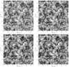 |
Fig. 15. Four hour averaged horizontal velocity (Vh) module at z = 0 Mm with superimposed downflows (white contours) at different depths below the surface: 3.0 Mm (top left), 5.0 Mm (top right panel), 8.0 Mm (bottom left panel), and 15 Mm (bottom right panel). |
Quantitative mean values measured on different locations at z = 0 Mm and from corks motions.
6. Conclusions
The main goal of our analysis was to demonstrate that TFG and horizontal velocities issued from LCT can be detected either in intensity or vertical velocity (Vz) field sequences, both in simulations or in disc centre observations (in that case, Doppler shifts replace the vertical velocity component). We checked that TFG and dynamics exhibit in surface results of a first simulation the same properties as those observed with Hinode. Using data of a second simulation providing Vz in depth, we studied TFG formation and evolution in relation with vertical flows below the surface, in unobservable layers.
From Hinode/NFI observations (disc centre), we found that TFG are detectable either in intensity or Doppler shifts and are very similar with both methods. As in previous works (Roudier et al. 2016, 2009; Roudier & Muller 2004) the magnetic field (in this case a proxy from NBPs) is located at the border of TFG. Horizontal velocity fields (from LCT) also play an important role because the slowest flows match the boudaries of TFG and form a supergranular scale.
The TFG detected in intensity and Vz velocity, in the surface results of the 24 h simulation, are also similar, indicating that both methods can be used. This is also the case for horizontal flows derived from LCT applied either to intensity or Vz, which are highly correlated.
The analysis of the 4 h simulation of the vertical velocity Vz as a function of depth between z = 0.48 Mm (top) to z = −20.3 Mm (bottom) reveals the intimate relation between the TFG detected at the surface at z = 0 (on the Vz component) and deeper downflows.
In the first megametres depth, we observe no special link between TFG and downflows. At 5 Mm depth, downflows are clearly located below the boundaries of the TFG. In deeper layers (8.0 and 15.0 Mm) the downflows are still between TFG but include several of them. This is because of the limited duration of our 4 h sequence where TFG are not fully developed in size. Old branches of larger or new developing TFG are observed. Our analysis shows that the spatial coherence observed at the surface and the horizontal and vertical velocities is from families of granules which form TFG. The collective effect of granules creates a large divergence inside TFG that allows concentration of downflows at TFG frontiers. Through TFG evolution, this process leads to a supergranular scale build-up. We observe that TFG sweep out the strongest movements towards their boundaries, thus generating continuous descending flows on aligned structures, which penetrate more deeply down to z = −15 Mm. The TFG and associated surface flows seem to be essential to understanding the formation and evolution of the network at the meso and supergranular scale. The role of the TFG relative to the formation and evolution of the supergranulation appears important. First, Roudier et al. (2016) showed that the maxima of the horizontal velocity module is intimately related to the life of TFG through their location, strength, and birth date. The frequent occurrence of horizontal velocity module patches and the interaction between families produces several events that contribute to the diffusion of the magnetic field and the photospheric network in the quiet Sun (Roudier et al. 2016). Second, in the present study, we observe that TFG collect downward motions at their borders (where horizontal flows vanish) which are also detected in the deeper layers. These observations seem to indicate the crucial role of the TFG in the dynamic of the surface turbulent convection and formation of the quiet network and in the deeper layers (few megametres).
It is challenging today to conclude that TFG could be one of the drivers of the supergranulation and the magnetic field diffusion in the quiet Sun but we know now the importance of the TFG in that region of the Sun. To test the real role of the TFG, we have to analyse longer temporal series to observe if the boundaries of super granulation cells are formed on the surface.
Movies
Movie of Fig. 3 Access here
Movie of Fig. 11 Access here
Movie of Fig. 12 Access here
Movie of Fig. 14 Access here
Movie of Fig. 14 Access here
Movie of Fig. 14 Access here
Movie of Fig. 14 Access here
Acknowledgments
This work was granted access to the HPC resources of CALMIP under the allocation 2011-[P1115]. SOHO (MDI) is a mission of international cooperation between the European Space Agency (ESA) and NASA. We are indebted to the Hinode team for the opportunity to use their data. Hinode is a Japanese mission developed and launched by ISAS/JAXA, collaborating with NAOJ as a domestic partner, NASA and STFC (UK) as inter-national partners. Scientific operation of the Hinode mission is conducted by the Hinode science team organized at ISAS/JAXA. This team mainly consists of scientists from institutes in the partner countries. Support for the post-launch operation is provided by JAXA and NAOJ (Japan), STFC (UK), NASA, ESA, and NSC (Norway). The simulations were performed on the Pleiades supercomputer at the Ames Research Center with resources provided by the High End Computing program through the NASA Science Mission Directorate. We thank the anonymous referee for his/her careful reading of our manuscript and his/her many insightful comments and suggestions.
References
- Berrilli, F., Scardigli, S., & Del Moro, D. 2014, A&A, 568, A102 [NASA ADS] [CrossRef] [EDP Sciences] [Google Scholar]
- Greer, B. J., Hindman, B. W., & Toomre, J. 2016, ApJ, 824, 128 [NASA ADS] [CrossRef] [Google Scholar]
- Malherbe, J.-M., Roudier, T., Frank, Z., & Rieutord, M. 2015, Sol. Phys., 290, 321 [NASA ADS] [CrossRef] [Google Scholar]
- Malherbe, J.-M., Roudier, T., Stein, R., & Frank, Z. 2018, Sol. Phys., 293, A4 [NASA ADS] [CrossRef] [Google Scholar]
- Nelson, N. J., Featherstone, N. A., Miesch, M. S., & Toomre, J. 2018, ApJ, 859, 117 [NASA ADS] [CrossRef] [Google Scholar]
- Rieutord, M., & Rincon, F. 2010, Liv. Rev. Sol. Phys., 7, 2 [Google Scholar]
- Roudier, T., & Muller, R. 2004, A&A, 419, 757 [NASA ADS] [CrossRef] [EDP Sciences] [Google Scholar]
- Roudier, T., Lignières, F., Rieutord, M., Brandt, P. N., & Malherbe, J. M. 2003, A&A, 409, 299 [NASA ADS] [CrossRef] [EDP Sciences] [Google Scholar]
- Roudier, T., Rieutord, M., Brito, D., et al. 2009, A&A, 495, 945 [NASA ADS] [CrossRef] [EDP Sciences] [Google Scholar]
- Roudier, T., Malherbe, J. M., Rieutord, M., & Frank, Z. 2016, A&A, 590, A121 [NASA ADS] [CrossRef] [EDP Sciences] [Google Scholar]
- Sheminova, V. A. 1998, A&A, 329, 721 [NASA ADS] [Google Scholar]
- Stein, R. F. 2012, Liv. Rev. Sol. Phys., 9, 51 [Google Scholar]
- Stein, R. F., & Nordlund, Å. 1998, ApJ, 499, 914 [Google Scholar]
- Stein, R. F., Nordlund, Å., Georgoviani, D., Benson, D., & Schaffenberger, W. 2009, in Solar-Stellar Dynamos as Revealed by Helio- and Asteroseismology: GONG 2008/SOHO 21, eds. M. Dikpati, T. Arentoft, I. González Hernández, C. Lindsey, & F. Hill, ASP Conf. Ser., 416, 421 [NASA ADS] [Google Scholar]
All Tables
Quantitative mean values measured on different locations at z = 0 Mm and from corks motions.
All Figures
|
Fig. 1. Depth in Mm relatively to z pixels |
| In the text | |
|
Fig. 2. Longitudinal magnetic field context from SOHO/MDI on 14 April 2010 (11 h UT) |
| In the text | |
|
Fig. 3. Top panel: typical emergent intensity (left panel) and vertical velocity Vz (right panel) at the surface (z = 0 Mm) from the 24 h simulation. Bottom panel: TFG and corks (white crosses) detected from the emergent intensity at the end of the 24 h simulation (left panel); TFG detected from the velocity component Vz with corks derived from the horizontal plasma velocity Vx, Vy (right panel). The movie1.mp4 shows the temporal evolution of the bottom figures. The time step is 60 s; field of view (FOV) is 65″ × 65″. |
| In the text | |
|
Fig. 4. Angular gap and ratio of velocities obtained with LCT (windows 30 min. and 3″) on emergent intensity to Vz components. |
| In the text | |
|
Fig. 5. Comparison between velocities of the plasma and velocities obtained with LCT on emergent intensity (solid line) and comparison between plasma velocities and velocities obtained with LCT on Vz (dotted line). The LCT windows 30 min and 3″ 24 h statistics. Top panel: angular shift between velocity vectors. Bottom: ratio between velocity vector modules. |
| In the text | |
|
Fig. 6. Lifetime histograms of TFG detected from Vz (τ = 1 (at 0 Mm)) and emergent intensity. |
| In the text | |
|
Fig. 7. Size histograms of TFG detected from Vz (τ = 1 (at 0 Mm)) and emergent intensity. |
| In the text | |
|
Fig. 8. Top panel: Hinode observation with NBPs at line centre superimposed (white). Intensity (left panel) and Doppler velocity (right panel). Bottom panel: TFG with NBPs superimposed (white). TFG derived from intensities (left panel) and TFG derived from Doppler shifts (right). |
| In the text | |
|
Fig. 9. Six hour averaged module of the horizontal velocities Vh computed with LCT (windows 30 min, 3″) on intensity (left panel) and Doppler velocity (right panel) with NBPs (line centre) superimposed (white). |
| In the text | |
|
Fig. 10. TFG detected from the intensity and Doppler field with corks superimposed (in white). |
| In the text | |
|
Fig. 11. Vz of the simulation at the altitude z = 0 Mm. Green corresponds to the granule (upflows) and orange to intergranule (downflows). The movie2.mp4 shows the vertical velocity (orange/green = downward/upward) of the simulation at different depths from +0.5 Mm (above the surface) to −20 Mm (below the surface). FOV is 131″ × 131″. |
| In the text | |
|
Fig. 12. Vz downflows visible at different depths of the simulation with superimposed corks (in black). Blue corresponds to z = 0 Mm (intergranules), green to z = −5 Mm (structures with TFG scale) at the same time, and red to z = −15 Mm where the supergranular scale (matching about 10 TFG) is observed. The movie3.mp4 shows the temporal evolution of that figure. Time step is 60 s; FOV 131″ × 131″. |
| In the text | |
|
Fig. 13. Detected TFG on the 4 h Vz simulation at z = 0 Mm with corks superimposed (white) at different times as follows: 60, 80 (top panel), 120, and 240 (bottom panel) minutes. |
| In the text | |
|
Fig. 14. TFG detected from the Vz component at z = 0 Mm with superimposed downflows (white) at different depths below the surface as follows: 3.0 Mm (top left panel), 5.0 Mm (top right), 8.0 Mm (bottom left panel), and 15 Mm (bottom right panel). movie4.mp4, movie5.mp4, movie6.mp4, and movie7.mp4 show the evolution of the families at the surface (z = 0) and the downflow (white) at different depths of 3.0, 5.0, 8.0, and 15.0 Mm below the surface, respectively. Time step is 60 s; FOV 131″ × 131″. |
| In the text | |
|
Fig. 15. Four hour averaged horizontal velocity (Vh) module at z = 0 Mm with superimposed downflows (white contours) at different depths below the surface: 3.0 Mm (top left), 5.0 Mm (top right panel), 8.0 Mm (bottom left panel), and 15 Mm (bottom right panel). |
| In the text | |
Current usage metrics show cumulative count of Article Views (full-text article views including HTML views, PDF and ePub downloads, according to the available data) and Abstracts Views on Vision4Press platform.
Data correspond to usage on the plateform after 2015. The current usage metrics is available 48-96 hours after online publication and is updated daily on week days.
Initial download of the metrics may take a while.