| Issue |
A&A
Volume 622, February 2019
|
|
|---|---|---|
| Article Number | A82 | |
| Number of page(s) | 13 | |
| Section | Atomic, molecular, and nuclear data | |
| DOI | https://doi.org/10.1051/0004-6361/201834227 | |
| Published online | 31 January 2019 | |
Rotational rest frequencies of the low lying vibrational states of n-propyl cyanide from extensive laboratory measurements up to 506 GHz⋆
1
IRAP, Université de Toulouse, CNRS, CNES, UPS, 9 Av. Colonel Roche, BP 44346, 31028 Toulouse Cedex 4, France
e-mail: This email address is being protected from spambots. You need JavaScript enabled to view it.
2
I. Physikalisches Institut, Universität zu Köln, Zülpicher Str. 77, 50937 Köln, Germany
e-mail: This email address is being protected from spambots. You need JavaScript enabled to view it.
Received:
12
September
2018
Accepted:
9
December
2018
Abstract
Context. The spectra of four low-lying vibrational states of both anti and gauche conformers of normal-propyl cyanide were previously measured and analyzed in two spectral windows between 36 and 127 GHz. All states were then identified in a spectral line survey called Exploring Molecular Complexity with ALMA (EMoCA) toward Sagittarius B2(N) between 84.1 and 114.4 GHz with the Atacama Large Millimeter/submillimeter Array (ALMA) in its Cycles 0 and 1.
Aims. We wanted to extend the measurements and analysis up to 506 GHz to provide accurate predictions over a much wider range of frequencies, quantum numbers and energies.
Methods. We carried out measurements in two additional frequency windows up to 506 GHz.
Results. For the gauche conformer, a large number of both a- and b-type transitions were identified. For the anti conformer, transitions were predominantly, but not exclusively, a-type. We hence improved molecular parameters for the ground states of both anti- and gauche-n-propyl cyanide and for excited vibrational states of the gauche conformer (v30 = 1, v29 = 1, v30 = 2, v28 = 1) and anti conformer (v30 = 1, v18 = 1, v30 = 2, v29 = 1) with high order coupling parameters determined between v18 = 1 and v30 = 2. Parameters are published for the first time for v18 = v30 = 1 of the anti conformer and for v29 = v30 = 1 of the gauche conformer.
Conclusions. In total 15385 lines have been incorporated in the fits and should allow good predictions for unperturbed lines over the whole operating range of radio-telescopes. Evidence is found for vibrational coupling for some levels above 380 GHz. The coupling between v18 = 1 and v30 = 2 of the anti conformer has been well characterized. An additional list of 740 lines showing potential but as yet unidentified coupling has been provided for astrophysical identification.
Key words: molecular data / line: identification / astrochemistry / methods: laboratory: molecular / ISM: molecules / submillimeter: ISM
Line lists (Tables 10–25) are only available at the CDS via anonymous ftp to cdsarc.u-strasbg.fr (130.79.128.5) or via http://cdsarc.u-strasbg.fr/viz-bin/qcat?J/A+A/622/A82
© ESO 2019
 Open Access article, published by EDP Sciences, under the terms of the Creative Commons Attribution License (http://creativecommons.org/licenses/by/4.0), which permits unrestricted use, distribution, and reproduction in any medium, provided the original work is properly cited.
1. Introduction
Molecules in vibrationally excited states are generally found in hot dense and possibly shocked regions of space and can be used as probes of the gas close to deeply embedded luminous infrared sources. For example, relatively simple molecules and linear carbon-chain molecules are found in the circumstellar envelopes of asymptotic giant branch stars. The following vibrationally excited molecules have been identified in IRC+10216, a mass-losing carbon star that is embedded in a thick dust envelope: HCN (Ziurys & Turner 1986; Avery et al. 1994), H13CN (Groesbeck et al. 1994), SiS (Turner 1987a), CS (Turner 1987b), C4H (Guélin et al. 1987; Yamamoto et al. 1987). High lying vibrational states can be observed close to the photosphere, for example up to 10 700 K for HCN (Cernicharo et al. 2011). A maser source of HCN originating in the doubly excited bending state was reported by Guilloteau et al. (1987) in CIT6 around 89 GHz (J = 1 − 0), and then IRC+10216 (177 GHz, J = 2 − 1) by Lucas & Cernicharo (1989). Schilke et al. (1999) reported a maser line originating in the quadruply excited bending state (805 GHz, J = 9 − 8) in IRC+10216. A stronger line around 891 GHz (J = 10 − 9) in IRC+10216, CIT6 and Y CVn was later reported by Schilke & Menten (2003). CIT6 and Y CVn are also mass-losing carbon stars. Simpler molecules may also be observed in protoplanetary nebula, for example HCN in CRL 618 (Thorwirth et al. 2003).
Vibrationally excited molecules including complex organic molecules, can also be found in star forming regions. The lowest energy vibrations are the easiest to detect and often include torsions. The first molecule detected in the ISM in a vibrationally excited state was cyanoacetylene (linear HCCCN) in the Orion molecular cloud (Clark et al. 1976). HCN was detected in its bending vibration in Orion KL (Ziurys & Turner 1986). Vibrationally excited ammonia (NH3) was also detected toward Orion KL (Mauersberger et al. 1988; Schilke et al. 1992). Torsionally excited O-bearing organic molecules identified include methanol (CH3OH) in Orion A (Lovas et al. 1982; Hollis et al. 1983), acetone [(CH3)2CO] in Orion KL (Friedel et al. 2005), methyl formate [HC(O)OCH3] in Orion KL (Kobayashi et al. 2007) and W51 e2 (Demyk et al. 2008). N-bearing organic molecules detected in a vibrationally excited state include formamide (HCONH2) in Orion KL (Motiyenko et al. 2012), and alkyl cyanides that will be discussed later. The emission from complex organic molecules usually arises in compact regions, called hot cores, which are typically less than about 0.2 pc in diameter (for example Mehringer et al. 2004). Hence the development of interferometers and in particular ALMA is creating a need for the spectra of the vibrational states (and isotopologues) of these molecules because of the increased sensitivity, and column density due to the decreased beam size.
The study of vibrationally excited states of known molecules in space has several astrophysical interests. Firstly, the frequencies of these lines need to be known so as to make a complete spectroscopic model of an object, identify all lines due to known molecules and hence be able to focus on remaining lines as candidates for new unidentified species (see for example, Mehringer et al. 2004; Daly et al. 2013). Secondly, work on the vibrational states can be used to take the latter into account in the partition function and hence to better estimate the column density of the molecule observed (for example Müller et al. 2016). Thirdly, lines of molecules in vibrationally excited states can be used to focus on hotter, or shocked regions of an object such as hot cores in star-forming regions and to model the physical and chemical properties of these regions (for example Goldsmith et al. 1983; Ziurys & Turner 1986; Mehringer et al. 2004). Applications include determining vibrational temperatures to check whether they are in equilibrium (for example Motiyenko et al. 2012) exploring infrared pumping (for example Schilke & Menten 2003; Belloche et al. 2013) and determining the temperature of dust in the cores (Schilke et al. 1992).
Methyl cyanide, the simplest alkyl cyanide, is among the molecules detected early by radio astronomy (Solomon et al. 1971) and an unknown line at 92.3527 GHz observed in Orion and toward the Sagittarius B2 molecular cloud complex (denoted Sgr B2) was suggested to be due to this molecule in its lowest v8 = 1 vibrational state as early as 1976 (Clark et al. 1976). Then Goldsmith et al. (1983), using the Five College Radio Astronomical Observatory, modeled 12 components of the J = 6 − 5 transition around 111 GHz to confirm the detection of vibrationally excited CH3CN in its lowest v8 = 1 state, a degenerative bending mode at around 525 K equivalent energy, toward the central region of Orion. Using early science verification data from the Atacama Large Millimeter/submillimeter Array (ALMA), the higher state of v8 = 2 at around 1030 K was also detected in the hot core of Orion KL (Fortman et al. 2012). Belloche et al. (2013) published a complete IRAM 30 m line survey of Sgr B2(N) and (M), through which, they detected both v8 = 1 and 2 states of methyl cyanide in the two sources; as well as that, of a higher state v4 = 1 at around 1320 K and for the first time transitions of v8 = 1 13C substituted methyl cyanide in Sgr B2(N).
The first publication of an observation of vibrationally excited ethyl cyanide was by Gibb et al. (2000). Transitions of its two lowest-lying states (v13 = 1 in-plane bending mode and v21 = 1 methyl torsional mode both around 300 K) were observed toward the organic-rich hot core G327.3−0.6 using the Swedish-ESO Submillimetre Telescope. A paper devoted to the detection of vibrationally excited ethyl cyanide in the Sgr B2 Large Molecule Heimat source (Sgr B2(N-LMH)) was published by Mehringer et al. (2004). By using the Caltech Submillimeter Observatory, in the range 215−270 GHz, the Berkeley-Illinois-Maryland Association Array and the Caltech Millimeter Array in the 107−114 GHz range, the authors detected several lines from these two vibrationally excited states that lie about 302 K above the ground state. Higher excited states of ethyl cyanide, v20 = 1 at around 530 K and v12 = 1, CCC bending state at around 760 K, were first detected toward three hot cores of Orion KL by Daly et al. (2013), along with the two other lower states. Ethyl cyanide in all these four states was also detected in Sgr B2(N) and its lowest states (v13 = 1 and v21 = 1) in Sgr B2(M) by Belloche et al. (2013).
There are two isomers of propyl cyanide (also known as cyanopropane or butyronitrile), the straight-chain normal-, n-propyl cyanide (here n-PrCN for short), and the branched iso-, i-propyl cyanide (here i-PrCN for short). Early laboratory work on the ground state of i-PrCN (Herberich 1967; Durig & Li 1974) was extended to frequencies needed for radioastronomy by Müller et al. (2011). This isomer became the first molecule found in the interstellar medium with a branched carbon backbone (Belloche et al. 2014). Recently, very comprehensive work on the laboratory measurements and analysis of vibrationally excited states of i-PrCN was reported (Kolesniková et al. 2017). There are two conformers of n-propyl cyanide as schematically depicted in Fig. 1: anti- (here a-n-PrCN for short) with a planar heavy atom frame (i.e., a dihedral CCCC angle of 180°); and gauche- (here g-n-PrCN for short) in which the CH3 group, or equivalently the CN group, is rotated by ∼120° to form a dihedral CCCC angle of about ±60°.
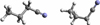 |
Fig. 1. Schematic depiction of the anti (left) and the gauche (right) conformers of n-PrCN. The C and N atoms are represented by gray and violet “spheres” respectively, and the H atoms by small, light gray ones. |
Belloche et al. (2009) identified a-n-PrCN (in its ground vibrational state) for the first time toward Sgr B2(N) a site of high-mass star formation, in a line survey using the IRAM 30 m telescope. Lines of the gauche conformer could be included correctly in their model but were too blended for a conclusive identification. Transitions of g-n-PrCN were later detected unambiguously along with the detection of i-PrCN. These identifications were made in a spectral line survey called Exploring Molecular Complexity with ALMA (EMoCA; Belloche et al. 2016). This survey, between 84.1 and 114.4 GHz was taken with ALMA toward Sgr B2(N). Müller et al. (2016), using the same survey, reported the identification of four vibrationally excited states for both anti- and gauche-n-PrCN following new spectroscopic work summarized in the last paragraph.
Laboratory measurements of n-PrCN in the vibrational ground states have been sufficient to detect this molecule in space for some time, however, it is only recently that predictions of some of the vibrational states have been good enough to envisage their detection. The ground state rotational constants of n-PrCN were first reported by Hirota (1962) following measurements up to 32 GHz. Demaison & Dreizler (1982) and Vormann & Dreizler (1988) used Fourier transform microwave spectroscopy to study the 14N quadrupole structure up to 26 GHz. The latter authors also studied the methyl internal rotation. Wlodarczak et al. (1988) extended the measurements up to 300 GHz and measured the dipole moment components. The energy difference between the two conformers is small leading to some confusion as to that of lower energy. The previous authors determined from intensity measurements that the anti conformer is lower in energy than the gauche by 1.1 ± 0.3 kJ mol−1. Durig et al. (2001) used infrared spectroscopy of n-PrCN dissolved in liquid Xenon to determine that the gauche conformer is lower than the anti by 0.48 ± 0.04 kJ mol−1 (or 58 ± 4 K) and Müller et al. (2016) found this value to be fully consistent with their model of the ALMA spectra.
Hirota (1962) also determined the rotational constants of the three lowest fundamental vibrational states of the anti and gauche conformers. The information of these excited states for both conformers is summarized in Table 1. Since no gas phase measurements are available the vibrational frequencies given are scaled abinito values from Durig et al. (2001). The nomenclature of the states differs from that in the aforementioned publication since although the gauche conformer has C1 symmetry, with all vibrations belong to the symmetry class a; the anti conformer has CS symmetry with 18 fundamental vibrations belonging to the symmetry class a′ and 12 to the symmetry class a″ (Crowder 1987). The equivalent energy for the a-n-PrCN includes the energy of this conformer above that of the gauche. As can be seen from the equivalent temperatures in Table 1, these vibrational states are predicted to be substantially populated in hot core regions of star-formation where temperatures can rise to around 100−300 K. For comparison the lowest vibrational states are around 525 K for methyl cyanide, 302 K for ethyl cyanide, as detailed above, and 266 K for i-PrCN. Recently, the laboratory spectroscopic study up to 127 GHz of these vibrationally excited states (Müller et al. 2016) led to their detection in space as explained above. Following this identification we decided to carry out a more extensive analysis up to 506 GHz of these vibrational states with the aim of providing reliable predictions over the whole operating band of ALMA. The present data should be useful to search for vibrationally excited states of n-PrCN in Orion KL where transitions of the ground vibrational states of both conformers were detected recently with ALMA (Pagani et al. 2017). During our work we also extended the spectral analysis of the ground state, and carried out new work on the combination states of v18 = v30 = 1 for the anti conformer and v29 = v30 = 1 for the gauche conformer. Transitions of these and other higher-lying vibrational states may be observable in the new EMoCA data obtained in ALMA Cycle 4.
Lowest fundamental vibrational states of n-PrCN.
2. Laboratory spectroscopic details
All measurements were carried out at Universität zu Köln. A schematic diagram of the experimental arrangement is shown in Fig. 2. The experimental arrangement for measurements between 36−70 GHz and between 89.25−126.75 GHz have been described previously (Müller et al. 2016). In the two new higher frequency ranges (171−251 and 310−506 GHz) we used a 5.1 m long double path (10.2 m total) absorption cell with inner diameter of 100 mm and equipped with Teflon windows. A commercial sample of n-PrCN was flowed slowly through the cell at pressures of around 1 Pa. The cell was at room temperature but the inlet system was heated to about 50°C to achieve a stable pressure in the cell and prevent condensation blocking the needle valve used for flow adjustment. Measurements between 171−251 GHz and between 310−506 GHz used a Virginia Diodes WR9.0 THz starter kit with cascaded multipliers and respectively 3 mW and 0.18 mW middle range output power. Toward the edges the power is around a factor of 15 smaller. This chain was driven by a Rohde & Schwarz SMF 100A synthesizer. From 171−251 GHz eighteen times multiplication and 63 kHz point spacing was used, from 310−506 GHz thirty six times and 144 kHz. We carried out large spectral scans of around 6−7 GHz taking typically several hours to acquire. Up and down scans were co-added. Schottky diode detectors were used to detect output power. We used frequency modulation (FM) throughout with demodulation at 2f, which causes an isolated line to appear approximately as a second derivative of a Gaussian. Optimally the FM deviation was set to half the linewidth, hence typically 250 kHz around 300 GHz. The sensitivity of the spectrometer systems varied with frequency showing both a diminution on the edges of the frequency bands and fluctuations throughout (source power, coupling, reflections, absorption by the optics) in spite of periodic optimization. Nevertheless, relative intensities could be used as guidance for assignments by comparing lines relatively close in frequency.
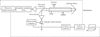 |
Fig. 2. Setup diagram for the molecular absorption spectra measurements. The arrow and dot between the wire-grid polarizer and tilted window express the polarizations of the incident and outgoing radiation. |
3. Spectroscopic results and discussion
3.1. Ground vibrational state
The frequency of previous fits of the ground states was limited to 300 GHz. Our latest fits of the vibrationally excited states were based on deviations from the ground-state parameters and were made up to 506 GHz. Hence we found it useful to also include new higher frequency measurements and make an up-dated fit of the ground state. The extension of the fit, and the increasing precision of predictions allowed us to also include 1002 additional transitions for the anti conformer and 1545 for the gauche in the range below 300 GHz, including b-type and hyperfine split transitions. The assigned uncertainties were 0.01−0.1 MHz, depending on the quality of lines. Usually uncertainties of 0.05−0.1 MHz were assigned above 310 GHz because of the very crowed spectrum which is caused for example by the increase of lines for a given J and the increase in line width (to more than 1 MHz). The difference in the components of the dipole moment for the anti and gauche conformers has an implication on the type of transitions that can be measured and on the parameters that can be determined as will be elaborated below. We took the following dipole moment components for our predictions: for a-n-PrCN, μa = 4.0 D, μb = 0.98 D, μc = 0 (by symmetry); for g-n-PrCN, μa = 3.27 D, μb = 2.14 D, μc = 0.45 D. Most of the values are those determined by Wlodarczak et al. (1988), however, μa for a-n-PrCN, and μc for g-n-PrCN were taken from quantum-chemical calculations made by H.S.P Müller using the method described in Müller et al. (2011). The value of μa for a-n-PrCN, some 10% larger than that quoted by Wlodarczak et al. (1988) is also consistent with astrophysical observations (Belloche et al. 2014).
In total we added 1992 new measured transitions (1284 lines because of transitions close or at the same frequency) for the anti conformer in the frequency bands of 36−70, 89−127, 171−251 and 310−506 GHz with Ka up to 29 and J up to 115 for the lower state (denoted K″a and J″). The fitted lines for the anti conformer are shown in Table 10 (available at the CDS, contains the following information: rotational transition represented by quantum numbers of upper and lower levels, assigned frequency, calculated frequency, residual (assigned−predicted), uncertainty assigned; and for non-resolved transitions: weighted average predicted frequency and difference from assigned frequency). In these newly assigned lines, there were 154 hyperfine split transitions and all of them could be fitted with the hyperfine structure parameters from Vormann & Dreizler (1988). The hyperfine split lines were all below 100 GHz, because of the increasing overlap and broadening of lines at higher frequencies. Besides mainly a-type transitions, 20 b-type lines were assigned and fitted. All transitions were R-branch because of their stronger intensities in a-n-PrCN. The assigned b-type R-branch lines with (ΔJ, ΔKa, ΔKc)=(1, ±1, 1) were in the frequency below 251 GHz and have a K″a up to 2 and J″ up to 55. Using the larger set of fitted lines, we were able to refine the molecular parameters which are listed in Table 2 together with the parameters determined in Belloche et al. (2009). By comparison we can see that uncertainties on the parameters are smaller. However, the WRMS of our fits is somewhat higher as it is close to or slightly less than 1, which indicates experimental uncertainties are comparable to residuals. We were also able to add some octic centrifugal distortion parameters (LKKJ, LJJK and LJ). We constrained the value of HK to the same value as its estimation in Belloche et al. (2009) since it could not be correctly fit because of the persistent lack of b-type transitions with higher values of Ka.
Molecular parameters for the ground vibrational states of n-PrCN obtained from our latest fit using Watson’s S reduction compared to the fit of Belloche et al. (2009).
We give some additional information to quantify the reliability of predictions. For R-branch a-type transitions the limit of good predictions is J″ = 123 at K″a = 32. This limit is specified for uncertainties on the predictions less than 0.1 MHz and a similar criterion will be used for the following sections. For lower Ka the limit in J increases slowly and for higher Ka it decreases rapidly as is the case for the examples that will be cited for the other conformer and other vibrational states.
For the gauche conformer, because of its more asymmetrical geometry and larger b-component of the dipole moment, more different types of transition (compared to the anti) were intense enough to be identified and assigned. Totally 3290 more transitions (1861 new lines) were fitted and shown in Table 11 (available at the CDS); they are 1318 R-branch a-type transitions, 143 Q-branch a-type transitions, 1255 R-branch b-type transitions, 448 Q-branch b-type transitions and 126 P-branch b-type transitions. All of the newly assigned Q- and P- branch lines are below 320 GHz. 442 hyperfine split transitions were included and fitted with parameters from Vormann & Dreizler (1988). Both a-n-PrCN and g-n-PrCN showed prolate pairing. Again due to the more asymmetrical geometry of g-n-PrCN only K″a = 0 and 1 lines could be found oblate paired for the anti conformer whereas for the gauche conformer oblate pairing could be observed up to between K″a = 7 and 8. The newly fitted lines of g-n-PrCN also allowed us to refine the parameter list as shown in Table 2, with all parameters showing uncertainties at least ten times lower than those quoted in Belloche et al. (2009). Additionally, higher order centrifugal distortion parameters: LJJK, LJ, l1 and PKKKJ could be determined. As regards good predictions (see the anti conformer) the limit of R-branch a-type transitions is for example J″ = 99 at K″a = 50. Considering oblate pairing at high frequencies, transitions with (ΔJ, ΔKa, ΔKc)=(1, 1, 1) were used to make confident predictions. Finally, all b-type transitions at frequencies below 950 GHz were well predicted with K″a up to 34.
3.2. v30 = 1 and 2 of g-n-PrCN
v30 = 1 is the lowest-lying vibrationally excited state of g-n-PrCN which corresponds to a C2H5 torsion around the central C atom (Crowder 1987; Müller et al. 2016). In this work, measurements at 171−251 and 310−506 GHz were added to refine the parameters; the frequency of transitions was limited to 127 GHz in Müller et al. (2016). We assigned new lines in the sequence of increasing J for each Ka first in the lower frequency range and then for the higher one, so as to carefully check the coherence of the evolution of molecular parameters. When new lines could not be fit within experimental uncertainties, and especially when trends were observed, new additional parameters were tried sequentially. The final derived parameters with their uncertainties are listed in Table 3 and those determined in Müller et al. (2016) are listed simultaneously as comparison. Lines of v30 = 1 and v30 = 2 were fit together. We followed the method for coding the parameters of vibrationally excited states used in previous papers, that is ΔX represents Xv = 1 − Xv = 0, and ΔΔX = Xv = 2 − Xv = 0 − 2ΔX. Using this method, we took advantage of the relation between vibrational states to reduce the number of parameters needed to be determined. Furthermore, ΔX should be significantly smaller than Xv = 0, and ΔΔX significantly smaller than ΔX, giving a useful check on parameters with abnormal values. The decrease in intensities of lines of higher excited states made their fitting more difficult, especially at high frequency. Finally we could fit 2632 more transitions (1524 new lines) for v30 = 1. All of the newly fitted 1457 a-type transitions were R-branch with ΔKa = 0; we tried to find Q-branch a-type lines but they were much weaker (for example for two lines compared around 178.9 GHz the Q-branch a-type transition was about 50 times weaker than a nearby R-branch a-type transition). The highest J″ of a-type lines we could fit in our available frequency was around 90 near 500 GHz, with somewhat higher values for low Ka and somewhat lower values for high Ka. We fitted a-type transitions with K″a up to 20 over all ranges, and an additional 32 transitions with K″a between 21 and 25 between 171−251 GHz. Like in the ground state, a-type high J low Ka transitions were usually oblate paired with b-type transitions in the same branch. Totally 1175 b-type transitions in both R- and Q-branches were added to the fit. Most b-type transitions assigned were R-branch and more occurred in the high frequency range as the energy between neighboring Ka levels gets larger quickly with increasing Ka. Among the newly fitted R-branch b-type transitions about half had (ΔJ, ΔKa, ΔKc)=(1, 1, 1) with K″a covering 0 to 19, while the transitions with (1, −1, 1) all had K″a up to 12 and the transitions with (1, 1, −1) had K″a not less than 6. Among the Q-branch, previously fitted transitions have K″a less than 12 between 37.30−125.54 GHz, and 204 newly fitted transitions were all b-type with K″a ≤ 12 between 171−251 GHz. The refined parameters enable good predictions (see Sect. 3.1) of R-branch a-type transitions up to J″ = 91 at K″a = 30, and b-type transitions with (ΔJ, ΔKa, ΔKc)=(1, 1, 1) up to J″ = 95 at K″a = 20.
Changes of molecular parameters for the v30 = 1 and 2 vibrational states of g-n-PrCN obtained from our latest fit using Watson’s S reduction compared to the fit of Müller et al. (2016).
Fitted transitions of v30 = 2 above 171 GHz were similar in type to those of v30 = 1: 1045 R-branch a-type transitions, 778 R-branch b-type transitions, and 214 Q-branch b-type transitions; with no new hyperfine split transitions. Table 12 (available at the CDS) gives all lines of v30 = 1 and v30 = 2 used in the final fit. We found it was difficult to fit a-type transitions with J″ larger than 89 for K″a = 0 and 1, as all these transitions showed residuals (assigned−predicted) with a trend of increasing negative values. New parameters could not be determined to remove this trend. Therefore we put all these identified transitions in a separate list (Table 13, at the CDS). As a precaution, all same-type transitions with J″ larger than 89 for higher K″a were put into this supplementary list even if the lines appeared to fit correctly. An obvious trend of residuals also took place with J″ larger than 59 for K″a = 20. The limit of safe a-type lines climbs to K″a = 22 with J″ up to 58. R-branch b-type transitions in our newly assigned frequency ranges could be classified in 3 groups as was the case for v30 = 1: transitions with (ΔJ, ΔKa, ΔKc)=(1, 1, 1),(1, −1, 1) and (1, 1, −1). All 3 groups of transitions are in the frequency ranges of 171−251 and 310−506 GHz, with the coverage of Ka and J similar to those of v30 = 1. The Q-branch b-type transitions with (ΔJ, ΔKa, ΔKc)=(0, 1, −1) are all in the range 171−251 GHz with K″a from 12−17, J″ from 19−65 and not sequential with frequency. The two sub-branches of the Q-branch b-type transitions (J = Ka + Kc and J = Ka + Kc − 1) show prolate pairing and hence have doubled intensities facilitating the assignments. Taking into account that vibrational coupling may cause some transitions to shift in frequency by up to the order of 1 MHz, safe predictions can be made up to J″ = 88 at K″a ≤ 19 and J″ = 59 for 20 ≤ K″a ≤ 25 for a-type transitions, and up to K″a = 14 for b-type transitions.
3.3. v29 = 1 of g-n-PrCN
v29 = 1 is a vibrational state lying in energy between v30 = 1 and v30 = 2. We started from the fit of Müller et al. (2016) and first added lines up to 251 GHz. When we got to K″a = 8 for new lines we started to have problems with a calculated WRMS larger than 1.40. We noticed that Q-branch b-type lines with high J numbers in Müller et al. (2016) all had residuals more than three times the attributed uncertainties (3σ) with the same sign for a particular K″a. We decided to remove these problem lines from the fit, and concentrate on Q-branch b-type transitions at higher frequency which have stronger intensities (176 transitions with K″a between 12−17 at 176−242 GHz). The newly determined parameters allowed us to make more precise predictions and identify clearly that the problem lines show internal rotation splitting, that was previously difficult to differentiate from line crowding and quadrupole hyperfine splitting. The split lines show two components separated by around 0.5 MHz with similar intensity and center on the up-dated predictions. The center frequencies (all calculated by averaging the positions of the two components) were hence assigned with a higher uncertainty (0.05 MHz). All lines included in our new fit up to 506 GHz are listed in Table 14 (at the CDS). No hyperfine splitting was resolved above 171 GHz, while all lower-frequency hyperfine split lines from Müller et al. (2016) were fitted with the ground-state hyperfine structure parameters from Vormann & Dreizler (1988). If not indicated specifically, it is the same for other states. R-branch b-type transitions were in the same three groups as v30 = 1 and 2, with the largest K″a = 19 and largest J″ = 91 near 500 GHz. The b-type transitions with (ΔJ, ΔKa, ΔKc)=(1, 1, ±1) are prolate paired (or close) with low J″ and high K″a; while (1, ±1, 1) transitions are more oblate paired with high J″ and low K″a, therefore nearly half of the newly assigned, 715 R-branch b-type transitions had (ΔJ, ΔKa, ΔKc)=(1, 1, 1). All newly assigned R-branch a-type transitions with K″a up to 20 and 32 were successfully fit at frequencies up to respectively 506 and 251 GHz. a-type transitions with K″a = 11 were badly fit above J″ = 77 for the sub-branch J = Ka + Kc and J″ = 82 for J = Ka + Kc − 1 with obvious trends. We put all these lines, with lines of larger J″ and K″a (even if some had reasonable residuals), into a separate list (Table 15, available at the CDS) as we did in v30 = 2 and they were excluded from our final fit. Finally we derived the parameter list as shown in Table 4 additionally determining ΔHK and Δh1. ΔHJK was decreased by 60% compared with Müller et al. (2016), because of the correction of the assignment of lines with internal rotation splitting. These corrected transition frequencies as well as the newly assigned transitions allowed us to determine Δh1 and this, in turn, changed the values of Δh2 and Δh3 significantly. The value of ΔHJ was also better determined. The refined parameters allow confident predictions above 310 GHz for a-type transitions with J″ up to 121 at K″a = 10, but less than 77 at K″a between 11 and 35. For b-type transitions, the largest K″a is 14.
Changes of molecular parameters for the v29 = 1 vibrational states of g-n-PrCN obtained from our latest fit using Watson’s S reduction compared to the fit of Müller et al. (2016).
3.4. v28 = 1 of g-n-PrCN
Most transitions fitted in Müller et al. (2016) were R-branch a-type with J″ less than 22 and K″a less than 19. The v28 vibrational mode involves mainly methyl group torsion (Crowder 1987; Durig et al. 2001) leading to a considerable internal rotation character in the microwave spectra; some evidence was observed in Müller et al. (2016) when assigning transitions with K″a ≥ 3. Owing to this, our confident assignments for the high-KR-branch a-type transitions could not climb as high in J″ as the lower-energy states of g-n-PrCN: J″ = 40 between K″a = 10 − 20 at about 245 GHz. Since the internal rotation causes broadening, shoulders or splits which are more prominent in high J transitions, we followed a similar procedure to Müller et al. (2016). For symmetric broadening, or splits with similar intensities of the two components with the separation around 0.6 MHz, we assigned the prediction to the center and gave an uncertainty of 0.05 MHz. For splits with an intensity ratio of 1:2 or 2:1, we assigned the prediction to the weighted average frequency and gave an uncertainty of 0.10 MHz. This is indicated in the line lists available at the CDS. The broadening and line density above 310 GHz made secure assignments for internal-rotation affected lines impossible; finally a-type transitions could be fit with K″a up to 9 between 310−506 GHz. The small number of b-type transitions fitted in Müller et al. (2016) made it difficult to determine the pure K parameters, DK and HK. For R-branch b-type transitions, the assignments with higher K″a were difficult because they were close to each other. This was already the case at lower frequency as described in Müller et al. (2016). However, 309 R-branch b-type transitions with (ΔJ, ΔKa, ΔKc)=(1, ±1, 1) whose K″a up to 9 and J″ up to 89 could be added to the fit up to 506 GHz. Because of the difficulty in assigning high-K transitions, it was not possible to add new (1, 1, −1) transitions at higher frequency. Additionally, 12 new Q-branch b-type transitions could be assigned and fit; all of these lines have K″a between 12−17 from 174.93−245.03 GHz. These newly assigned b-type transitions proved useful to determine the molecular parameters especially ΔDK, whose value was freed and determined consistent to the estimation in Müller et al. (2016; as Table 5). All fitted lines of v28 = 1 can be found in Table 16 (available at the CDS) and additional lines were put in Table 17 (available at the CDS) as we did for other states of the gauche conformer. The limit of good predictions above 310 GHz is J″ = 89 at K″a up to 5 and J″ = 78 at larger K″a (≤9) for both a- and b-type transitions, owing to the difficulty in assigning high-K transitions.
Changes of molecular parameters for the v28 = 1 vibrational states of g-n-PrCN obtained from our latest fit using Watson’s S reduction compared to the fit of Müller et al. (2016).
3.5. v29 = v30 = 1 of g-n-PrCN
Hirota (1962) refers to seeing combination states in his measurements but gives no further details or analysis. We used the empirical method of estimating the parameters by addition of the changes of each individual vibrational state: Xv29 = v30 = 1 = Xv = 0 + ΔXv30 = 1 + ΔXv29 = 1 + ΔΔX. First predictions were made with ΔΔX = 0. Lines could then be easily assigned to transitions with low quantum numbers, and subsequently the correction ΔΔX was liberated for certain parameters to fit successively more transitions. The exploratory assignments began with intense R-branch a-type transitions and then b-type transitions. After all R-branch transitions were assigned and fitted, Q-branch b-type transitions were measured with particular care because of the already identified internal rotation of v29 = 1 involved in the movement of this combination vibrational state and the higher energy giving weaker lines. For R-branch a-type transitions, we could successfully fit all transtions with K″a up to 20 (excluding lines of K″a = 18, which showed a clear trend in residuals between 197.48 and 221.45 GHz) for frequencies below 251 GHz. But in the range 310–506 GHz, the assignments appeared difficult in spite of larger intensities. As for other vibrational states of g-n-PrCN, the oblate pairing consisting of a-type and b-type transitions facilitated the assignments. However, the increasing separation of paired transitions with increase in quantum numbers made assignments more difficult combined with the blending and broadening in the high frequency range and the possible splits caused by internal rotations. Therefore very secure assignments with K″a up to 4 or 5 (for each sub-branch) were first made. Even after the improvement of the parameters several lines at each K″a could not be correctly fitted showing systematic residuals. All these lines are in the ranges of J″ from 68 to 73 and from 89 to 93. We attributed this as due coupling with other vibrational states. Finally 935 R-branch a-type transitions were identified in all four frequency ranges. The assignment of b-type transitions was not easy due to low intensities at low frequencies and blending and broadening at high frequencies. The confidently assigned b-type transitions at high frequency were all oblate paired with intense a-type transitions with K″a less than 6. Totally, 487 b-type transitions were fitted. Q-branch b-type transitions were useful to correctly determine the parameter DK. We identified internal rotation causing splits (with the components separated by around 0.6 MHz) at frequencies between 89.25–126.75 GHz, in transitions with large J″. In this range, Q-branch b-type transitions have K″a less than 11 and those that could be securely assigned have J″ less than 45. For Q-branch b-type transitions with K″a between 13 and 18 in the range 171–251 GHz, only prolate pairs were assigned. These transitions have low J″ and hence are not affected by internal rotation. Finally 466 Q-branch b-type transitions were correctly fitted. Moreover, 110 hyperfine split transitions were fitted with fixed hyperfine parameters from v30 = 1. These are R-branch a-type transitions with J″ approaching K″a (less than 11), b-type transitions (both R-branch and Q-branch) with K″a less than 4 at frequencies below 70 GHz. The derived parameters are shown in Table 6. The fitted transitions are in Table 18 (available at the CDS), and those confidently assigned but not correctly fitted with systematic residuals are separated in Table 19 (available at the CDS). Using the newly derived molecular parameters, confident predictions of a-type transitions can be made up to J″ = 68 for K″a ≤ 5 below 380 GHz, and J″ = 41 for K″a ≤ 41 below 251 GHz (excluding lines of K″a = 18 that show residuals that cannot be fitted). For b-type transitions, all R-branch predictions with K″a ≤ 11 below 251 GHz are reliable, and J″ ≤ 41 for K″a ≤ 17 for the Q-branch also below 251 GHz. For frequencies above 310 GHz, the limit of b-type transitions has the same limit as the a-type because of oblate pairing.
Changes of molecular parameters for the v29 = v30 = 1 vibrational states of g-n-PrCN obtained from our latest fit using Watson’s S reduction.
3.6. v30 = 1 of a-n-PrCN
v30 = 1 of a-n-PrCN was fit together with v30 = 2 and v18 = 1, in order to take into account Coriolis-type and Fermi coupling effects between the latter two states. All lines of v30 = 1, 2 and v18 = 1 included in the final fit are given in Table 20 (available at the CDS). All confident assignments showing large residuals and a trend that could not be corrected with additional parameters were put in a separate list (Table 21, available at the CDS) as was done for the gauche conformer. Finally we obtained changes of the molecular parameters for all three vibrational states shown in Table 7. We discuss v30 = 1 first. Most transitions fitted were a-type (516 out of 540 in Müller et al. (2016); 1134 new transitions out of 1259 in this work) because of the low value of μb. New assignments between 171−251 GHz could be smoothly fit for all a-type transitions with K″a up to 19, by adding ΔHJK. For K″a = 20, transitions with J″ between 38−48 between 173−217 GHz could not be correctly assigned because of the poor line shape; assignments could be made with larger J″, but the residuals were already over our acceptable value (3σ). For assignments between 310−506 GHz, we were only able to fit up to K″a = 3 with the previous parameter list. First we tried to add Δh1 and Δh2, as h1 and h2 could be determined for the ground vibrational state but these parameters did not allow us to fit higher K″a lines correctly. In order to do this we had to add Δh3, but in this case Δh1 could not be determined any more. Finally the best fit was obtained using Δh2 and Δh3. For lines above 310 GHz, we could not successfully fit above J″ larger than 84 for K″a = 14 with all problem lines showing negatively trended residuals. Similarly K″a = 15 showed positive trended residuals and 16 positive trended but smaller residuals. The addition of high order parameters did not allow an adequate fit of these lines, and the value of parameters varied largely and became dependent on the data set used. We hence omitted them from the final fit. Although K″a = 17, 18 and 19 could then be fitted with all determined parameters, by precaution we put all lines with J″ > 84 and K″a > 13 into our separate list in Table 21. Extensive fitting of b-type lines proved difficult. We did, however succeed in measuring 125 b-type transitions, up to 251 GHz. Most of these b-type transitions are Q-branch with K″a up to 3 because of their higher intensities. For R-branch b-type transitions we could get to J″ = 55 and K″a = 2. b-type lines were very useful for determining ΔA and ΔDK, whose uncertainties were decreased to one tenth of their previous values (as Table 7). The value of HK in the ground-state of a-n-PrCN could not be correctly determined, and no differences (ΔHK) were hence determined for the vibrationally excited states. Using the new parameters, predictions should be relatively confident with J″ up to 119 for K″a ≤ 28, but predictions for K″a = 14, 15 and 16 with J″ ≥ 84 may not all be reliably precise because of the vibrational coupling. Hence the measured frequency should be used when available.
Changes of molecular parameters for the v30 = 1, 2 and v18 = 1 vibrational states of a-n-PrCN obtained from our latest fit using Watson’s S reduction compared to the fit of Müller et al. (2016).
3.7. v30 = 2 and v18 = 1 of a-n-PrCN
The fitting for v30 = 2 was started after the parameters of v30 = 1 were obtained. We first fitted the transitions from 171−251 GHz with increasing K″a. For K″a = 9, transitions with J″ between 43−55 could not be correctly fit, neither could the transitions with K″a = 10 and 11. Our new assignments with higher values of K″a in the final line list enabled us to determine ΔΔHKJ which took a larger than estimated value of about three times ΔHKJ. This then allowed lines with K″a up to 11 to be successfully fit. We then started to assign lines of v18 = 1 at 171−251 GHz, since no major coupling had been observed previously up to this K″a value. Lines with K″a up to 12 could be fit for v18 = 1. However, lines with higher K″a were calculated with residuals beyond our expectance. After including the new data, previously assigned v30 = 2 lines with K″a = 12 and 13 had positive residuals above 3σ whereas residuals with negative values could be found for previous assignments of v18 = 1 with K″a = 13 and 14. For K″a = 14 of v30 = 2, residuals were between −0.22 to −0.30 MHz for previous assignments. These deviations are likely caused by deficiencies in describing the Coriolis-type interaction between v18 = 1 and v30 = 2. In contrast, the residuals for K″a = 15 of v18 = 1 were positive with almost same absolute values as v30 = 2. Restraining ΔΔHKJ as Müller et al. (2016), did not help. We attributed the problem to insufficient coupling parameters, and determined that GcJ and FK were necessary for fitting these lines. The effect of adding these two parameters is shown in Fig. 3. We could then fit lines of v30 = 2 with K″a up to 19. Lines with K″a = 19 above J″ = 51 showed asymmetrical shapes and even splits. For v18 = 1 we could safely assign and fit lines with K″a up to 20. We then moved on to the higher frequency range above 310 GHz. Fitting was successful for K″a = 8 for v30 = 2 up to 506 GHz, but at K″a = 9 we were hindered by separation of transitions from their prolate pairs at J″ = 95, which lead to a broadening of the line shape or even unresolved splits. Fitting with higher K″a proved difficult, and at higher energy, coupling with other vibrational states is possible. We noticed obvious trends in the residuals of lines with K″a ≥ 10. For example, positive-trend residuals (0.12 to 0.31 MHz) for J″ between 83−111 at K″a = 10, negative-trend residuals (−0.08 to −1.46 MHz) for J″ between 84−109 at K″a = 11. Lines showing identified trends in the residuals with K″a up to 17 are listed in Table 21; higher K″a lines could not be followed and assigned confidently. For v18 = 1, the separation of sub-branches of R-branch a-type transitions also stopped us fitting transitions with J″ larger than 85 at K″a = 9. Up to K″a = 16, assignments could be correctly fit up to J″ = 76 at around 336 GHz; the fits for higher J″ transitions with trended residuals are included in Table 21. We could successfully fit another 25 b-type transitions with K″a = 0 and 1 for v30 = 2 that are included in Table 20 (available at the CDS), most of them R-branch transitions between 171−251 GHz. For these two states, confident predictions should be possible up to J″ = 110 for K″a ≤ 9; for higher K″a ≤ 17 confident predictions are limited to J″ ≤ 82. Note that interstate transitions between v30 = 2 and v18 = 1 can be predicted but are too weak to be measured in laboratory and most certainly in space.
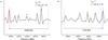 |
Fig. 3. Spectral extracts showing the effect of coupling parameters. The dot dash lines are predictions without coupling parameters; the dashed lines show predictions with coupling parameters from Müller et al. (2016) and the solid lines show predictions with additional coupling parameters determined in this work. Lines for other identified transitions are shown in the figures as well: • for ground state of a-n-PrCN, for v30 = 1 of a-n-PrCN, ° for v30 = 1 of g-n-PrCN, and × for v29 = 1 of g-n-PrCN. |
The difficulty of the fits for v30 = 1, 2 and v18 = 1 of a-n-PrCN is increased by a non-resonant Coriolis interaction between v30 = 1 and v18 = 1. This interaction is apparent in the relatively large vibrational corrections of many spectroscopic parameters of v18 = 1 and v30 = 2 which are often of similar magnitude, but of opposite sign (see Table 7). Fitting of the entire present data set may thus require more changes in spectroscopic parameters than can safely be determined. Because of the multiple interactions possible between several vibrational states the determination of these parameters most likely requires substantial further measurements and analysis that are outside the scope of this work for predicting lines strong enough to be clearly seen in an astrophysical survey. However, this may be done in future.
3.8. v29 = 1 of a-n-PrCN
v29 = 1 of the anti conformer is a vibrational state with energy between v30 = 2 and v18 = v30 = 1. The assignments for transitions in higher states were difficult since their intensities get weaker and because the possibility of coupling with other states increases. As explained previously the identification of b-type transitions was even harder. Since only a-type transitions with ΔKa = 0 were identified it was not possible to determine ΔDK. ΔA was not so well determined. We could identify internal rotation splitting caused by the methyl group torsion with K″a = 1 and 2 (only for the sub-branch, J = Ka + Kc). All of the split lines showing similar-intensity components separated by around 0.5 MHz, are between 171−251 GHz, with J″ between 39−57 (for K″a = 1) and between 46−55 (for K″a = 2). At higher frequencies internal rotation splitting and accidental line overlap could not be discriminated and hence assignments were not made if a single symmetric line was not identified. Finally, transitions with K″a up to 17 could be fit between 171−251 GHz with J″ between 39 and 58. Above 171 GHz transitions with K″a = 11 could not be correctly fit, with residuals from 0.43 to 1.53 MHz showing a trend with increasing J″. This is probably due to coupling with another vibrational state, as other K″a transitions (above and below) in the frequency range could be well fitted. For assignments from 310−506 GHz, we could fit transitions with K″a up to 8. For weaker none-prolate paired transitions with K″a less than 8, overlaps stopped us fitting more transitions, especially those with K″a from 4 to 7. Higher K″a transitions were assigned but all with trends in the residuals, and were removed to the supplementary list given in Table 23 (available at the CDS) with all assigned K″a = 11 transitions not included in the fit. Explorative fits including transitions with K″a = 9 and 10 at 310−506 GHz changed determined parameters significantly and required illogical higher order parameters. Also the fits became dataset dependent since the newly determined parameters fit transitions with even higher K″a, worse than the previous. Therefore all assignments of transitions with K″a ≥ 9 were moved to Table 23 leaving transitions included in the fit in Table 22 (available at the CDS). Finally the changes of parameters are shown in Table 8. Confident predictions can be made with K″a ≤ 8 with good results (see section 3.1) for J″ up to 90. Higher K″a predictions can be made with relative confidence especially at lower frequencies except for K″a = 11 because of the unidentified vibrational coupling.
Changes of molecular parameters for the v29 = 1 vibrational states of a-n-PrCN obtained from our latest fit using Watson’s S reduction compared to the fit of Müller et al. (2016).
3.9. v18 = v30 = 1 of a-n-PrCN
We present in Table 9 the first published molecular parameters for v18 = v30 = 1 of a-n-PrCN. Hirota (1962) refers to seeing combination states in his measurements but gives no further details or analysis. The assignments were quite difficult as this state has the highest energy in our present study. Moreover, just as v18 = 1 and v30 = 2 interact resonantly, v18 = v30 = 1 and v30 = 3 are expected to interact resonantly, and v18 = v30 = 1 is expected to interact at least non-resonantly with v30 = 2 and with v18 = 2. Finally 613 transitions (492 lines) were assigned and fitted below 506 GHz (Table 24, available at the CDS). All transitions assigned are a-type R-branch because of their strong intensities. At the beginning, only parameters of v30 = 1 and v18 = 1 were used to make predictions, that can be seen from the table to give relatively correct estimates of B, C and DJ. These estimates were sufficiently correct, along with the other approximate parameters, to identify lines with K″a between 0 and 5 below 70 GHz. Then more lines could be identified with iterative fitting and refinement of the parameters. Lines were assigned sequentially through all four available frequency ranges: 36−70, 89−126, 171−251, and 310−506 GHz as increasing J″ and K″a. We could safely assign transitions with the highest K″a = 8 in all available frequency ranges. Below 70 GHz we were able to assign some additional lines (J″ between 10 and 14 for K″a = 9; J″ between 11 and 13 for K″a = 10). Assignments for higher K″a transitions need high order centrifugal distortion parameters, which are also better determined by fitted transitions with high quantum numbers. Lower intensities of higher K″a transitions and possible coupling with v29 = 1 presented ambiguities for their assignments. Conversely lack of lines with high K″a make it difficult to characterize any coupling with v29 = 1. Exploratory fits for transitions with K″a = 9 and 10 between 89−126 GHz resulted in negative residuals of about −0.2 MHz (20 ≤ J″ ≤ 22) and −0.36 – −0.45 MHz (20 ≤ J″ ≤ 24) respectively, however without any clear trends; all these tentative assignments are listed in Table 25 (available at the CDS). Other assignments fitted with significant residuals (showing that more parameters are needed), include lines with 51 ≤ J″ ≤ 55 of K″a = 8 at 230.61−248.34 GHz (residuals between 0.09−0.34 MHz) and 90 ≤ J″ ≤ 111 of K″a = 1 at 396.84−486.70 GHz (residuals between −0.16 – −0.36 MHz). The WRMS we derived was somewhat larger than other states because high frequency lines were somewhat less well predicted with the current parameter list. We note that including ΔΔHKJ in the fit gave a determined value of −547(43)×10−9, however, since this value was unreasonably large we did not use it in the final fit. When J approaches Ka, broadening and splitting caused by quadrupole hyperfine splitting were identified. 58 hyperfine split transitions below 70 GHz were added to the list with K″a between four and ten. Hyperfine structure parameters from Vormann & Dreizler (1988) for the ground state are sufficient to fit them. Confident predictions are possible up to K″a = 7, for J″ ≤ 89. For K″a = 8, up to J″ = 50 and for K″a = 9 and 10, only predictions below 70 GHz can be treated with full confidence.
Changes of molecular parameters for the v18 = v30 = 1 vibrational states of a-n-PrCN obtained from our latest fit using Watson’s S reduction.
4. Conclusion and outlook
We have added 11453 new lines to fits for both conformers of n-PrCN, mainly in the frequency ranges 171−251 and 310−506 GHz. We have hence improved molecular parameters for the ground states of both anti- and gauche-n-propyl cyanide and for excited vibrational states of the gauche conformer (v30 = 1, v29 = 1, v30 = 2, v28 = 1) and anti conformer (v30 = 1, v18 = 1, v30 = 2, v29 = 1). The inclusion of these newly assigned lines gives a more precise and extended list of molecular parameters to improve the predictions over the entire operating range of ALMA. The present data should be useful to search for vibrationally excited states of n-PrCN in Orion KL with ALMA. For Coriolis and Fermi coupling between v30 = 2 (K″a ≥ 13) and v18 = 1 (K″a ≥ 14), two more coupling parameters FK and GCJ were derived from fitting. During the analysis, we not only continued assigning internal rotation split transitions in v28 = 1 of g-n-PrCN between 171−251 GHz but also identified additional internal rotation splitting of the Q-branch b-type transitions occuring in v29 = 1 (for both the fundamental and combination states) of the gauche conformer at frequencies below 125 GHz and also in the R-branch a-type transitions in v29 = 1 of the anti conformer with K″a = 1 and 2, at 171−251 GHz. This splitting is not expected to be resolved in astrophysical spectra. We gave the first published measurements and derived parameters for the combination state v18 = v30 = 1 for a-n-PrCN and for the combination state v29 = v30 = 1 for g-n-PrCN, both found by using our parameters for the individual vibrational states. Transitions of these and other higher lying vibrational states may be observable in the new EMoCA data obtained in ALMA Cycle 4. After each state and conformer, the reliability of predictions is discussed in particular as regards vibrational coupling, and limits of quantum numbers and frequencies are given. No problems have been found with the ground states. For the vibrational states above the limits given, it is best to use the measured frequencies given in the CDS when available. Measurements are presently not available in the ranges: 70−89, 127−171, and 251−310 GHz. As most of the perturbations observed are above about 350 GHz, confident predictions are available in these gaps. However, there are some particular cases. For v29 = 1 of the anti conformer, lines of K″a = 11 are perturbed above 176 GHz hence no confident frequencies are available in the highest frequency gap. Similarly for the combination state v29 = v30 = 1 of the gauche conformer, for K″a = 18 there are no confident frequencies available in the highest frequency gap. For the combination state v18 = v30 = 1 of the anti conformer, confident data is not available if not measured above K″a = 8 for frequencies above 70 GHz, and for K″a = 8 for frequencies above 221 GHz.
Lines assigned but not fitted correctly with our up-dated parameters are given as separate lists for astrophysical identification and will require future work to identify other vibrational couplings. These lines either have a shift more than three times the estimated experimental uncertainty or show clear trends in deviation, or both. Also lines that fit correctly but above Ka and J ranges already showing deviations have been included in the supplementary list and not in the fit by precaution. There is most likely in a-n-PrCN, a non-resonant interaction between v30 = 1 and v18 = 1 as indicated by large but opposite variations in the determined ΔA rotational constant. v30 = 2 is also probably affected by coupling with nearby states. Hence full treatment of the perturbed lines most likely requires the measurement at higher sensitivity of several additional higher vibrational states such as v30 = 3 and v18 = 2 by combined analysis. Tentative attempts to identify transitions of v30 = 3 in both conformers by extrapolation of the parameters from v30 = 0, 1 and v30 = 2 have not as yet been successful and require further work. Measurements of gas-phase rovibrational spectra in the far infrared may also provide useful data for a more extensive analysis. Evidence for coupling in the gauche conformer is also seen but affects less the fitting. In general fitting of the gauche conformer is easier because the higher asymmetry allows more parameters to be determined independently.
Acknowledgments
The work in Cologne was supported by the Deutsche Forschungsgemeinschaft (DFG) through the collaborative research grant SFB 956 project B3 and through the Gerätezentrum “Cologne Center for Terahertz Spectroscopy”. D.L. and A.W. thank PCMI for funding visits to Cologne for measurements and discussion with collaborators. PCMI is the French program “Physique et Chimie du Milieu Interstellaire” funded by the Conseil National de la Recherche Scientifique (CNRS) and Centre National d’Etudes Spatiales (CNES). They also thank the DFG via SFB 956 project B3 for funding additional-visits to Cologne. D.L. thanks the Chinese Scholarship Council (CSC) for funding his PhD study in France.
References
- Avery, L., Bell, M., Cunningham, C., et al. 1994, ApJ, 426, 737 [NASA ADS] [CrossRef] [Google Scholar]
- Belloche, A., Garrod, R., Müller, H., et al. 2009, A&A, 499, 215 [NASA ADS] [CrossRef] [EDP Sciences] [Google Scholar]
- Belloche, A., Müller, H. S., Menten, K. M., Schilke, P., & Comito, C. 2013, A&A, 559, A47 [NASA ADS] [CrossRef] [EDP Sciences] [Google Scholar]
- Belloche, A., Garrod, R. T., Müller, H. S., & Menten, K. M. 2014, Science, 345, 1584 [NASA ADS] [CrossRef] [PubMed] [Google Scholar]
- Belloche, A., Müller, H., Garrod, R., & Menten, K. 2016, A&A, 587, A91 [NASA ADS] [CrossRef] [EDP Sciences] [Google Scholar]
- Cernicharo, J., Agúndez, M., Kahane, C., et al. 2011, A&A, 529, L3 [NASA ADS] [CrossRef] [EDP Sciences] [Google Scholar]
- Clark, F., Brown, R., Godfrey, P., Storey, J., & Johnson, D. 1976, ApJ, 210, L139 [NASA ADS] [CrossRef] [Google Scholar]
- Crowder, G. 1987, J. Mol. Struct., 158, 229 [NASA ADS] [CrossRef] [Google Scholar]
- Daly, A. M., Bermúdez, C., López, A., et al. 2013, ApJ, 768, 81 [NASA ADS] [CrossRef] [Google Scholar]
- Demaison, J., & Dreizler, H. 1982, Z. Naturforsch. A, 37, 199 [NASA ADS] [CrossRef] [Google Scholar]
- Demyk, K., Wlodarczak, G., & Carvajal, M. 2008, A&A, 489, 589 [NASA ADS] [CrossRef] [EDP Sciences] [Google Scholar]
- Durig, J., & Li, Y. 1974, J. Mol. Struct., 21, 289 [NASA ADS] [CrossRef] [Google Scholar]
- Durig, J. R., Drew, B. R., Koomer, A., & Bell, S. 2001, Phys. Chem. Chem. Phys., 3, 766 [CrossRef] [Google Scholar]
- Fortman, S. M., McMillan, J. P., Neese, C. F., et al. 2012, J. Mol. Spectrosc., 280, 11 [NASA ADS] [CrossRef] [Google Scholar]
- Friedel, D. N., Snyder, L., Remijan, A. J., & Turner, B. 2005, Astrophys. J. Lett., 632, L95 [NASA ADS] [CrossRef] [Google Scholar]
- Gibb, E., Nummelin, A., Irvine, W. M., Whittet, D., & Bergman, P. 2000, ApJ, 545, 309 [NASA ADS] [CrossRef] [PubMed] [Google Scholar]
- Goldsmith, P., Krotkov, R., Snell, R., Brown, R., & Godfrey, P. 1983, ApJ, 274, 184 [NASA ADS] [CrossRef] [Google Scholar]
- Groesbeck, T., Phillips, T., & Blake, G. A. 1994, Astrophys. J. Suppl. Ser., 94, 147 [NASA ADS] [CrossRef] [Google Scholar]
- Guélin, M., Cernicharo, J., Navarro, S., et al. 1987, A&A, 182, L37 [NASA ADS] [Google Scholar]
- Guilloteau, S., Omont, A., & Lucas, R. 1987, A&A, 176, L24 [NASA ADS] [Google Scholar]
- Herberich, G. E. 1967, Z. Naturforsch. A, 22, 543 [NASA ADS] [Google Scholar]
- Hirota, E. 1962, J. Chem. Phys., 37, 2918 [NASA ADS] [CrossRef] [Google Scholar]
- Hollis, J., Lovas, F., Suenram, R., Jewell, P., & Snyder, L. 1983, ApJ, 264, 543 [NASA ADS] [CrossRef] [Google Scholar]
- Kobayashi, K., Ogata, K., Tsunekawa, S., & Takano, S. 2007, Astrophys. J. Lett., 657, L17 [NASA ADS] [CrossRef] [Google Scholar]
- Kolesniková, L., Alonso, E., Mata, S., Cernicharo, J., & Alonso, J. 2017, Astrophys. J. Suppl. Ser., 233, 24 [Google Scholar]
- Lovas, F., Suenram, R., Snyder, L., Hollis, J., & Lees, R. 1982, ApJ, 253,\pg{\break} 149 [NASA ADS] [CrossRef] [Google Scholar]
- Lucas, R., & Cernicharo, J. 1989, A&A, 218, L20 [NASA ADS] [Google Scholar]
- Mauersberger, R., Henkel, C., & Wilson, T. 1988, A&A, 205, 235 [NASA ADS] [Google Scholar]
- Mehringer, D. M., Pearson, J. C., Keene, J., & Phillips, T. G. 2004, ApJ, 608, 306 [NASA ADS] [CrossRef] [Google Scholar]
- Motiyenko, R., Tercero, B., Cernicharo, J., & Margulès, L. 2012, A&A, 548, A71 [NASA ADS] [CrossRef] [EDP Sciences] [Google Scholar]
- Müller, H. S., Coutens, A., Walters, A., Grabow, J.-U., & Schlemmer, S. 2011, J. Mol. Spectrosc., 267, 100 [CrossRef] [Google Scholar]
- Müller, H. S., Walters, A., Wehres, N., et al. 2016, A&A, 595, A87 [NASA ADS] [CrossRef] [EDP Sciences] [Google Scholar]
- Pagani, L., Favre, C., Goldsmith, P., et al. 2017, A&A, 604, A32 [NASA ADS] [CrossRef] [EDP Sciences] [Google Scholar]
- Schilke, P., & Menten, K. M. 2003, ApJ, 583, 446 [NASA ADS] [CrossRef] [Google Scholar]
- Schilke, P., Güsten, R., Schulz, A., Serabyn, E., & Walmsley, C. 1992, A&A, 261, L5 [NASA ADS] [Google Scholar]
- Schilke, P., Mehringer, D. M., & Menten, K. M. 1999, Astrophys. J. Lett., 528, L37\pg{\newpage} [NASA ADS] [CrossRef] [PubMed] [Google Scholar]
- Solomon, P., Jefferts, K., Penzias, A., & Wilson, R. 1971, ApJ, 168, L107 [NASA ADS] [CrossRef] [Google Scholar]
- Thorwirth, S., Wyrowski, F., Schilke, P., et al. 2003, ApJ, 586, 338 [NASA ADS] [CrossRef] [Google Scholar]
- Turner, B. 1987a, A&A, 183, L23 [NASA ADS] [Google Scholar]
- Turner, B. 1987b, A&A, 182, L15 [NASA ADS] [Google Scholar]
- Vormann, K., & Dreizler, H. 1988, Z. Naturforsch. A, 43, 338 [NASA ADS] [Google Scholar]
- Wlodarczak, G., Martinache, L., Demaison, J., Marstokk, K.-M., & Møllendal, H. 1988, J. Mol. Spectrosc., 127, 178 [NASA ADS] [CrossRef] [Google Scholar]
- Yamamoto, S., Saito, S., Guélin, M., et al. 1987, ApJ, 323, L149 [NASA ADS] [CrossRef] [Google Scholar]
- Ziurys, L., & Turner, B. 1986, ApJ, 300, L19 [NASA ADS] [CrossRef] [PubMed] [Google Scholar]
Appendix A: Line lists at the CDS
Line lists availabe at the CDS include: fitted transitions at 36−70, 89.25−126.75, 171−251 and 310−506 GHz for a-n-PrCN in the ground state (Table 10), v30 = 1, v30 = 2 and v18 = 1 (Table 20), v29 = 1 (Table 22) and v18 = v30 = 1 (Table 24); for g-n-PrCN in the ground state (Table 11), v30 = 1, v30 = 2 (Table 12), v29 = 1 (Table 14), v28 = 1 (Table 16) and v29 = v30 = 1 (Table 18). Additionally, a smaller number of lines confidently assigned but not fitted correctly and showing systematic residuals indicating as yet uncharacterized vibrational coupling are given in separate lists. The lines that could be correctly fitted but are above quantum number limits first showing systematic residuals are also placed in these separate lists and not used in the final fits by precaution. The separate lists include for g-n-PrCN, v30 = 2 (Table 13), v29 = 1 (Table 15), v28 = 1 (Table 17) and v29 = v30 = 1 (Table 19); and for a-n-PrCN, v30 = 1, v30 = 2 and v18 = 1 (Table 21), v29 = 1 (Table 23) and v18 = v30 = 1 (Table 25).
All Tables
Molecular parameters for the ground vibrational states of n-PrCN obtained from our latest fit using Watson’s S reduction compared to the fit of Belloche et al. (2009).
Changes of molecular parameters for the v30 = 1 and 2 vibrational states of g-n-PrCN obtained from our latest fit using Watson’s S reduction compared to the fit of Müller et al. (2016).
Changes of molecular parameters for the v29 = 1 vibrational states of g-n-PrCN obtained from our latest fit using Watson’s S reduction compared to the fit of Müller et al. (2016).
Changes of molecular parameters for the v28 = 1 vibrational states of g-n-PrCN obtained from our latest fit using Watson’s S reduction compared to the fit of Müller et al. (2016).
Changes of molecular parameters for the v29 = v30 = 1 vibrational states of g-n-PrCN obtained from our latest fit using Watson’s S reduction.
Changes of molecular parameters for the v30 = 1, 2 and v18 = 1 vibrational states of a-n-PrCN obtained from our latest fit using Watson’s S reduction compared to the fit of Müller et al. (2016).
Changes of molecular parameters for the v29 = 1 vibrational states of a-n-PrCN obtained from our latest fit using Watson’s S reduction compared to the fit of Müller et al. (2016).
Changes of molecular parameters for the v18 = v30 = 1 vibrational states of a-n-PrCN obtained from our latest fit using Watson’s S reduction.
All Figures
|
Fig. 1. Schematic depiction of the anti (left) and the gauche (right) conformers of n-PrCN. The C and N atoms are represented by gray and violet “spheres” respectively, and the H atoms by small, light gray ones. |
| In the text | |
|
Fig. 2. Setup diagram for the molecular absorption spectra measurements. The arrow and dot between the wire-grid polarizer and tilted window express the polarizations of the incident and outgoing radiation. |
| In the text | |
|
Fig. 3. Spectral extracts showing the effect of coupling parameters. The dot dash lines are predictions without coupling parameters; the dashed lines show predictions with coupling parameters from Müller et al. (2016) and the solid lines show predictions with additional coupling parameters determined in this work. Lines for other identified transitions are shown in the figures as well: • for ground state of a-n-PrCN, for v30 = 1 of a-n-PrCN, ° for v30 = 1 of g-n-PrCN, and × for v29 = 1 of g-n-PrCN. |
| In the text | |
Current usage metrics show cumulative count of Article Views (full-text article views including HTML views, PDF and ePub downloads, according to the available data) and Abstracts Views on Vision4Press platform.
Data correspond to usage on the plateform after 2015. The current usage metrics is available 48-96 hours after online publication and is updated daily on week days.
Initial download of the metrics may take a while.