| Issue |
A&A
Volume 622, February 2019
|
|
|---|---|---|
| Article Number | A113 | |
| Number of page(s) | 5 | |
| Section | Extragalactic astronomy | |
| DOI | https://doi.org/10.1051/0004-6361/201834192 | |
| Published online | 06 February 2019 | |
Evidence of isotropy on large distance scales from polarizations of radio sources
1
National Astronomical Observatories, CAS, Beijing 100012, PR China
e-mail: This email address is being protected from spambots. You need JavaScript enabled to view it.
2
Department of Physics, Indian Institute of Technology, Kanpur 208016, India
e-mail: This email address is being protected from spambots. You need JavaScript enabled to view it.
Received:
5
September
2018
Accepted:
10
December
2018
Abstract
We test the isotropy of radio polarization angle orientations with a robust and reliable dual-frequency polarimetric survey of active galactic nuclei (AGNs). We find that the polarization orientations are consistent with the assumption of isotropy for scales larger than or equal to ∼800 Mpc. This provides further evidence for isotropy at large distance scales and is likely to impose strong constraints on some of the physical mechanisms that may be invoked to explain past observations of alignment of radio and optical polarizations at large distance scales.
Key words: large-scale structure of Universe / polarization / galaxies: active / galaxies: high-redshift
© ESO 2019
1. Introduction
The Universe at large distance scales is assumed to be translationally and rotationally invariant, avoiding any special point or preferred direction in space and thus satisfying the Copernican Principle. More generally, in modern cosmology we demand the observable Universe to be statistically homogeneous and isotropic and this assumption is formally known as “Einstein’s Cosmological Principle” (Milne 1933, 1935). This is a fundamental assumption in the standard cosmological framework and therefore must be tested explicitly by observations. Indeed, there are observations supporting isotropy, for example the cosmic microwave background (CMB) is uniform in one part in one hundred thousand (Penzias & Wilson 1965; White et al. 1994; Bennett et al. 2013; Planck Collaboration XVI 2016), also the ultra-high-energy cosmic ray (UHECR) events from the Telescope Array (TA) show isotropic distribution on the sky (Abu-Zayyad et al. 2012). Furthermore, the Fermi gamma-ray burst (GRB) data are also isotropic (Řípa & Shafieloo 2017). Even so, there also exist observations indicating large-scale anisotropy and most of these remain unexplained. In particular the CMB itself shows several anomalies at large angular scales (de Oliveira-Costa et al. 2004; Ralston & Jain 2004; Schwarz et al. 2004, 2016; Aluri et al. 2017; Rath et al. 2018). The optical polarization from quasars shows polarization angle (PA) alignment over a very large scale (gigaparsecs; Hutsemékers 1998), furthermore the radio polarizations also show similar alignment signal on gigaparsec scales (Hutsemékers et al. 2014).
Besides the large-scale anisotropies described above, the JVAS/CLASS 8.4 GHz sample (Jackson et al. 2007) of flat-spectrum radio source (FSRS) polarization angles also provide significant evidence of alignment on a distance scale of 150 Mpc (Tiwari & Jain 2013). However, the statistical significance of these polarization angle alignment effects is not particularly high and further confirmation with larger data samples is required. Using the same JVAS/CLASS data Joshi et al. (2007) report isotropy at relatively large scales. Shurtleff (2014) reports less significant PA alignments in two circular regions of 24° radius on the sky. Jagannathan & Taylor (2014) also report the jet angle alignment across angular scales of up to 1.8° (∼53 Mpc at redshift one) from the ELAIS N1 Deep radio survey. However, after so many different observations and PA alignment studies the situation is not very clear. These anisotropies, if real and not simply some instrumental or observational artifacts, potentially disrupt the modern standard cosmology and therefore it is important to review and further investigate these claimed anisotropy signals with new and refined observations.
There exist many theoretical models that aim to explain the observed large-scale optical alignment (Hutsemékers et al. 2014). These include mixing of electromagnetic radiation with hypothetical light pseudoscalar particles in correlated background magnetic fields (Jain et al. 2002; Agarwal et al. 2011, 2012; Piotrovich et al. 2009), vector perturbations (Morales & Saez 2007), large-scale magnetic field coupled to dark energy (Urban & Zhitnitsky 2010), cosmic strings (Poltis & Stojkovic 2010; Hackmann et al. 2010), anisotropic expansion (Ciarcelluti 2012), and spontaneous violation of isotropy (Chakrabarty 2016). The radio alignment on small distance scales (Tiwari & Jain 2013; Jagannathan & Taylor 2014) may be explained by correlated supercluster magnetic field (Tiwari & Jain 2016). As we see below, our analysis is likely to impose significant constraints on these models.
In this work we employ the simultaneous dual-frequency 86 GHz and 229 GHz polarimetric survey (Agudo et al. 2014) of radio flux and polarization for a large sample of 211 radio-loud active galactic nuclei (AGNs) to test the hypothesis that the polarization vectors of AGNs are randomly oriented at large scales in the sky. These AGNs provide a clear and reliable measure of radio polarizations from a dedicated polarimetric survey at two frequencies simultaneously and therefore constitute an excellent catalog with which to test isotropy at large scales.
The outline of the paper is as follows. We provide details about the survey and data in Sect. 2. In Sect. 3 we discuss the methods to measure the isotopy and quantify the anisotropy signal. We present the analysis and our detailed results in Sect. 4. In Sect. 5 we discuss and conclude this work.
2. Data sample
The dual-frequency 86 GHz and 229 GHz catalog used here contains 221 radio-loud AGNs (Agudo et al. 2014). The observations were performed on the IRAM (Institute for Radio Astronomy in the Millimeter Range) 30 m telescope with the XPOL polarimeter (Thum et al. 2008). The sample AGNs are flux limited and are above 1 Jy (total-flux) at 86 GHz. The redshift of 199 AGNs is known and ranges from z = 0.00068 to 3.408. The mean and median redshift of the sample is 0.937 and 0.859, respectively. The sample is dominated by blazars and contains 152 quasars, 32 BL Lacs, 21 radio galaxies, and 6 unclassified sources. The linear polarization above 3σ median level of ∼1% is detected for 183 sources. For 22 sources of the sample the linear polarization angle is measured at both 86 and 229 GHz, and a good match between the PAs at these frequencies is seen (see Fig. 14 in Agudo et al. 2014). The sample is dominantly in the northern sky and covers the entire northern hemisphere almost uniformly. The sky distribution of sources is shown in Fig. 1. The short millimeter survey is an excellent probe of radio-loud AGN jets and confers several advantages over radio centimeter (i.e., ∼GHz) surveys. The millimeter radiation comes predominately from the cores of synchrotron-emitting relativist jets and a negligible contribution comes from host AGNs and their surroundings. The short millimeter survey is also less affected by Faraday rotation and depolarization (Zavala & Taylor 2004; Agudo et al. 2010). The PAs in the sample are uniform between 0 and 180°; their distribution is shown in Fig. 2. The jet position angles with respect to the polarization angles in the sample are not preferentially parallel or perpendicular (Agudo et al. 2014). In general the survey sample is robust and no suspicious systematic uncertainties or unusual behaviors are observed. Further details of the observations and calibration can be found in Agudo et al. (2014).
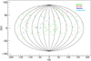 |
Fig. 1. Sky distribution of the sources from our sample and their respective polarization angles measured with respect to the local longitude. |
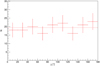 |
Fig. 2. Polarization angle distribution of our sample of 175 AGNs. Both redshift and polarization measurements are available for these AGNs. |
3. Measure of anisotropy
The polarization angles of the AGNs of our sample are on the hypothetical celestial sphere and directional measurement on this sphere corresponds to a particular coordinate system. To test our hypothesis of isotropy, we resort to the coordinate independent statistics procedure of Jain et al. (2004) and compare the polarization vector of a source after transporting it to the position of a reference source along the geodesic joining the two. We define the measure of isotropy according to Hutsemékers (1998) and Jain et al. (2004). We have both redshift and angular position, that is, right ascension and declination, for each source. We define the separation between any two given sources in terms of comoving distance. When calculating comoving distances we assume ΛCDM and cosmological parameters from the latest Planck results (Planck Collaboration 2018). Subsequently, we consider the nv nearest neighbors of a source situated at site k with its polarization angle ψk. We let ψi be the polarization angle of the source at ith site within the nv nearest -neighbor set. A dispersion measure of polarization angles relative to the kth source ψk with its nv nearest neighbor is written as
![Mathematical equation: $$ \begin{aligned} d_{k} = \frac{1}{n_{\rm v}} \mathop \sum \limits _{i=1}^{n_{\rm v}} \cos [2(\psi _{i}+\Delta _{i\rightarrow k}) - 2{\psi }_{k}], \end{aligned} $$](/articles/aa/full_html/2019/02/aa34192-18/aa34192-18-eq1.gif) (1)
(1)
where Δi → k is a correction to angle ψi due to its parallel transport from site i → k (Jain et al. 2004). The polarization angles span a range of 0–180° and to make them behave like usual angles and take values over the entire range of 0–360° we multiply the polarization angles by two (Ralston & Jain 1999). The function dk is the average of the cosine of the differences of the polarization vector at site k and those of its nv nearest-neighbor set and hence is a measure of the dispersion in angles. It takes on higher values for data with lower dispersions and vice versa. We take the average of dk over all source sites and define this as a measure of alignment in our sample:
 (2)
(2)
where Nt is the total number of sources in the sample. Similar alternate statistics can also be defined as a measure of alignment (Bietenholz 1986; Hutsemékers 1998; Jain et al. 2004; Tiwari & Jain 2013; Pelgrims & Cudell 2014). The nearest-neighbor statistics uses the number of nearest neighbors, nv, as a proxy of distance. This is to fix statistics at each source location, i.e., to have the same nv while calculating dk. The average distance corresponding to nv for the different sub-sample studies in this work is given in Fig. 3.
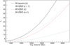 |
Fig. 3. Average distance corresponding to nv. The distance is computed assuming ΛCDM, and the cosmological parameters are taken from the latest Planck results (Planck Collaboration 2018). “All sources (z)” sample contains 175 sources, all with redshifts and good polarization measurements. Of these 175 sources, 139 are quasars; 69 of these quasars are above a redshift of one. |
The error in the statistic SD is computed using the jackknife method (Tiwari & Jain 2016) and the significance is computed by comparing the data SD with a random sample SD. The random sample SD is generated by assigning random polarization angles or random jet angles to each source. The jackknife error on SD for a given nv is calculated by re-sampling the data. We eliminate the ith source from the full sample and calculate the correlation statistics SD(i). Given full-sample statistics SD, the jackknife error δSD in its estimation is given as,
 (3)
(3)
4. Analysis and results
Our full sample contains 211 sources; both redshift and good polarization measurements are available for 175 of these, that is, a good sample for our analysis. There are 183 sources with jet angle measurements along with redshifts. The SD measurements and their significance as compared to a random sample (“random SD”) are shown in Fig. 4. The σ significance, that is, how the sample behaves with respect to random isotropic and uniform polarization angles, is defined as follows,
 (4)
(4)
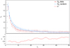 |
Fig. 4. Statistics SD of all sources and its significance with respect to random isotropic polarization distribution. The error bars on our data sample SD are jackknife errors. The random sample SD is also shown with RMS error bars drawn from 1000 random samples. The σ significance is the difference between the data SD and the random SD samples as defined in Eq. (4). |
where  and
and  are jackknife errors on data SD and RMS errors on random
  , respectively. The results with full data in Fig. 4 show no significant deviation from isotropy and are well within one sigma of the isotropic and uniform distribution of polarization angles. The jet angles also show good agreement with random jet angle distribution; results are shown in Fig. 5. The average distance to first nearest neighbor in our full sample is 719 Mpc. Therefore, the observation of isotropy in this work applies for distance scales ≥719 Mpc. We are limited by source number density to probe smaller scales and so cannot explore the polarization angle alignment signal claimed at scales of order 100 Mpc (Tiwari & Jain 2013).
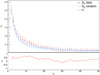 |
Fig. 5. Statistics SD of jet angles. Jet position angles are fairly isotropic and agree well within 1 σ with the random sample. Other details are as in Fig. 4. |
There have been several observations of quasar polarization alignments at large distance scales (Hutsemékers et al. 2014; Pelgrims & Hutsemékers 2015, 2016) and so we also explore the anisotropy in our sample of quasars. There are a total of 139 quasars in our full sample for which we have redshift and polarization angle measurements. These are evenly distributed over the northern sky (Fig. 1) and centered around a redshift of one (see Figs. 2 and 3 in Agudo et al. 2014). Again, we do not see any alignment in this quasar-only sample and the statistics agree well with a random distribution. The results are shown in Fig. 6. The smallest nearest neighbor distance in this sample is 849 Mpc and so the quasar polarization angle distribution is isotropic at least at this scale and above.
Next, we test if the alignment signal is redshift dependent, and whether or not it is present with high-redshift quasars (Pelgrims & Hutsemékers 2015). We consider quasars with redshifts larger than one and calculate SD; this sample contains 67 quasars and for this sample the average distance to first nearest neighbor is 1153 Mpc. We find that this sample also agrees well with a random distribution; no significant alignment is seen. Results are shown in Fig. 7. The quasar sample with redshift less than one is also consistent with isotropic polarization distribution.
5. Discussion and conclusion
The polarization angle alignment of radio sources and quasars at large distance scales continues to puzzle cosmologists and has done for many years now (Birch 1982; Kendall & Young 1984; Hutsemékers 1998; Jain & Ralston 1999; Tiwari & Jain 2013; Hutsemékers et al. 2014; Pelgrims & Hutsemékers 2015, 2016). Surprisingly, most of these, along with CMB dipole-quadrupole-octopole (de Oliveira-Costa et al. 2004; Schwarz et al. 2004), radio galaxy distribution dipole (Singal 2011; Gibelyou & Huterer 2012; Rubart & Schwarz 2013; Tiwari et al. 2015; Tiwari & Jain 2015; Tiwari & Nusser 2016; Colin et al. 2017), and polarizations at optical frequencies at cosmological scale, indicate a preferred direction pointing roughly towards the Virgo cluster (Ralston & Jain 2004). Although there exist some explanations for the large-scale optical polarization alignment following axion-photon interaction (Agarwal et al. 2012), and radio polarization alignment at scales of 150 Mpc in terms of galaxy supercluster magnetic field (Tiwari & Jain 2016), the alignment signal reported by Hutsemékers (1998), Hutsemékers et al. (2014), Pelgrims & Hutsemékers (2015), and Pelgrims & Hutsemékers (2016) remains puzzling. In this work we explore millimeter radio polarization alignment on a large scale and find that our results support isotropy.
The observed isotropy is likely to impose significant constraints on the proposed mechanisms for large-scale polarization alignment discussed in Sect. 1 (Jain et al. 2002; Agarwal et al. 2011, 2012; Piotrovich et al. 2009; Morales & Saez 2007; Urban & Zhitnitsky 2010; Poltis & Stojkovic 2010; Hackmann et al. 2010; Ciarcelluti 2012; Chakrabarty 2016). The constraints may be more stringent on mechanisms which predict an effect independent of frequency or a larger effect at smaller frequency. This is because such models will predict an alignment of the same or higher strength in comparison to that seen at optical frequencies (Hutsemékers 1998). In contrast, the constraints may not be very stringent on pseudoscalar-photon mixing (Jain et al. 2002), for example, which increases with frequency. Many of these mechanisms rely on the presence of large-scale correlated magnetic field. Hence the observed alignment may also be a probe of the correlations in the large-scale magnetic field. However, this relationship between alignment and magnetic field is not direct since it also relies on some other effects, such as the mixing of electromagnetic radiation with hypothetical pseudoscalar particles (Andriamonje et al. 2007; Tiwari 2012, 2017; Payez et al. 2012; Wouters & Brun 2013; Ayala et al. 2014). On small distance scales of the order of 100 Mpc it has been speculated that supercluster magnetic field may directly affect the alignment of galaxies (Tiwari & Jain 2016). However, in this case the alignment effect will also depend on the level of randomness introduced by local effects within individual galaxies.
Earlier studies reporting on the alignment of radio polarization were usually in 2D due to unavailable measurements of redshift. Therefore, to test if the alignment signal was a consequence of 2D projection, we calculate SD for our sample at fixed redshift, that is, projecting all sources at the same redshift. Even with 2D statistics we find the samples (both the full and quasar-only samples) to agree well with random a distribution (Fig. 8).
We also test the data with alternate statistics. In particularly we test the data by averaging SD at a fixed distance, that is, averaging dispersion over the spheres of fixed radii at each site. This also closely matches with random isotropic polarization distribution. Results are shown in Fig. 9. Furthermore, the high-redshift quasar distribution is also isotropic.
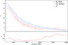 |
Fig. 9. Alignment at fixed distance. SD is the average dispersion over the spheres of radius “Distance” on the x-axis at each source site. The number of nearest neighbor nv at each site varies here slightly. Other details are as in Fig. 4. |
We have tested the large-scale radio polarization alignment signal with a robust and simultaneous dual-frequency radio polarimetric survey (Agudo et al. 2014). We do not find any observation of alignment at a large scale. Furthermore, we find polarization angles of AGNs and jet angles to be relatively uniform and isotropic at scales equal to and greater than ∼1 Gpc. However, due to low number density, we are unable to probe scales less than 719 Mpc and cannot examine the alignment claimed at smaller scales (Tiwari & Jain 2013; Jagannathan & Taylor 2014). Furthermore, with this sample we cannot explore the alignment with the axis of large quasar groups (LQGs; Pelgrims & Hutsemékers 2016). This is because the LQGs are typically of smaller size in comparison to the distance scale of the first neighbor in our sample.
We note that the jet position angles with respect to the polarization angles in our sample of AGNs are not preferentially parallel or perpendicular (Agudo et al. 2014). This is somewhat unusual and unlike the predictions from axially symmetric jet models (Falle 1991; Martí et al. 1997; Komissarov 1999; Fendt et al. 2012) and probably indicates that the magnetic field or the particles in the radio emission region are nonaxisymmetric and that somehow due to local magnetic fields or other effects the polarization vector is misaligned with respect to jet position angle. However, this observation does not change our conclusions as we find isotropy with jet position angle as well.
Nevertheless, this work adds to the previous studies of large-scale radio polarization alignment anomalies. With this data we clearly see the isotropy on scales above 1 Gpc. These results further support the isotropy assumption in cosmology along with CMB and other observations supporting large-scale isotropy.
Acknowledgments
This work is supported by NSFC Grants 1171001024 and 11673025, the National Key Basic Research and Development Program of China (No. 2018YFA0404503) and the Science and Engineering Research Board (SERB), Government of India. The work is also supported by NAOC youth talent fund 110000JJ01.
References
- Abu-Zayyad, T., Aida, R., Allen, M., et al. 2012, ApJ, 757, 26 [Google Scholar]
- Agarwal, N., Kamal, A., & Jain, P. 2011, Phys. Rev. D, 83, 065014 [NASA ADS] [CrossRef] [Google Scholar]
- Agarwal, N., Aluri, P. K., Jain, P., Khanna, U., & Tiwari, P. 2012, EPJC, 72, 15 [Google Scholar]
- Agudo, I., Thum, C., Wiesemeyer, H., & Krichbaum, T. P. 2010, ApJS, 189, 1 [NASA ADS] [CrossRef] [Google Scholar]
- Agudo, I., Thum, C., Gómez, J. L., & Wiesemeyer, H. 2014, A&A, 566, A59 [NASA ADS] [CrossRef] [EDP Sciences] [Google Scholar]
- Aluri, P. K., Ralston, J. P., & Weltman, A. 2017, MNRAS, 472, 2410 [NASA ADS] [CrossRef] [Google Scholar]
- Andriamonje, S., Aune, S., Autiero, D., et al. 2007, JCAP, 4, 010 [NASA ADS] [CrossRef] [Google Scholar]
- Ayala, A., Domínguez, I., Giannotti, M., Mirizzi, A., & Straniero, O. 2014, Phys. Rev. Lett., 113, 191302 [NASA ADS] [CrossRef] [Google Scholar]
- Bennett, C. L., Larson, D., Weiland, J. L., et al. 2013, ApJS, 208, 20 [Google Scholar]
- Bietenholz, M. F. 1986, AJ, 91, 1249 [NASA ADS] [CrossRef] [Google Scholar]
- Birch, P. 1982, Nature, 298, 451 [NASA ADS] [CrossRef] [Google Scholar]
- Chakrabarty, S. S. 2016, Phys. Rev. D, 93, 123507 [NASA ADS] [CrossRef] [Google Scholar]
- Ciarcelluti, P. 2012, Mod. Phys. Lett. A, 27, 1250221 [NASA ADS] [CrossRef] [Google Scholar]
- Colin, J., Mohayaee, R., Rameez, M., & Sarkar, S. 2017, MNRAS, 471, 1045 [NASA ADS] [CrossRef] [Google Scholar]
- de Oliveira-Costa, A., Tegmark, M., Zaldarriaga, M., & Hamilton, A. 2004, Phys. Rev. D, 69, 063516 [NASA ADS] [CrossRef] [Google Scholar]
- Falle, S. A. E. G. 1991, MNRAS, 250, 581 [NASA ADS] [CrossRef] [Google Scholar]
- Fendt, C., Porth, O., & Vaidya, B. 2012, J. Phys. Conf. Ser., 372, 012011 [CrossRef] [Google Scholar]
- Gibelyou, C., & Huterer, D. 2012, MNRAS, 427, 1994 [NASA ADS] [CrossRef] [Google Scholar]
- Hackmann, E., Hartmann, B., Lammerzahl, C., & Sirimachan, P. 2010, Phys. Rev. D, 82, 044024 [NASA ADS] [CrossRef] [Google Scholar]
- Hutsemékers, D. 1998, A&A, 332, 410 [NASA ADS] [Google Scholar]
- Hutsemékers, D., Braibant, L., Pelgrims, V., & Sluse, D. 2014, A&A, 572, A18 [NASA ADS] [CrossRef] [EDP Sciences] [Google Scholar]
- Jackson, N., Battye, R., Browne, I., et al. 2007, MNRAS, 376, 371 [NASA ADS] [CrossRef] [Google Scholar]
- Jagannathan, P., & Taylor, R. 2014, AAS Meeting Abst., 223, 150.34 [Google Scholar]
- Jain, P., & Ralston, J. P. 1999, Mod. Phys. Lett. A, 14, 417 [NASA ADS] [CrossRef] [Google Scholar]
- Jain, P., Panda, S., & Sarala, S. 2002, Phys. Rev. D, 66, 085007 [NASA ADS] [CrossRef] [Google Scholar]
- Jain, P., Narain, G., & Sarala, S. 2004, MNRAS, 347, 394 [NASA ADS] [CrossRef] [Google Scholar]
- Joshi, S., Battye, R., Browne, I., et al. 2007, MNRAS, 380, 162 [NASA ADS] [CrossRef] [Google Scholar]
- Kendall, D. G., & Young, G. A. 1984, MNRAS, 207, 637 [NASA ADS] [CrossRef] [Google Scholar]
- Komissarov, S. S. 1999, MNRAS, 308, 1069 [NASA ADS] [CrossRef] [Google Scholar]
- Martí, J. M., Müller, E., Font, J. A., Ibáñez, J. M. Z., & Marquina, A. 1997, ApJ, 479, 151 [NASA ADS] [CrossRef] [Google Scholar]
- Milne, E. A. 1933, Z. Astrophys., 6, 1 [NASA ADS] [Google Scholar]
- Milne, E. A. 1935, Relativity, gravitation and world-structure (Oxford: The Clarendon press) [Google Scholar]
- Morales, J. A., & Saez, D. 2007, Phys. Rev. D, 75, 043011 [NASA ADS] [CrossRef] [Google Scholar]
- Payez, A., Cudell, J., & Hutsemekers, D. 2012, JCAP, 1207, 041 [NASA ADS] [CrossRef] [Google Scholar]
- Pelgrims, V., & Cudell, J. R. 2014, MNRAS, 442, 1239 [NASA ADS] [CrossRef] [Google Scholar]
- Pelgrims, V., & Hutsemékers, D. 2015, MNRAS, 450, 4161 [NASA ADS] [CrossRef] [Google Scholar]
- Pelgrims, V., & Hutsemékers, D. 2016, A&A, 590, A53 [NASA ADS] [CrossRef] [EDP Sciences] [Google Scholar]
- Penzias, A. A., & Wilson, R. W. 1965, ApJ, 142, 419 [NASA ADS] [CrossRef] [Google Scholar]
- Piotrovich, M Yu, Gnedin, Yu N, & Natsvlishvili, T. M. 2009, Astrophysics, 52, 451 [CrossRef] [Google Scholar]
- Planck Collaboration XVI. 2016, A&A, 594, A16 [NASA ADS] [CrossRef] [EDP Sciences] [Google Scholar]
- Planck Collaboration 2018, A&A, submitted [arXiv:1807.06209] [Google Scholar]
- Poltis, R., & Stojkovic, D. 2010, Phys. Rev. Lett., 105, 161301 [NASA ADS] [CrossRef] [Google Scholar]
- Ralston, J. P., & Jain, P. 1999, IJMPD, 8, 537 [NASA ADS] [CrossRef] [Google Scholar]
- Ralston, J. P., & Jain, P. 2004, IJMPD, 13, 1857 [NASA ADS] [CrossRef] [Google Scholar]
- Rath, P. K., Samal, P. K., Panda, S., & Mishra, D. D. 2018, MNRAS, 475, 4357 [NASA ADS] [CrossRef] [Google Scholar]
- Řípa, J., & Shafieloo, A. 2017, ApJ, 851, 15 [NASA ADS] [CrossRef] [Google Scholar]
- Rubart, M., & Schwarz, D. J. 2013, A&A, 555, A117 [NASA ADS] [CrossRef] [EDP Sciences] [Google Scholar]
- Schwarz, D. J., Starkman, G. D., Huterer, D., & Copi, C. J. 2004, Phys. Rev. Lett., 93, 221301 [NASA ADS] [CrossRef] [PubMed] [Google Scholar]
- Schwarz, D. J., Copi, C. J., Huterer, D., & Starkman, G. D. 2016, Class. Quant. Grav., 33, 184001 [NASA ADS] [CrossRef] [Google Scholar]
- Shurtleff, R. 2014, ArXiv eprints [arXiv:1408.2514] [Google Scholar]
- Singal, A. K. 2011, ApJ, 742, L23 [NASA ADS] [CrossRef] [Google Scholar]
- Thum, C., Wiesemeyer, H., Paubert, G., Navarro, S., & Morris, D. 2008, PASP, 120, 777 [NASA ADS] [CrossRef] [Google Scholar]
- Tiwari, P. 2012, Phys. Rev. D, 86, 115025 [NASA ADS] [CrossRef] [Google Scholar]
- Tiwari, P. 2017, Phys. Rev. D, 95, 023005 [NASA ADS] [CrossRef] [Google Scholar]
- Tiwari, P., & Jain, P. 2013, Int. J. Mod. Phys., D, 22, 1350089 [NASA ADS] [CrossRef] [Google Scholar]
- Tiwari, P., & Jain, P. 2015, MNRAS, 447, 2658 [NASA ADS] [CrossRef] [Google Scholar]
- Tiwari, P., & Jain, P. 2016, MNRAS, 460, 2698 [NASA ADS] [CrossRef] [Google Scholar]
- Tiwari, P., & Nusser, A. 2016, JCAP, 2016, 062 [Google Scholar]
- Tiwari, P., Kothari, R., Naskar, A., Nadkarni-Ghosh, S., & Jain, P. 2015, Astropart. Phys., 61, 1 [NASA ADS] [CrossRef] [Google Scholar]
- Urban, F. R., & Zhitnitsky, A. R. 2010, Phys. Rev. D, 82, 043524 [NASA ADS] [CrossRef] [Google Scholar]
- White, M., Scott, D., & Silk, J. 1994, ARA&A, 32, 319 [NASA ADS] [CrossRef] [Google Scholar]
- Wouters, D., & Brun, P. 2013, ApJ, 772, 44 [NASA ADS] [CrossRef] [Google Scholar]
- Zavala, R. T., & Taylor, G. B. 2004, ApJ, 612, 749 [NASA ADS] [CrossRef] [Google Scholar]
All Figures
|
Fig. 1. Sky distribution of the sources from our sample and their respective polarization angles measured with respect to the local longitude. |
| In the text | |
|
Fig. 2. Polarization angle distribution of our sample of 175 AGNs. Both redshift and polarization measurements are available for these AGNs. |
| In the text | |
|
Fig. 3. Average distance corresponding to nv. The distance is computed assuming ΛCDM, and the cosmological parameters are taken from the latest Planck results (Planck Collaboration 2018). “All sources (z)” sample contains 175 sources, all with redshifts and good polarization measurements. Of these 175 sources, 139 are quasars; 69 of these quasars are above a redshift of one. |
| In the text | |
|
Fig. 4. Statistics SD of all sources and its significance with respect to random isotropic polarization distribution. The error bars on our data sample SD are jackknife errors. The random sample SD is also shown with RMS error bars drawn from 1000 random samples. The σ significance is the difference between the data SD and the random SD samples as defined in Eq. (4). |
| In the text | |
|
Fig. 5. Statistics SD of jet angles. Jet position angles are fairly isotropic and agree well within 1 σ with the random sample. Other details are as in Fig. 4. |
| In the text | |
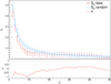 |
Fig. 6. Statistics SD exclusive to our sample of 139 quasars. Other details are as in Fig. 4. |
| In the text | |
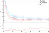 |
Fig. 7. Quasars from our sample with redshift greater than one. Other details are as in Fig. 4. |
| In the text | |
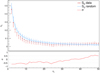 |
Fig. 8. Statistics SD calculated with a 2D sample. Other details are as in Fig. 4. |
| In the text | |
|
Fig. 9. Alignment at fixed distance. SD is the average dispersion over the spheres of radius “Distance” on the x-axis at each source site. The number of nearest neighbor nv at each site varies here slightly. Other details are as in Fig. 4. |
| In the text | |
Current usage metrics show cumulative count of Article Views (full-text article views including HTML views, PDF and ePub downloads, according to the available data) and Abstracts Views on Vision4Press platform.
Data correspond to usage on the plateform after 2015. The current usage metrics is available 48-96 hours after online publication and is updated daily on week days.
Initial download of the metrics may take a while.