| Issue |
A&A
Volume 622, February 2019
|
|
|---|---|---|
| Article Number | A36 | |
| Number of page(s) | 14 | |
| Section | The Sun | |
| DOI | https://doi.org/10.1051/0004-6361/201833379 | |
| Published online | 24 January 2019 | |
The potential of many-line inversions of photospheric spectropolarimetric data in the visible and near UV
1
Max-Planck-Institut für Sonnensystemforschung (MPS), Justus-von-Liebig-Weg 3, 37077 Göttingen, Germany
e-mail: This email address is being protected from spambots. You need JavaScript enabled to view it.
2
School of Space Research, Kyung Hee University, Yongin, Gyeonggi 446-701, Republic of Korea
Received:
7
May
2018
Accepted:
8
December
2018
Abstract
Our knowledge of the lower solar atmosphere is mainly obtained from spectropolarimetric observations, which are often carried out in the red or infrared spectral range and almost always cover only a single or a few spectral lines. Here we compare the quality of Stokes inversions of only a few spectral lines with many-line inversions. In connection with this, we have also investigated the feasibility of spectropolarimetry in the short-wavelength range, 3000 Å−4300 Å, where the line density but also the photon noise are considerably higher than in the red, so that many-line inversions could be particularly attractive in that wavelength range. This is also timely because this wavelength range will be the focus of a new spectropolarimeter in the third science flight of the balloon-borne solar observatory SUNRISE. For an ensemble of state-of-the-art magneto-hydrodynamical atmospheres we synthesize exemplarily spectral regions around 3140 Å (containing 371 identified spectral lines), around 4080 Å (328 lines), and around 6302 Å (110 lines). The spectral coverage is chosen such that at a spectral resolving power of 150 000 the spectra can be recorded by a 2K × 2K detector. The synthetic Stokes profiles are degraded with a typical photon noise and afterward inverted. The atmospheric parameters of the inversion of noisy profiles are compared with the inversion of noise-free spectra. We find that significantly more information can be obtained from many-line inversions than from a traditionally used inversion of only a few spectral lines. We further find that information on the upper photosphere can be significantly more reliably obtained at short wavelengths. In the mid and lower photosphere, the many-line approach at 4080 Å provides equally good results as the many-line approach at 6302 Å for the magnetic field strength and the line-of-sight (LOS) velocity, while the temperature determination is even more precise by a factor of three. We conclude from our results that many-line spectropolarimetry should be the preferred option in the future, and in particular at short wavelengths it offers a high potential in solar physics.
Key words: Sun: magnetic fields / Sun: photosphere / magnetohydrodynamics (MHD)
© ESO 2019
1. Introduction
Gaining knowledge about the solar atmosphere requires the determination of its physical parameters such as temperature (T), magnetic field strength (B), magnetic field inclination (γ), magnetic field azimuth (ϕ), and line-of-sight velocity (vLOS). This is preferably achieved by Stokes inversions (see the recent review by del Toro Iniesta & Ruiz Cobo 2016) of observational data recorded with spectropolarimeters, most of which can be classified as either imaging spectropolarimeters (ISPs), or slit spectropolarimeters (SSPs).
To allow the investigation of dynamic processes, ISPs are mostly used at high cadences at the price of an only modest spectral resolution and spectral coverage. The opposite is true for SSPs. It is only natural that most ISPs record only a few spectral lines because the wavelength interval is scanned by tuning a variable filter, which usually takes time and significantly influences the cadence. Examples of ISPs are the instruments CRISP at the Swedish Solar Telescope (Scharmer 2006), IBIS at the Dunn Solar Telescope (Cavallini 2006), IMaX onboard the balloon-borne SUNRISE observatory (Martínez Pillet et al. 2011), NFI onboard the Hinode satellite (Tsuneta et al. 2008), or HMI onboard the Solar Dynamics Observatory (Scherrer et al. 2012).
An SSP records the spectrum at a slit position quasi instantaneously. The number of spectral lines then only depends on the wavelength, the spectral resolution, and the size of the detector, meaning that theoretically the recording of many spectral lines has long been possible. Numerous studies employing many spectral lines have been carried out in the past, in particular using data gathered with a Fourier Transform Spectrometer (FTS; Brault 1978), for example Stenflo et al. (1983, 1984), Balthasar (1984), Solanki & Stenflo (1984, 1985), and Solanki et al. (1986). However, more recently, observations of the solar photosphere at high spatial resolution are almost entirely carried out with only a few spectral lines. Prominent examples are the instruments SP onboard the Hinode satellite (Lites et al. 2013), Trippel at the Swedish Solar Telescope (Kiselman et al. 2011), TIP2 at the Vacuum Tower Telescope (Collados et al. 2007), and GRIS at the GREGOR Solar Telescope (Collados et al. 2012).
Reasons for this limitation to a few spectral lines are, firstly, that the photon flux available for ground-based observations is decreased by the higher scattering of the blue part of sunlight in the Earth’s atmosphere. Secondly, there is a focus on isolated (i.e., not blended) spectral lines with a clear continuum, which are preferably found in the red and infrared spectral range. Only then is the use of classical methods of estimating atmospheric parameters directly from the Stokes profiles possible (see Solanki 1993, for an overview of such techniques), and also the usage of modern Stokes inversion codes is easier. Thirdly, rapid scanning of the evolving solar scene requires rapid read out, which can be achieved by limiting the wavelength range. Fourthly, in the case of satellite-based instruments, limitations of the telemetry bandwidth can also provide a reason for a reduced spectral coverage.
Because a larger number of spectral lines potentially carries more information about the solar atmosphere and because of the improved technical possibilities, increased attention has been paid to many-line approaches in recent times (e.g., Beck 2011; Rezaei & Beck 2015; Quintero Noda et al. 2017a,b). Even observing many similar spectral lines can be helpful in increasing the effective signal-to-noise ratio (S/N) without increasing the integration time, as has been demonstrated in cool-star research (Donati et al. 1997).
By means of an ensemble of magneto-hydrodynamical (MHD) atmospheres, this paper considers quantitatively how well the many-line approach works and how large its advantages (if any) are relative to traditionally used few-line approaches. By way of an example, we carry out our analysis for one spectral region each in the red, in the violet, and in the near ultraviolet (NUV) and compare these. The examples are of general interest, but are chosen specifically to be also of relevance for a new SSP, namely the SUNRISE Ultraviolet Spectropolarimeter and Imager (SUSI). It is planned to operate SUSI onboard the balloon-borne solar observatory SUNRISE (Barthol et al. 2011; Solanki et al. 2010, 2017) during its third science flight at a float altitude above 30 km, so that access to the NUV is possible and the scattering issue in the Earth’s atmosphere does not exist. However, the analysis is general and its applications are not limited to a particular instrument.
In Sect. 2 we present the method and introduce the employed MHD simulation as well as the spectral synthesis. Section 3 describes our results and in Sect. 4 we summarize the study and draw conclusions.
2. Method
We first considered the wavelength region 6280 Å−6323 Å. We chose this wavelength band because it contains the well-studied and frequently used Fe I line pair at 6302 Å that shows strong polarization signals and can be seen as a good example for Stokes inversions of spectropolarimetric data in the red spectral range. The width of the wavelength range is chosen such that it can be critically sampled by a 2K × 2K pixels detector of an SSP at a spectral resolving power of 150 000 (i.e., each pixel covers 0.5λ/150 000), which we considered to be a reasonable compromise between a good spectral resolution and a broad spectral coverage.
A three-dimensional (3D) MHD simulation of the photosphere and upper convection zone, which contains quiet-Sun regions (granulation) as well as strong-field features (pores, bright points), was used for a spectral synthesis of the considered spectral region. After an estimation of the photon budget of a possible state-of-the-art SSP, the synthetic Stokes profiles were degraded with photon noise. Among other tests, we then inverted the degraded synthetic spectra in order to retrieve the atmospheric parameters.
The deviation of the inverted noise-contaminated atmospheres from the inverted noise-free atmospheres indicates how accurate the determination of temperature, magnetic field vector, and LOS velocity in the photosphere is for the considered spectral region. The spectral range in the red was analyzed twice. Firstly, for the many-line approach, that is for the full spectral region fitting on a 2K detector and containing 110 identified spectral lines, and secondly, for a reduced spectral region (6300.8 Å−6303.2 Å) that only covers the traditionally used Fe I 6302 Å line pair.
2.1. MHD simulation
Realistic simulations of the radiative and MHD processes in the photosphere and upper convection zone were carried out with the 3D non-ideal compressible MHD code MURaM (The Max Planck Institute for Solar System Research/University of Chicago Radiation Magneto-hydrodynamics code; see Vögler et al. 2005) that includes non-gray radiative energy transfer under the assumption of local thermal equilibrium (LTE). Our simulation box covers 33.8 Mm × 33.8 Mm in its horizontal dimensions and is 6.1 Mm deep. The τ = 1 surface for the continuum at 5000 Å was on average reached about 700 km below the upper boundary. The cell size of the simulation box is 20.83 km in the two horizontal directions and 16 km in the vertical direction.
At the bottom boundary of the simulation box a free in- and outflow of matter was allowed under the constraint of total mass conservation, while the top boundary was closed (zero vertical velocities). In the horizontal directions we used periodic boundary conditions.
A spectropolarimetric observation of active region AR 11768 (with cosine of the heliocentric angle μ = 0.93), recorded on 2013 June 12, 23:39 UT with the Imaging Magnetograph eXperiment (IMaX; Martínez Pillet et al. 2011) onboard the SUNRISE observatory (Solanki et al. 2010, 2017; Barthol et al. 2011; Berkefeld et al. 2011; Gandorfer et al. 2011), was inverted with the MHD-Assisted Stokes Inversion technique (MASI; Riethmüller et al. 2017). This technique searches an archive of realistically degraded synthetic Stokes profiles for the best matches with the observed profiles. The best-fit MHD atmospheres are used as the initial condition of our simulation. The simulation was then run for a further 54 min of solar time to reach a statistically relaxed state. This study uses a snapshot taken at this time. Figure 1 shows the map of bolometric intensities of the simulation snapshot. To limit the computational effort needed for the current study we limited our analysis to the 3.0 Mm × 3.3 Mm wide region of interest indicated by the white box “A” in Fig. 1, which, in spite of its small size, contains part of a pore, some bright points, and seemingly normal granulation.
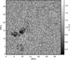 |
Fig. 1. Bolometric intensity image of the used MURaM simulation snapshot. The white boxes labeled with “A” and “B” indicate the regions of interest employed in this study. |
2.2. Spectral synthesis
To obtain synthetic Stokes spectra from the MURaM simulation we used the inversion code SPINOR (Stokes-Profiles-INversion-O-Routines; see Frutiger et al. 2000) in its forward calculation mode. This code incorporates the STOPRO (STOkes PROfiles) routines (Solanki 1987), which compute synthetic Stokes profiles of one or more spectral lines upon input of their atomic or molecular data and a model atmosphere. LTE conditions are assumed and the Unno-Rachkovsky radiative transfer equations (Rachkovsky 1962) are solved. All spectral line syntheses in this paper were carried out for the center of the solar disk ( μ = 1).
We downloaded the atomic data of all spectral lines found in the atomic line databases of Kurucz (Kurucz & Bell 1995) and VALD (Vienna Atomic Line Database; see Ryabchikova et al. 2015) for the considered wavelength ranges. We performed a test-wise synthesis for every single line contained in these databases for a hot standard atmosphere, the HSRA (Chapman 1979) extended to deeper layers representing the quiet Sun, and also for a cold standard atmosphere, the Maltby-M (Maltby et al. 1986) representing the core of an umbra. For these test computations we assigned a zero velocity and magnetic field to the atmospheres. We ignored all spectral lines that could not be synthesized with SPINOR due to its limitations (e.g., SPINOR only supports neutral and singly ionized atoms/molecules but no higher ionization states) and from the synthesizeable lines we further ignored insignificant ones in the sense that we only considered spectral lines with a line depth larger than 10−2 in units of the continuum intensity in either of the two standard atmospheres. By applying this procedure we identified 110 atomic lines for the 6280 Å−6323 Å spectral region. The solar abundance of all elements, including carbon, nitrogen, and oxygen, was taken from Grevesse & Sauval (1998).
The 110 spectral lines that where found synthesizeable by SPINOR and relevant for the solar photosphere were then synthesized again for an HSRA temperature stratification and a zero velocity, but this time we assigned a magnetic field of 1 kG strength and 30° inclination. The magnetic field properties of the atmosphere were taken to be constant with height and were selected such that significant polarization signals in Stokes Q, U, and V are reached. Also, after the radiative transfer computation, we spectrally degraded the Stokes profiles to a spectral resolving power of 150 000. The corresponding Stokes spectra are plotted in Fig. 2. This spectral region contains the Fe I 6301.5 Å and 6302.5 Å line pair, which is well studied, for example via the spectropolarimeter onboard the Hinode satellite (Tsuneta et al. 2008; Lites et al. 2013). The amplitudes of the synthetic Stokes V signal of the two Fe I lines are 18.9% and 26.9%, respectively, while the amplitudes of the linear polarization ( ) signal are 1.6% and 3.5%.
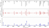 |
Fig. 2. Synthetic Stokes I (black line), Stokes V (red line), and linear polarization (blue line) profile at a spectral resolution of 150 000 for a wavelength region around 6302 Å chosen to fit on a 2048 pixel wide detector if critically sampled in the wavelength domain. All spectra are normalized to the mean quiet-Sun intensity, IQS. The horizontal lines in the lower two panels mark polarization levels of 10, 20, 30% for Stokes V and 1, 2, 3, 4, 5% for the linear polarization. Spectral lines providing |V| > 20% are labeled with the element forming the line. |
2.3. Photon noise
Because the photon noise is calculated from the square root of the number of photo electrons, we compiled the photon budget of a state-of-the-art slit spectropolarimeter in Table 1. As an example, the used instrument parameters are based on the planned SUNRISE/SUSI instrument. We started our calculation with the solar spectral irradiance, Is, which was measured by the third ATmospheric Laboratory for Application and Science mission (ATLAS 3; Thuillier et al. 2004, 2014). Since Is is the photon flux of the Sun integrated over the entire solar disk, we had to divide by the wavelength dependent limb-darkening factor in order to get the photon flux at disk center (DC).
Photon budget for the mean quiet-Sun intensity at disk center at the three wavelengths under study.
Parameters that can be influenced by the design of SUNRISE/SUSI are the pixel size, the spectral resolution, the total transmission of the telescope and the instrument, the quantum efficiency of the camera, the total integration time of the observation, and the polarimetric efficiency.
In the calculations an arc-second is fixed at 736.4 km and the solar radius at 944.93421 arcsec, which corresponds to an observation time of mid June, which is typical for a SUNRISE flight in the Arctic. The primary mirror of the SUNRISE telescope has a diameter of 100 cm and its central obscuration is 23.2 cm across.
A cutting-edge SSP design includes a strictly synchronized, broadband slit-jaw camera that allows the determination of the point spread function (PSF). The PSF can then be used to reconstruct the spectral data (van Noort 2017) to correct for the residual wavefront aberrations. We expect an increase in noise by the spectral restoration and took this into account in our photon budget by the noise amplification factor, a.
The calculation of the photon noise for the wavelength range centered on 6302 Å can be found in the third column of Table 1, while the fourth and fifth column show the calculation for the wavelength bands around 4080 Å and 3140 Å that we will consider later in Sect. 3.2.
2.4. Stokes inversion
After degrading the synthetic Stokes profiles with photon noise according to Table 1, the atmospheric parameters were retrieved from Stokes inversions. For this step the SPINOR code was used in its inversion mode. We applied an atmospheric model with five optical depth nodes at log τ = −4, −2.5, −1.5, −0.8, 0 for T, B, γ, ϕ, and vLOS, as well as a height-independent micro turbulence. All wavelengths were weighted equally. The synthetic Stokes spectra that were calculated during the inversion were always convolved with a Gaussian profile that corresponds to a spectral resolving power of 150 000.
The SPINOR inversion code was run twice in a row with 100 iterations each. While the first inversion run was carried out with uniform initial conditions, a second run used the spatially smoothed inversion result of the first run as the initial guess atmosphere. This procedure removed spatial discontinuities in the physical quantities that can occur if the inversion gets stuck in local minima of the merit function at individual pixels or groups of pixels (see also Kahil et al. 2017; Solanki et al. 2017).
3. Results
An ensemble of physically consistent MHD atmospheres of the region enclosed by the white box “A” in Fig. 1 covers important photospheric features (quiet Sun, pores, bright points) and was used for the statistical analysis in this work. All relevant spectral lines in the considered wavelength region were synthesized for this ensemble of atmospheres. The computed Stokes spectra were spectrally degraded to a spectral resolving power of 150 000 and the expected photon noise was added as given in Table 1. The noisy Stokes spectra were inverted with the SPINOR code and the obtained atmospheric parameters were then compared with the inverted quantities of the noise-free spectra.
For each atmospheric parameter and each optical depth node we subtract the maps of the noisy inversion from the noise-free inversion and calculate the standard deviation, σ, over all pixels of such a difference image. In this way the inversion error purely induced by the noise can be expressed in the form of a single number.
3.1. Comparison of the many-line approach to the double-line approach in the red
Table 2 lists the inversion errors induced by photon noise for the many-line approach at 6302 Å, that is for the spectral region 6280 Å−6323 Å containing 110 considered spectral lines. We compare the many-line inversion with the same type of inversion restricted to only two spectral lines (6300.8 Å−6303.2 Å), that is the double-line approach, see Table 3. The comparison strikingly shows the advantage of considering as many spectral lines as possible compared to a generally used single or double-line inversion. T as well as B and vLOS can be determined much better from the noisy Stokes profiles if all the lines are employed. Even for the magnetic field inclination the many-line approach provides slightly better results. Since the computational effort of an inversion is influenced by the number of the considered spectral lines, the many-line inversion consumes 22 times more computation time than the double-line approach, if all other inversion parameters are kept the same.
For both approaches, the temperature is best determined at log τ = 0, as expected. There the temperature can be retrieved from noisy Stokes profiles by a factor of almost seven more accurate if the entire spectral region is considered instead of only the one limited to the Fe I line pair. B and vLOS are formed slightly higher in the solar atmosphere, so that we find the smallest uncertainty at log τ = −0.8, where the accuracy of both quantities increases by a factor of roughly two by using all spectral lines fitting on a 2K detector.
Generally, the σ values in the upper photosphere (at log τ = −4) are larger than lower down in the atmosphere. Since this is particularly true for the double-line approach, we consider if this is caused by the fact that spectra limited to only two spectral lines do not provide enough information for five optical depth nodes or, alternatively, if none of the spectral lines from the chosen spectral range in the red provides information about the upper photosphere. To shed some light on this matter, we simplified our inversion model for the double-line inversion to only four optical depth nodes at log τ = −2.5, −1.5, −0.8, 0 (see Table 4) and, even more restrictively, to only three optical depth nodes at log τ = −2.5, −1, 0 (see Table 5), while all other inversion parameters remained unchanged.
The reduction of the number of nodes leads to significantly more accurate T values at all considered optical depths (at the price of a reduced knowledge of the height dependence), while we find an ambiguous picture for B. At log τ = −1, the standard deviation of B is only half of the corresponding value for the five-node inversion (log τ = −0.8) at the expense of worse results for B somewhat higher up at log τ = −2.5. For vLOS we find a slight improvement when reducing the number of nodes from five to four, but for the three-node inversion the situation is similar to the one for B.
To limit the computational effort, we so far considered only a relatively small region of interest (white box labeled with “A” in Fig. 1). We now test the statistical significance of our analysis by repeating the many-line inversion at 6302 Å for another region of almost the same size (box “B” in Fig. 1). The standard deviations are listed in Table 6 and show almost identical values for the temperature and also for the magnetic field inclination. The values for B and vLOS seem to be better determined for region “B”, probably because this is a pure quiet-Sun region that does not contain any dark strong-field features as we have in region “A”. The S/N of such dark features can be much worse than for quite-Sun regions which reduces the accuracy of the retrieved atmospheric quantities.
3.2. Comparison between the red and (ultra)violet spectral bands
The Planck function falls steeply toward short wavelengths, so that spectropolarimetric measurements in the NUV always suffer from the problem of high photon noise relative to the signal. At the same time the spectral line density increases strongly in the NUV. We showed in Sect. 3.1 that the quality of the inversion results in the red spectral range improves significantly if we consider 110 spectral lines instead of only two. Based on that result, we now investigate to what extent the loss of information caused by high photon noise can be compensated by the gain in information due to an increased number of the observed spectral lines. Other effects that also can influence the quality of spectropolarimetric observations, for example stray light, wavefront aberrations, or the wavelength dependence of the diffraction limit are again not considered.
To identify interesting spectral regions in the violet and NUV spectral range, we once more calculated synthetic Stokes profiles for the 1 kG HSRA atmosphere described in Sect. 2.2. We did this for the spectral range 3000 Å−4300 Å that will be covered by the planned slit spectropolarimeter, SUSI, which is to partake on the third science flight of SUNRISE. In addition to the atomic lines of the Kurucz and VALD databases, we also considered some important molecular lines that were identified in previous studies, in particular 139 lines formed by the OH molecule in the spectral region around 3120 Å and 233 lines of the CN molecule around 3880 Å (for details see Riethmüller et al. 2014) as well as 241 CH lines in the so-called G-band, a spectral region around 4300 Å (Shelyag et al. 2004; Riethmüller & Solanki 2017).
We searched the wavelength range 3000 Å−4300 Å for spectral regions fitting on a 2K detector at a critical sampling in the wavelength dimension and exhibiting as many strongly polarized spectral lines as possible. We found several such spectral regions, but limit our study to two of them due to the large computational effort. In the following we focus on the spectral region 3128.5 Å−3150 Å, which is relatively close to the lower wavelength limit of SUSI and hence can potentially provide the highest spatial resolution. At the same time, however, we expect the largest problems with photon noise in this spectral region. Figure 3 shows the synthetic Stokes profiles of this spectral region. 42 of the 371 synthesized spectral lines show a Stokes V signal larger than 10%. Three of them provide a Stokes V signal even larger than 20% and are listed with their Landé factors in Table 7 and, in addition, they are labeled in the middle panel of Fig. 3. A Plin signal higher than 1% is reached by nine spectral lines.
Central wavelengths and Landé factors, g, of considered spectral lines providing a Stokes V signal higher than 20%.
The second spectral region we consider is 4065.49 Å−4093.31 Å because between 3000 Å and 4300 Å it hosts the largest number of strongly polarized spectral lines. Since this region is not too far from the upper limit of the SUSI wavelength range, it has the advantage of a much higher photon flux, but at the price of a somewhat worse diffraction limit. We synthesized 328 spectral lines in this part of the spectrum and plotted the Stokes profiles in Fig. 4. We find a similar number of lines exceeding the 10% level in Stokes V as around 3140 Å, but this time seven of them show a Stokes V signal larger than 20%, a much higher fraction than for the 3140 Å region. In addition, two lines display a Plin signal larger than 3%, namely the Mn I 4070.279 Å line and the Fe I 4080.875 Å line (see Table 7 for their Landé factors).
In Table 8 we contrast the number of strongly polarized spectral lines for the three spectral regions under study. Surprisingly, the 4080 Å region contains more lines than the 6302 Å region with polarization signals above a certain level, while the 3140 Å region is more or less comparable to the one at 6302 Å.
Number of spectral lines found in the three considered wavelength bands that have polarization signals higher than the listed levels.
The basic aim of this part of the study is to compare the results of inversions at the three wavelengths. To do this comparison in a fair manner, we model these wavelength bands as if they were observed by a single instrument. As an example we use the parameters of SUNRISE/SUSI (which, however, will not observe at 6300 Å) and take into account the different noise levels at the three wavelengths etc. We do not, however, scale the pixel size or spatial resolution with wavelength, keeping these two the same, so as to be able to compare the capabilities on an equal footing. The pixel size for all three analyzed spectral regions is fixed at 62.5 km (see Table 1), which roughly corresponds to a critical sampling at 6302 Å. This means, that the SUSI data, for which a critical sampling at 3000 Å is planned, are assumed to be binned.
The wavelength bands around 3140 Å and 4080 Å were identically treated as in the red, meaning that the ensemble of MHD atmospheres of the region enclosed by the white box “A” in Fig. 1 was synthesized, spectrally degraded, contaminated with photon noise, and inverted. Differences between the inversion results of noisy and noise-free profiles were used to calculate standard deviations. The hope, that the increased number of considered spectral lines compensates for the larger noise, came from the fact that the photon noise at 3140 Å is higher by a factor of 2.8 than in the red at 6302 Å (Table 1), while the number of spectral lines identified for the 3140 Å region, however, is larger by a factor of 371/110 = 3.4.
The standard deviations of the many-line inversion in the ultraviolet spectral range around 3140 Å with five optical depth nodes are shown in Table 9. The results of this inversion are competitive to the double-line inversion results in the red (Table 3) because they exhibit similarly good results for B and γ, and an outcome for T and vLOS that is better by factors of two to eight. Compared to a many-line inversion in the red (Table 2), T and vLOS can be determined more accurately at 3140 Å, but for B the UV inversion is only more accurate at log τ = −4.
The most reliable determination of the atmospheric parameters is provided by a many-line inversion at 4080 Å (Table 10). All quantities show much lower standard deviations than for a double-line inversion in the red (Table 3). Even compared to a many-line inversion in the red (Table 2), we generally find considerably lower standard deviations at log τ = −4. The other four optical depth nodes provide clearly more accurate T results at 4080 Å, while the determination of B and vLOS is more or less equally good as in the red.
For an overview of the inversion results, which compares the various approaches and optical depths, we divided the standard deviations by the spatial mean of the unsigned quantities to get relative numbers. For the inversions with five optical depth nodes, the relative standard deviations of T, B, and vLOS are plotted in Fig. 5 and show the superiority of the many-line approach (green line) over the double-line approach (red line) in the red. In the upper photosphere at log τ = −4, the gain in information due to the consideration of many spectral lines is particularly strong, but also observations at shorter wavelengths improve the inversion results in the upper photosphere, at least for T and vLOS. If we consider all three atmospheric quantities at all five optical depths nodes, Fig. 5 demonstrates the outstanding results of the many-line approach at 4080 Å compared to the other wavelengths and even more compared with the double-line approach.
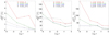 |
Fig. 5. Relative inversion errors as function of the optical depth for the many-line approaches at 3140 Å (black lines), at 4080 Å (blue lines), and at 6302 Å (green lines) as well as for the double-line approach at 6302 Å (red lines). The errors of the three quantities temperature, magnetic field strength and LOS velocity are shown in the left, middle, and right panel, respectively. |
For the many-line inversions in the red, violet, and NUV we used a cluster of 96 cores (AMD Opteron 6176). To invert the Stokes profiles of a single ray in a single inversion run with 100 iterations the mean computational time on this cluster was 85 s at 3140 Å, 20 s at 4080 Å, and 11 s at 6302 Å.
3.3. Scatterplots
Since the standard deviation of a difference image is only a single number that summarizes the deviation of the inversion of noisy spectra from the inversion of noise-free profiles, we now show scatterplots of T, B, and vLOS at the optical depths chosen for the inversion. We do this for two examples of particular interest. First for the many-line approach at 3140 Å, which is the shortest wavelength under study. The five optical depth nodes at log τ = −4, −2.5, −1.5, −0.8, 0 are shown in Fig. 6 from top to bottom (see text labels). The scatter of T and vLOS is relatively low and decreases as the optical depth increases. At optical depth unity, almost no deviations can be found between the results of the noisy and noise-free inversion for T and we see only a small scatter for vLOS. The photon noise causes difficulties, in particular to the determination of B, where the largest deviations from the noise-free inversion are found in the upper atmospheric layers and at higher field strengths. Values greater than B > 2 kG are only reached in pores, where the continuum intensity at 3140 Å can drop to 3.3% of the mean quiet-Sun value, which further reduces the S/N compared to the mean quiet Sun and hence hampers the retrieval of B.
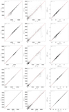 |
Fig. 6. Scatter plots (black dots) of the temperature, magnetic field strength, and LOS velocity (from left to right) retrieved from an inversion of synthetic Stokes profiles degraded with realistic photon noise versus the inversion results from noise-free profiles at the optical depth nodes used during the inversion for the spectral region 3128.5 Å−3150 Å that contains 371 relevant spectral lines. The ideal relation for a perfect fit is indicated by the red line. From top to bottom the panels refer to different optical depth nodes (marked in the figures). |
In our second example we display the scatterplots of the frequently used double-line approach for the spectral region around 6302 Å (Fig. 7). Again, we choose the inversion with five optical depth nodes for a direct comparison with Fig. 6. The T and vLOS values display a considerably larger scatter than at 3140 Å (Fig. 6). Only the scatter in B is approximately equally large, at least for the lower four depth nodes. In the red, the B scatter is not concentrated at strong fields, but is uniformly distributed over the entire B range because the intensity in the pore drops only to 17% (due to the smaller temperature sensitivity of the Planck function in the red part of the spectrum), which leads to a better S/N in the red than in the NUV. In the upper photosphere, at log τ = −4, the scatter of all quantities is by far larger in the red than in the NUV.
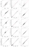 |
Fig. 7. Same as Fig. 6, but for the spectral region 6300.8 Å−6303.2 Å that only contains the Fe I 6301.5 Å and 6302.5 Å line pair. |
3.4. Synthetic spectra versus observed spectra
For a practical application of the many-line approach, not only the trade-off between the photon noise and the number of spectral lines is of importance, but also the following questions play a role: How complete is the list of atomic and molecular spectral lines used for the synthesis and how good is our knowledge of the line parameters (e.g., the oscillator strengths)? In Figs. 8–10 we contrast synthesized spectra with the Jungfraujoch atlas (Delbouille et al. 1973) in order to gain an impression of the completeness and reliability of our syntheses of the solar spectrum. The Jungfraujoch atlas is a spatially averaged spectrum recorded at DC with a spectral resolving power of 216 000 (Doerr et al. 2016). To imitate this, we use a non-gray MURaM simulation box consisting of 288 × 288 × 100 cells each of the size 20 km × 20 km × 16 km with a mean vertical magnetic field strength of 100 G, and calculate a synthetic spectrum for each of the 288 × 288 atmospheres. After a spectral degradation corresponding to a resolving power of 216 000, a spatial averaging of all spectra provides the red lines in Figs. 8–10. The fact that a simulation with a relatively strong mean field provides a good fit, suggests that the Jungfraujoch atlas sampled enhanced network, in addition to quiet Sun (at least at some wavelengths).
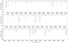 |
Fig. 8. Excerpts from the Jungfraujoch atlas (solar lines in black color, telluric lines in gray color) and from spatially averaged synthetic spectra (red lines; see main text for details). |
Figure 8 compares the Jungfraujoch atlas with the mean synthetic Stokes I profile for the wavelength region 6280 Å−6323 Å. Many spectral lines can be reproduced quite well, for example the Fe I lines at 6280.616 Å, 6286.132 Å, 6297.792 Å, and 6322.687 Å, or the Ti I lines at 6303.757 Å and 6312.237 Å. Possibly the atomic parameters of some lines are not accurately known, for example for the Si I line at 6299.599 Å. A systematic deviation of synthetic lines of a particular element from the observed solar spectrum (see, e.g., the V I lines at 6285.150 Å, 6292.825 Å, and 6296.487 Å) can also indicate that the employed solar abundance of the element is inaccurate. Abundances and line parameters such as the oscillator strength can be fitted with SPINOR, but this was not done in this study. Here we always used the abundances of Grevesse & Sauval (1998) and the line parameters of the VALD and Kurucz databases. If a spectral line is contained in both databases and the databases provide different values for a particular line parameter then we simply used the mean value for our synthesis. Finally, the solar spectrum can contain spectral lines that are not yet identified or whose atomic data are at least not present in the employed databases, see for example the line at 6304.3 Å.
For the wavelength region 4065.49 Å−4093.31 Å the comparison between the observed and synthesized spectrum is displayed in Fig. 9. A large fraction of the spectrum is well reproduced by our synthesis, in particular the Mn I 4070.279 Å and the Fe I 4080.875 Å line with their strong polarization signals (see Fig. 4) show a good match. Nonetheless, the number of unidentified lines, or lines whose parameters are only poorly known increases with decreasing wavelength. The Fe I 4071.737 Å line exhibits a further type of mismatch. The wings of the synthetic line are too wide on both sides. This can possibly due to uncertainties in the damping constants of the spectral lines that are used by SPINOR and taken from Anstee & O’Mara (1995), Barklem & O’Mara (1997) and Barklem et al. (1998). However, other sources of such a discrepancy cannot be ruled out.
Finally, Fig. 10 contrasts the spectra in the wavelength region 3128.5 Å−3150 Å. The discrepancy between the synthetic and the observed spectrum is far more extreme than for the two other spectral ranges. With our current knowledge, a Stokes inversion makes sense in this spectral range only if it is limited to subintervals showing a good match, so that the many-line approach cannot yet be fully exploited. It is, however, important that an instrument like SUSI records for the first time spatially resolved full-Stokes spectra, which can help improve our knowledge of spectral lines in this region. Stenflo et al. (1984) have shown how Stokes spectra can be used to test the identification of lines and find hidden blends more sensitively than by using Stokes I alone. Solanki & Stenflo (1985) also showed how Stokes spectra can be used to determine Landé factors of lines, which constrains their identification.
4. Summary and conclusions
We synthesized the atmospheres of a state-of-the-art 3D MHD simulation of typical solar surface features (granulation, intergranular lanes, bright points, pores) in the red spectral range and added photon noise at a level expected for a modern slit spectropolarimeter. The noisy Stokes profiles were inverted via the SPINOR inversion code and the resulting atmospheric quantities were compared with the inversion results of the noise-free profiles. Synthesis and inversion were carried out for two spectral regions of a different width. Firstly, we followed the double-line approach for the wavelength range 6300.8 Å−6303.2 Å, which only contains the traditional Fe I line pair. Secondly, we took the many-line approach for the range 6280 Å−6323 Å, which can be recorded with a 2K detector at a spectral resolving power of 150 000 and contains not only the Fe I 6301.5 Å and 6302.5 Å line pair, but also 108 further spectral lines identified with the help of the VALD and Kurucz databases.
Our results show the many-line approach to provide clearly superior inversion results over the traditional approach of observing only a few spectral lines. The loss of information due to the unavoidable photon noise can be compensated to a certain degree by the consideration of many spectral lines. With the help of the many-line approach, T, B, and vLOS can be determined much more accurately. For particular optical depth nodes, the improvement is up to a factor of two for B, a factor of four for vLOS, and a factor of seven for T. We conclude that the development of a future spectropolarimeter should always consider the possibility of recording as many spectral lines as possible.
Encouraged by the success in the red spectral range, we then asked the question, if the worse S/N in the violet and NUV spectral range due to the shape of the Planck function can be compensated by the increased number of spectral lines we find in this wavelength domain. To this end, we synthesized all atomic spectral lines present in the VALD and Kurucz databases in the spectral range 3000 Å−4300 Å, together with some known molecular lines, for a standard atmosphere with a magnetic field. We looked for auspicious wavelength regions that contain as many spectral lines with strong polarization signals as possible and can be recorded with a 2K × 2K pixels detector. We selected two regions out of several candidates: the NUV region 3128.5 Å−3150 Å with 371 identified spectral lines and in the violet the region 4065.49 Å−4093.31 Å with 328 lines. We then treated the two spectral regions in the same manner as in the red, meaning that we synthesized the atmospheres of the 3D MHD simulation, contaminated the Stokes profiles with photon noise, and inverted them via the many-line approach.
We note that in this study only the influence of the photon noise on the quality of the inversion results is investigated. Other effects such as stray light, wavefront aberrations, polarimetric efficiency of the grating, missing or imperfect line parameters, or deviations in the line formation from LTE are ignored. Our inversions included the Zeeman effect, but not the Hanle effect. Also, a possible absorption of the NUV wavelengths in the residual terrestrial atmosphere at float altitude of a stratospheric balloon is neglected in this study. In particular a possible stray-light contamination of spectropolarimetric data can influence the quality of the inversion results (Riethmüller et al. 2014, 2017), but is difficult to assess because for observations taken from above the terrestrial atmosphere the stray-light PSF depends only on the properties of the telescope and instrument. For the third SUNRISE flight we therefore intend to use an additional calibration target that was designed to measure the stray-light properties of the instrumentation.
A comparison of the many-line approach for the three wavelength regions under study (one in the NUV, one in the violet, and one in the red) shows that in the upper photosphere, at log τ = −4, all atmospheric parameters can be determined considerably more accurate in the NUV and violet than in the red spectral region. Consequently, spectropolarimetry at short wavelengths allows increasing the height coverage of measurements of the solar atmospheric quantities. Lower down, at log τ = −2.5, −1.5, −0.8, 0, we find a higher accuracy for the determination of T for the violet and UV wavelength bands. For B and vLOS we see a differentiated picture. While in the violet the accuracy of the retrieved B and vLOS is almost equally good as in the red, in the NUV we obtain vLOS more accurately, but at the price of a slightly lower accuracy for B. The optimum is hence reached for the region around 4080 Å where all considered atmospheric quantities could be determined accurately. This shows that the Zeeman splitting (which scales with the square of the wavelength) is not the only important quantity in the assessment of the inversion quality, but also the height range over which lines are formed and the amplitude of the polarization signals, which is stronger in the 4080 Å region than around 6302 Å.
We averaged our synthetic Stokes I spectra over a quiet-Sun region and contrasted the mean spectrum with the observations of the Jungfraujoch atlas. We found a relatively good match for the 4080 Å wavelength band but a significant discrepancy for the band at 3140 Å. This demonstrates that many spectral lines in the NUV are either not identified or the line parameters are not well known. We encourage the solar and atomic physics community to improve our knowledge about spectral lines in the wavelength range between 3000 Å−4000 Å, for example by laboratory measurements, so that Stokes inversions of future observations in the NUV can benefit from.
We conclude from the current study that spectropolarimetry makes sense even at short wavelengths in the violet and NUV spectral range, if the observation is not limited to only a few spectral lines but dozens, or better still hundreds of lines are measured simultaneously. We found a particularly auspicious spectral region around 4080 Å that contains a whole host of strongly polarized lines. This allows the atmospheric parameters to be determined more accurately than in the red at 6302 Å. In principle, the Sun can be observed at 4080 Å from the ground, but this is hampered by the fact that most ground-based telescopes show a low transmission in the violet, and also by the strong scattering of violet light in the terrestrial atmosphere. By developing a spectropolarimeter optimized for the range 3000 Å−4300 Å and using it during the planned third flight of the balloon-borne observatory SUNRISE, these disadvantages can be avoided.
Acknowledgments
We would like to thank M. van Noort and A. Feller for their valuable contribution to the photon budget calculation and for their help in setting up SPINOR for the many-line approach. We also thank Tiago Pereira for his precious comments and suggestions to improve the paper. This work has made use of the VALD database, operated at Uppsala University, the Institute of Astronomy RAS in Moscow, and the University of Vienna. This project has received funding from the European Research Council (ERC) under the European Union’s Horizon 2020 research and innovation program (grant agreement No. 695075) and has been supported by the BK21 plus program through the National Research Foundation (NRF) funded by the Ministry of Education of Korea.
References
- Anstee, S. D., & O’Mara, B. J. 1995, MNRAS, 276, 859 [NASA ADS] [CrossRef] [Google Scholar]
- Balthasar, H. 1984, Sol. Phys., 93, 219 [NASA ADS] [CrossRef] [Google Scholar]
- Barklem, P. S., & O’Mara, B. J. 1997, MNRAS, 290, 102 [Google Scholar]
- Barklem, P. S., O’Mara, B. J., & Ross, J. E. 1998, MNRAS, 296, 1057 [Google Scholar]
- Barthol, P., Gandorfer, A., Solanki, S. K., et al. 2011, Sol. Phys., 268, 1 [NASA ADS] [CrossRef] [Google Scholar]
- Beck, C. 2011, A&A, 525, A133 [NASA ADS] [CrossRef] [EDP Sciences] [Google Scholar]
- Berkefeld, T., Schmidt, W., Soltau, D., et al. 2011, Sol. Phys., 268, 103 [NASA ADS] [CrossRef] [Google Scholar]
- Brault, J. W. 1978, in Proc. JOSO Workshop: Future Solar Optical Observations - Needs and Constraints, eds. G. Godoli, G. Noci, & A. Righini, Osserv. Mem. Oss. Astrofis. Arcetri, 106, 33 [NASA ADS] [Google Scholar]
- Cavallini, F. 2006, Sol. Phys., 236, 415 [NASA ADS] [CrossRef] [Google Scholar]
- Chapman, G. A. 1979, ApJ, 232, 923 [NASA ADS] [CrossRef] [Google Scholar]
- Collados, M., Lagg, A., Díaz García, J. J., et al. 2007, in The Physics of Chromospheric Plasmas, eds. P. Heinzel, I. Dorotovič, & R. J. Rutten, ASP Conf. Ser., 368, 611 [NASA ADS] [Google Scholar]
- Collados, M., López, R., Páez, E., et al. 2012, Astron. Nachr., 333, 872 [NASA ADS] [CrossRef] [Google Scholar]
- Cox, A. 1999, Astrophysical Quantities (New York: Springer) [Google Scholar]
- Delbouille, L., Roland, G., & Neven, L. 1973, Atlas photomètrique du spectre solaire de λ 3000 à λ 10 000 (Belgium: Institut d’Astrophysique de l’Université de Liège) [Google Scholar]
- del Toro Iniesta, J. C., & Ruiz Cobo, B. 2016, Sol. Phys., 13, 4 [Google Scholar]
- Doerr, H.-P., Vitas, N., & Fabbian, D. 2016, A&A, 590, A118 [NASA ADS] [CrossRef] [EDP Sciences] [Google Scholar]
- Donati, J.-F., Semel, M., Carter, B. D., Rees, D. E., & Collier Cameron, A. 1997, MNRAS, 291, 658 [NASA ADS] [CrossRef] [MathSciNet] [Google Scholar]
- Frutiger, C., Solanki, S. K., Fligge, M., & Bruls, J. H. M. J. 2000, A&A, 358, 1109 [NASA ADS] [Google Scholar]
- Gandorfer, A. 2002, The Second Solar Spectrum: A High Spectral Resolution Polarimetric Survey of Scattering Polarization at the Solar Limb in Graphical Representation. Vol. II: 3910 Å to 4630 Å (Zürich: VdF) [Google Scholar]
- Gandorfer, A. 2005, The Second Solar Spectrum: A High Spectral Resolution Polarimetric Survey of Scattering Polarization at the Solar Limb in Graphical Representation. Vol. III: 3160 Å to 3915 Å (Züurich: VdF) [Google Scholar]
- Gandorfer, A., Grauf, B., Barthol, P., et al. 2011, Sol. Phys., 268, 35 [NASA ADS] [CrossRef] [Google Scholar]
- Grevesse, N., & Sauval, A. J. 1998, Space Sci. Rev., 85, 161 [NASA ADS] [CrossRef] [Google Scholar]
- Kahil, F., Riethmüller, T. L., & Solanki, S. K. 2017, ApJS, 229, 12 [NASA ADS] [CrossRef] [Google Scholar]
- Kiselman, D., Pereira, P. M. D., Gustafsson, B., et al. 2011, A&A, 535, A14 [NASA ADS] [CrossRef] [EDP Sciences] [Google Scholar]
- Kurucz, R., & Bell, B. 1995, Atomic Line Data. Kurucz CD-ROM No. 23 (Cambridge, MA: Smithsonian Astrophysical Observatory) [Google Scholar]
- Lites, B. W., Akin, D. L., Card, G., et al. 2013, Sol. Phys., 283, 579 [NASA ADS] [CrossRef] [Google Scholar]
- Maltby, P., Avrett, E. H., Carlsson, M., et al. 1986, ApJ, 306, 284 [Google Scholar]
- Martínez Pillet, V., del Toro Iniesta, J. C., Álvarez-Herrero, A., et al. 2011, Sol. Phys., 268, 57 [NASA ADS] [CrossRef] [Google Scholar]
- Pantellini, F. G. E., Solanki, S. K., & Stenflo, J. O. 1988, A&A, 189, 263 [NASA ADS] [Google Scholar]
- Quintero Noda, C., Kato, Y., Katsukawa, Y., et al. 2017a, MNRAS, 472, 727 [NASA ADS] [CrossRef] [Google Scholar]
- Quintero Noda, C., Shimizu, T., Katsukawa, Y., et al. 2017b, MNRAS, 464, 4534 [NASA ADS] [CrossRef] [Google Scholar]
- Rachkovsky, D. N. 1962, Izv. Krymskoj Astrofiz. Obs., 28, 259 [NASA ADS] [Google Scholar]
- Rezaei, R., & Beck, C. 2015, A&A, 582, A104 [NASA ADS] [CrossRef] [EDP Sciences] [Google Scholar]
- Riethmüller, T. L., & Solanki, S. K. 2017, A&A, 598, A123 [NASA ADS] [CrossRef] [EDP Sciences] [Google Scholar]
- Riethmüller, T. L., Solanki, S. K., Berdyugina, S. V., et al. 2014, A&A, 568, A13 [NASA ADS] [CrossRef] [EDP Sciences] [Google Scholar]
- Riethmüller, T. L., Solanki, S. K., Barthol, P., et al. 2017, ApJS, 229, 16 [NASA ADS] [CrossRef] [Google Scholar]
- Ryabchikova, T., Piskunov, N., Kurucz, R. L., et al. 2015, Phys. Scr., 90, 054005 [NASA ADS] [CrossRef] [Google Scholar]
- Scharmer, G. B. 2006, A&A, 447, 1111 [NASA ADS] [CrossRef] [EDP Sciences] [Google Scholar]
- Scherrer, P. H., Schou, J., Bush, R. I., et al. 2012, Sol. Phys., 275, 207 [Google Scholar]
- Shelyag, S., Schüssler, M., Solanki, S. K., Berdyugina, S. V., & Vögler, A. 2004, A&A, 427, 335 [NASA ADS] [CrossRef] [EDP Sciences] [Google Scholar]
- Solanki, S. K. 1987, The Photospheric Layers of Solar Magnetic Fluxtubes, PhD Thesis, Institute of Astronomy, ETH Zürich, Switzerland [Google Scholar]
- Solanki, S. K. 1993, Space Sci. Rev., 63, 1 [NASA ADS] [CrossRef] [Google Scholar]
- Solanki, S. K., & Stenflo, J. O. 1984, A&A, 140, 185 [NASA ADS] [Google Scholar]
- Solanki, S. K., & Stenflo, J. O. 1985, A&A, 148, 123 [NASA ADS] [Google Scholar]
- Solanki, S. K., Pantellini, F. G. E., & Stenflo, J. O. 1986, Sol. Phys., 107, 57 [NASA ADS] [CrossRef] [Google Scholar]
- Solanki, S. K., Barthol, P., Danilovic, S., et al. 2010, ApJ, 723, L127 [NASA ADS] [CrossRef] [Google Scholar]
- Solanki, S. K., Riethmüller, T. L., Barthol, P., et al. 2017, ApJS, 229, 2 [NASA ADS] [CrossRef] [Google Scholar]
- Stenflo, J. O., Twerenbold, D., & Harwey, J. W. 1983, A&AS, 52, 161 [NASA ADS] [Google Scholar]
- Stenflo, J. O., Harvey, J. W., Brault, J. W., & Solanki, S. 1984, A&A, 131, 333 [NASA ADS] [Google Scholar]
- Thuillier, G., Floyd, L., Woods, T. N., et al. 2004, AGU Monogr., 141, 171 [Google Scholar]
- Thuillier, G., Bolsée, D., Schmidtke, G., et al. 2014, Sol. Phys., 289, 1931 [NASA ADS] [CrossRef] [Google Scholar]
- Tsuneta, S., Ichimoto, K., Katsukawa, Y., et al. 2008, Sol. Phys., 249, 167 [NASA ADS] [CrossRef] [Google Scholar]
- van Noort, M. 2017, A&A, 608, A76 [NASA ADS] [CrossRef] [EDP Sciences] [Google Scholar]
- Vögler, A., Shelyag, S., Schüssler, M., et al. 2005, A&A, 429, 335 [NASA ADS] [CrossRef] [EDP Sciences] [Google Scholar]
All Tables
Photon budget for the mean quiet-Sun intensity at disk center at the three wavelengths under study.
Central wavelengths and Landé factors, g, of considered spectral lines providing a Stokes V signal higher than 20%.
Number of spectral lines found in the three considered wavelength bands that have polarization signals higher than the listed levels.
All Figures
|
Fig. 1. Bolometric intensity image of the used MURaM simulation snapshot. The white boxes labeled with “A” and “B” indicate the regions of interest employed in this study. |
| In the text | |
|
Fig. 2. Synthetic Stokes I (black line), Stokes V (red line), and linear polarization (blue line) profile at a spectral resolution of 150 000 for a wavelength region around 6302 Å chosen to fit on a 2048 pixel wide detector if critically sampled in the wavelength domain. All spectra are normalized to the mean quiet-Sun intensity, IQS. The horizontal lines in the lower two panels mark polarization levels of 10, 20, 30% for Stokes V and 1, 2, 3, 4, 5% for the linear polarization. Spectral lines providing |V| > 20% are labeled with the element forming the line. |
| In the text | |
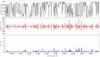 |
Fig. 3. Same as Fig. 2, but for a spectral region around 3140 Å. |
| In the text | |
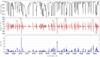 |
Fig. 4. Same as Fig. 2, but for a spectral region around 4080 Å. |
| In the text | |
|
Fig. 5. Relative inversion errors as function of the optical depth for the many-line approaches at 3140 Å (black lines), at 4080 Å (blue lines), and at 6302 Å (green lines) as well as for the double-line approach at 6302 Å (red lines). The errors of the three quantities temperature, magnetic field strength and LOS velocity are shown in the left, middle, and right panel, respectively. |
| In the text | |
|
Fig. 6. Scatter plots (black dots) of the temperature, magnetic field strength, and LOS velocity (from left to right) retrieved from an inversion of synthetic Stokes profiles degraded with realistic photon noise versus the inversion results from noise-free profiles at the optical depth nodes used during the inversion for the spectral region 3128.5 Å−3150 Å that contains 371 relevant spectral lines. The ideal relation for a perfect fit is indicated by the red line. From top to bottom the panels refer to different optical depth nodes (marked in the figures). |
| In the text | |
|
Fig. 7. Same as Fig. 6, but for the spectral region 6300.8 Å−6303.2 Å that only contains the Fe I 6301.5 Å and 6302.5 Å line pair. |
| In the text | |
|
Fig. 8. Excerpts from the Jungfraujoch atlas (solar lines in black color, telluric lines in gray color) and from spatially averaged synthetic spectra (red lines; see main text for details). |
| In the text | |
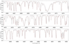 |
Fig. 9. Same as Fig. 8, but for the spectral region around 4080 Å. |
| In the text | |
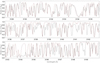 |
Fig. 10. Same as Fig. 8, but for the spectral region around 3140 Å. |
| In the text | |
Current usage metrics show cumulative count of Article Views (full-text article views including HTML views, PDF and ePub downloads, according to the available data) and Abstracts Views on Vision4Press platform.
Data correspond to usage on the plateform after 2015. The current usage metrics is available 48-96 hours after online publication and is updated daily on week days.
Initial download of the metrics may take a while.