© ESO 2018

1 Introduction

Hydrodynamic mechanism of meteoroid ablation as a quasi-continuous spraying of the meteoroid melt was considered in part one of this work (Girin 2017), which is referred to here as Paper I. The mechanism consists in the meteoroid molten substance spraying in the form of fine liquid droplets due to the hydrodynamic “gradient” instability of conjugated (air-melt) boundary layers at the meteoroid body surface. A shallow-angle trajectory and the regime of outstripping melting are assumed in this paper for a compact, almost completely molten meteoroid, the radius of which lies within a certain range. Under these assumptions, behaviour of the meteoroid is equivalent to the one of a liquid drop in a high velocity uniform air flow, so that the gradient instability theory can be directly applied to the process of the liquid particle generation during the meteoroid flight to determine the particle sizes and the instant of their breakaway. As a result, the approximate analytic solution proposed in this study can also be employed to obtain the distribution function of the sprayed molten droplets. However, this problem is complicated by the coupled processes of meteoroid deceleration and ablation, which are mutually influenced.

A meteoroid of spherical shape is considered, which begins to ablate when moving in the continuum regime. In general, the transiency and complexity of the flow geometry around a spherical meteoroid make it necessary to carry out a numerical treatment of the ablation process. The numerical scheme of calculation of the particle breakaway process was elaborated in Paper I, which takes into account the temporal and spatial variations of hydrodynamic parameters along the meteoroid surface. Variations of both (gas–liquid) boundary layer thicknesses were taken into account by applying basic boundary-layer theory relations. The numerical scheme has allowed us to obtain intermediate and final number distributions of the broken away particles by sizes, as well as the meteoroid mass loss law.

Notwithstanding its importance, the melt spraying represents only the initial process of the aerosol formation in a meteor wake. The meteoroid deceleration, mass loss and ensuing processes of the sprayed particles’ acceleration, evaporation, cooling, and solidification results in an involved quantitative description of the overall meteor phenomenon. The processes taking place in meteoric persistent trains set up the physico-chemical conditions in meteor plasmas, which determines afterglow emission spectra and provides very useful data to help understand the composition of the progenitor meteoroids (Madiedo et al. 2014; Drouard et al. 2018). We note that the orders of magnitude of the main parameters of the problem differ significantly one from each other, resulting in difficulties during the calculations. The general problem requires thus simplifications, such as the application of approximate solutions for some elementary processes. Such a solution of the differential equations of meteoroid motion and ablation is obtained in the present work under some additional restrictions. This solution makes it possible to derive an equation for the distribution function of all sprayed particles by sizes, and to solve it in the form of approximate expressions. The distribution function is the key object in many of the atmospheric dust investigations.

2 Equation for broken-away droplet quantification

The general formulation of this problem was described in Paper I, but we refer to some specific points here. It was noted in Paper I that the instability of the meteoroid melt is generated by the gradient flow in the liquid boundary layer, which is imposed tangentially by the co-flowing air. The fastest unstable disturbance is of prime interest in practical applications since it may result in a molten particle breaking-away at the non-linear stage of the disturbance development. Amplification of the fastest disturbances at various area elements of the meteoroid surface is governed by the dependencies of the wavenumber, Δ_f (We_s), and the growth rate factor, $\text{Im}\left[{\Omega }_{\text{f}}(W{e}_{\text{s}})\right]$, on the “surface” Weber number, $W{e}_{\text{s}}={\rho }_{\text{m}}{V}_{\text{s}}^2{\delta }_{\text{m}}/\Sigma$. When applying these dependencies to meteoroid, we found that there exists a critical point on the meteoroid surface, φ_cr (t), where the critical value of the surface Weber number occurs: We_s(φ_cr) = We_s.cr. = 3.08. This critical point divides the meteoroid surface into stable, φ < φ_cr, and unstable, φ > φ_cr, regions. Here φ is the polar angle of the area element on the meteoroid surface (Fig. 3 of Paper I). Assuming a potential flow past a spherical meteoroid, V_a = 1.5(V_∞− w) sin φ, taking the distribution of the air boundary layer thickness along the spherical surface in Ranger’s (1972) form, ${\delta }_{\text{a}}(\phi ,t)=2.2R(t)R{e}_{\infty }^{-0.5}(t)\Psi (\phi )$, and taking into account Eqs. (3) of Paper I, we obtain the following expressions for the boundary layer thickness in the melt and for the gas–liquid mutual velocity at the interface, respectively: $$\begin{array}{lll}\hfill & \hfill & {\delta }_{\text{m}}(\phi ,t)=2.2\frac{{\alpha }^{1/3}}{{\mu }^{2/3}}\frac{R(t)}{R{e}_{\infty }^{0.5}(t)}\Psi (\phi ),\hfill \\ \hfill & \hfill & \text{and}\hfill \\ \hfill & \hfill & V_{\text{s}}(\phi ,t)=\frac{{\alpha }^{1/3}{\mu }^{1/3}}{1+{\alpha }^{1/3}{\mu }^{1/3}}1.5[V_{\infty }-w(t)]\sin \phi .\hfill \end{array}$$(1)

Here $\Psi (\phi )\equiv {[(6\phi -4\sin 2\phi +0.5\sin 4\phi )/{\sin }^5\phi ]}^{0.5}$, α = ρ_a∕ρ_m, μ = μ_a∕μ_m are the air-to-melt density and viscosity ratios, assuming that melt is the Newtonian fluid. Then, the condition We_s (φ) > 3.08 for the gradient instability existence at any area element of meteoroid surface can be rewritten as $$\frac{2.475}{{[1+{(\alpha \mu )}^{1/3}]}^2}\sqrt{\tilde{R}(\tau ){[1-W(\tau )]}^3}{\sin }^2\phi \Psi (\phi )\text{GI}\ge K.$$(2)

Here $\tilde{R}=R/R_0$ and W = w∕V_∞ are the dimensionless current meteoroid radius and velocity deficit due to deceleration, R₀ is the initial meteoroid radius, τ = t∕t_ch, t_ch =2R₀∕α^0.5V_∞ is the timescale, V_∞ is the initial meteoroid velocity, $\text{GI}\equiv W{e}_{\infty }/R{e}_{\infty }^{0.5}$ the gradient instability criterion and K is a constant. The equality in Eq. (2) at K = 3.08 determines the value of φ_cr(τ); at GI > 0.4 and τ = 0 (so that $\tilde{R}=1,W=0$) we have φ_cr < π∕2. This means that the part of the surface adjacent to meteoroid edge, φ_cr < φ < π∕2, is unstable, providing the possibility of melt spraying. The criterion GI is usually large in the meteor phenomenon, GI ≫ GI_cr= 0.4, so that the values φ_cr are small enough: φ_cr ≪ π (e.g. at GI = 43.5 we have φ_cr = 8.8°), such that most of the meteoroid surface generates a mist of liquid particles.

The key parameters of the breakaway process, namely, the disturbance wavelength λ_f , and the characteristic time t_f of its amplitude growth, are both varied along the meteoroid surface and in time. In order to include the breakaway mechanics into the calculating algorithm, we have divided the meteoroid surface on a system of plane elementary areas (more exactly – spherical belts in the axially symmetrical flow) of the width Δ l_i = R(t) Δφ_i (Fig. 4 of Paper I), so that at every time-step the flow parameters may be treated as constant at each ith elementary area. We applied the results of instability analysis to the locally plane flow at each unstable area element, which makes it possible the spraying quantification. This mechanism of instability is governed by the regularities Δ_f (We_s), Im (Ω_f(We_s)), shown in Fig. 5 of Paper I.

Thus, we considered each area element Δl on the unstable part of the meteoroid surface, φ_cr < φ < π∕2, as a source of tiny melt particles (Fig. 4 of Paper I). It is natural to set the size of the breakaway particle as proportional to half-wavelength of the fastest disturbance λ_f, while the period of its breaking-away, t_per, to the time t_f of e-fold growth of the disturbance amplitude at a given ith area element $$r_i=k_{\text{r}}{\lambda }_{\text{f}i},k_{\text{r}}<0.25;t_{\text{per}.i}=k_{\text{t}}{t}_{\text{f}i},k_{\text{t}}\approx 1,$$(3)

where λ_f = 2πδ_m∕Δ_f, t_f = Im⁻¹(Ω_f)δ_m(φ)∕V_s(φ).

When the part of the induction time of the disturbance growth, τ_indi = ∫ dt∕t_per.i, exceeds unity, it is supposed that the separation of the tori of cross-section radius r_i and of number n_{tor i} occurs at that moment from that area element. The quantity of wavelengths, which are confined within ith area element, is equal to n_{tor i}(φ_i) = Δl_i(φ_i)∕λ_{f i}(φ_i). Due to the axial symmetry of the flow past meteoroid, this is the quantity of tori of radius R(t) sinφ_i, which have been broken away from the spherical belt corresponding to Δl_i. Assuming that the liquid torus is quickly breaking into droplets of radius r_i in the high-speed air stream, and taking the overall volume of tori, $\Delta {\upsilon }_i=n_{\text{tor}i}\cdot \Delta {\upsilon }_{\text{tor}i}=\pi k_{\text{r}}^2{\lambda }_{\text{f}i}2\pi R\sin {\phi }_i\cdot \Delta l_i$, divided by the single particle volume, ${\upsilon }_{\text{p}i}=4/3\pi r_i^3$, we obtain the differential equation for the number Δn of newborn particles of radius r(φ, τ): $$\Delta n={\dot{n}}^{\prime }(\phi ,\tau )\Delta \phi \Delta \tau =B_2\sqrt{\tilde{R}(\tau ){[1-W(\tau )]}^5}\frac{{\sin }^2\phi }{{\Psi }^3(\phi )}\Delta \phi \Delta \tau ,$$(4) $$\tilde{r}(\phi ,\tau )=B_{1}T(\tau )\Psi (\phi ),T=\sqrt{\frac{\tilde{R}(\tau )}{1-W(\tau )}},$$(5)

which have been broken away from the area element Δφ in the period Δτ. Here ṅ′(φ, τ) is the rate of particle production, in which the coefficients, given by $$B_1=\frac{4.4\pi k_{\text{r}}}{{\Delta }_{\text{f}}\sqrt{2R{e}_{\infty }}}\frac{{\alpha }^{1/3}}{{\mu }^{2/3}},$$(5’)

and $$B_2=\frac{0.21{\Delta }_{\text{f}}^{\text{2}}\text{Im}({\Omega }_{\text{f}})\sqrt{2R{e}_{\infty }^3}}{\pi k_{\text{r}}{k}_{\text{t}}[1+{(\alpha \mu )}^{1/3}]}\frac{{\mu }^{7/3}}{{\alpha }^{7/6}},$$

can be interpreted as scaling parameters for the particle sizes and number, respectively (Girin 2011a), and the superscript dot stands for the differentiation with respect to τ, while ′– to φ ; $\tilde{r}=r/R_0$.

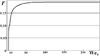Fig. 1 Dimensionless function $F\equiv \text{Im}\left({\Omega }_{\text{f}}\right)/{\Delta }_{\text{f}}$ versus “surface” Weber number $W{e}_{\text{s}}={\rho }_{\text{m}}{V}_{\text{s}}^2{\delta }_{\text{m}}/\Sigma$.

3 Equation of meteoroid mass losses

The mechanism of melt spraying described in Sect. 2 predetermines an alternative form of differential equation of meteoroid ablation, which differs from the classic equation of the general physical theory of meteors (Bronshten 1983). Since the elementary breakaway process occurs in a time period t_per (φ) = k_tt_f(φ) = k_tδ_m(φ)∕V_s(φ)Im(Ω_f), the mass efflux rate can be expressed as $$\begin{array}{l}\frac{\Delta m}{\Delta t}(\phi ,t)=\frac{{\rho }_{\text{m}}\Delta \upsilon (\phi ,t)}{t_{\text{per}}(\phi ,t)}\\ =\text{}\frac{{\rho }_{\text{m}}2{\pi }^2{k}_{\text{r}}^{2}R(t){\lambda }_{\text{f}}(\phi ,\text{}t)\sin \phi \text{}{V}_{\text{s}}(\phi ,t)\text{Im}\left[{\Omega }_{\text{f}}(W{e}_{\text{s}}(\phi ,t))\right]}{k_{\text{t}}{\delta }_{\text{m}}(\phi ,t)}\Delta l(\phi ,t).\end{array}$$(6)

By substituting λ_f = 2πδ_m∕Δ_f in Eq. (6), taking into account Δl = R(t)Δφ, and by integrating over the windward surface from φ = φ_cr(t) to the meteoroid edge φ = π∕2, we obtained the rate of meteoroid mass diminishing $$\begin{array}{l}\frac{\text{d}m}{\text{d}t}\\ =-\frac{4{\pi }^3{k}_{\text{r}}^2}{k_{\text{t}}}{\rho }_{\text{m}}{R}^2(t){\displaystyle {\int }_{{\phi }_{\text{cr}}(t)}^{\pi /2}\frac{V_{\text{s}}(\phi ,t)\text{Im}\left[{\Omega }_{\text{f}}(W{e}_{\text{s}}(\phi ,t))\right]\sin \phi }{{\Delta }_{\text{f}}\left[W{e}_{\text{s}}(\phi ,t)\right]}\text{d}\phi }.\end{array}$$(7)

To simplify the integrand, we note that the function $F(W{e}_{\text{s}})\equiv \text{Im}\left[{\Omega }_{\text{f}}(W{e}_{\text{s}})\right]/{\Delta }_{\text{f}}(W{e}_{\text{s}})$, which in Eq. (7) defines an influence of the fastest disturbance parameters on the mass efflux rate, is almost constant for We_s ≫ We_s.cr. = 3.08 (Fig. 1). It sharply increases in the vicinity of the critical point, so that we can neglect the mass efflux rate at We_s.cr.< We_s < We_s(φ_lt) ≈ 5.0. Besides, this vicinity must be avoided, since the fastest unstable wave length is greater here than the meteoroid diameter, λ_f >2R(t); as well, its characteristic time is greater than the meteoroid breakup time t_spr (see Fig. 5 of Paper I). Therefore, the corresponding unstable disturbances are not able to be accomplished until the overall breakup time. Consequently, the lower limit in Eq. (7) must be replaced by such a value φ_lt >φ_cr, for which k_r λ_f (φ_lt, t) ≾ R(t), k_t t_f (φ_lt) ≾ t_spr. Taking this into account, we were able to adopt F(We_s) = 0.18 as the average constant value within the spraying interval φ_lt(t) < φ ≤π∕2. This assumption is valid for sufficiently large values of the gradient instability criterion: GI ≫GI_cr = 0.4, when φ_cr , φ_lt ≪π, so that the inequality We_s≫ We_s.cr.= 3.08 is satisfied at the majority of the meteoroid surface. Then from Eq. (7) we will have $$\begin{array}{lll}\frac{\text{d}m}{\text{d}t}\hfill & =\hfill & -0.18\frac{6{\pi }^3{k}_{\text{r}}^2{\rho }_{\text{m}}}{k_{\text{t}}[1+{(\alpha \mu )}^{1/3}]}{\left(\alpha \mu \right)}^{1/3}{R}^2(t)[V_{\infty }-w(t)]\hfill \\ \hfill & \hfill & \times {\displaystyle {\int }_{{\phi }_{\text{lt}}(t)}^{\pi /2}{\sin }^2\phi \text{d}\phi },\hfill \end{array}$$(8)

with the help of Eqs. (2). Calculating the integral, we obtain the kinetic equation of meteoroid mass loss: $$\begin{array}{lll}\frac{\text{d}m}{\text{d}t}\hfill & =\hfill & -\frac{1.08{\pi }^3{k}_{\text{r}}^2{\rho }_{\text{m}}}{k_{\text{t}}[1+{(\alpha \mu )}^{1/3}]}{\left(\alpha \mu \right)}^{1/3}{R}^2(t)[V_{\infty }-w(t)]\hfill \\ \hfill & \hfill & \times \left(\frac{\pi }{4}-\frac{{\phi }_{\text{lt}}(t)}{2}+\frac{\sin 2{\phi }_{\text{lt}}(t)}{4}\right).\hfill \end{array}$$(9)

The right-hand side of Eq. (9) expresses the dependence of mass efflux rate on all the main parameters of the process: current meteoroid radius, relative air-meteoroid velocity, physical properties of the media. Surface tension Σ has a stabilizing effect implicitly via the parameter φ_lt: as Σ increases, values of We_s decrease at each area element of the meteoroid surface, so that the critical point ascends to the meteoroid edge, increasing φ_lt and decreasing the spraying surface area as a consequence. Equation (9) may be rewritten in the dimensionless form: $$\frac{\text{d}M}{\text{d}\tau }=-A{\tilde{R}}^2(\tau )[1-W(\tau )]\left(1-\frac{2{\phi }_{\text{lt}}(\tau )}{\pi }+\frac{\sin 2{\phi }_{\text{lt}}(\tau )}{\pi }\right),$$(10)

where $A\equiv \frac{0.405{\pi }^3{k}_{\text{r}}^2}{k_{\text{t}}[1+{(\alpha \mu )}^{1/3}]}{\left(\frac{{\mu }^2}{\alpha }\right)}^{1/6}$ has the sense of the characteristic (initial) rate of the mass efflux, M = m∕m₀.

The integration of Eq. (10) to determine meteoroid ablation law, M(τ), requires the integration of the equation of the meteoroid motion (in order to have W(τ) known) and Eq. (2) (at K = 5.0) – to determine φ_lt(τ). Their intricacy compels us to solve this system equations considering some further simplifying assumptions. We outline the problem solution for the considered case of speedy flows, when GI ≫ GI_cr = 0.4. The latter subsequently results, with the aid of Eq. (2): φ_lt ≪π, sin 2φ_lt ≈ 2φ_lt. Therefore, taking into account the meteoroid spherical shape (i.e. $M={\tilde{R}}^3$) and the identity W ≡α^0.5dX_M∕dτ for the velocity deficit, the integration of Eq. (10) yields: $$\begin{array}{lll}\hfill & \hfill & M(\tau )={\left[1-\frac{A}{3}\left(\tau -{\alpha }^{0.5}{X}_{\text{M}}(\tau )\right)\right]}^3,\hfill \\ \hfill & \hfill & \hfill \\ \hspace{0.17em}\hfill & \hfill & \tilde{R}(\tau )=1-\frac{A}{3}\left(\tau -{\alpha }^{0.5}{X}_{\text{M}}(\tau )\right),\hfill \end{array}$$(11)

where x_M is meteoroid displacement due to the aerodynamic drag, X_M = x_M∕2R₀. Equations (11) indicate clearly the direct dependence of meteoroid ablation law on its deceleration law, X_M = X_M(τ). It is much simpler to obtain first the latter law, which can be done in two ways, empirical and theoretical, as was done for a drop in Girin (2011a).

3.1 Empirical approximation of meteoroid deceleration law

First, we used the experimental data of Reinecke & Waldman (1975), which are valid for a liquid drop in the rarefied air conditions relevant for the reentry flight. These data allow us to express the law of a liquid sphere motion in the form: α ^0.5 X_M(τ) = τ − [1 − exp(−Hτ)]∕H, where H = 2α^0.5 has the sense of the characteristic deceleration due to aerodynamic drag. From here W = 1 − exp(−Hτ). Taking into account the expression for the dimensionless velocity, W = α^0.5 dX_M∕dτ, Eq. (11) yields the meteoroid ablation law: $$M={\tilde{R}}^3={[1-h(1-\exp (-H\tau ))]}^3.$$(12)

The rate ratio h = A∕3H reflects the influence of two competing factors, which govern the meteoroid dynamics: the mass reduction rate (≈ A, see Eq. (10)) due to spraying, and the rate of relaxational reducing of the air-meteoroid relative velocity (≈ H), which in turn diminishes the mass efflux. Due to the extremely small values of the density ratio α in high atmosphere, values of H are small so that the h values are large for meteoroid: h > 10². Equation (12) shows that the meteoroid is completely sprayed at the time instant ${\tau }_{\text{spr}}=H^{-1}\ln \left[h/(h-1)\right]$, which, at h ≫ 1, approximately equals to ${\tau }_{\text{spr}}={[H(h-1)]}^{-1}\approx 3/A$. Comparison of the ablation law (12) with experimental data of Reinecke & Waldman (1975) for atomizing drops indicated their good agreement (Girin 2011a).

3.2 Theoretical law of ablating meteoroid deceleration

The second way to obtain the deceleration law of an ablating meteoroid consists of the direct integration of the differential equation of the meteoroid motion: $${\rho }_{\text{m}}\frac{4}{3}\pi R^3(t)\frac{\text{d}w}{\text{d}t}=\Gamma \pi R^2(t){\rho }_{\text{a}}{\left[V_{\infty }-w(t)\right]}^2,$$(13)

where Γ is the aerodynamic drag coefficient, which for a meteoroid has a value of the order unity (Bronshten 1983). Though the first integral of the system of meteoroid governing equations of the physical theory of meteors can be derived (Pecina & Koten 2009), the integration is usually carried out either with the assumption that meteor deceleration can be neglected, or with the application of numerical methods.

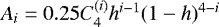
Next, we show that the dynamic equations of the spraying meteoroid theory (Eq. (14)) can be integrated analytically. Modifying Eq. (10) in terms of the meteoroid radius, $\tilde{R}=M^{1/3}$, we obtained for GI ≫ GI_cr the coupled differential equations for the interrelated processes of meteoroid ablation and deceleration with respect to the dimensionless variables $\tilde{R}$ and W: $$\begin{array}{lll}\hfill & \hfill & \frac{\text{d}W}{\text{d}\tau }=C\frac{{(1-W)}^2}{\tilde{R}};\hfill \\ \hfill & \hfill & \frac{\text{d}{M}^{1/3}}{\text{d}\tau }=\frac{\text{d}\tilde{R}}{\text{d}\tau }=-\frac{A}{3}(1-W),\hfill \end{array}$$

with the initial conditions $\tilde{R}(0)=1$, W(0) = 0; here C = 1.5α^0.5Γ has the sense of the characteristic (initial) meteoroid deceleration. By eliminating the velocity term from Eqs. (14) and (15) we obtained a second-order equation with respect to the meteoroid radius: $$\tilde{R}\frac{{\text{d}}^2\tilde{R}}{\text{d}{\tau }^2}={\left(\frac{\text{d}\tilde{R}}{\text{d}\tau }\right)}^2.$$(15)

Here, we have the meteoroid dynamic criterion in the form h = A∕3C, which assumes large values since C is small. At h > 1 the integration of Eq. (15) with initial conditions $\tilde{R}(0)=1,\dot{\tilde{R}}(0)=-A/3$ (the latter follows from Eq. (15)) leads to a solution expressed in terms of power functions. Eventually, we obtain the ablationand deceleration laws in the form $$\begin{array}{lll}\hfill & \hfill & \tilde{R}=\left[1-C(h-1)\tau \right]{}^{h/(h-1)},\hfill \\ \hfill & \hfill & W=1-\left[1-C(h-1)\tau \right]{}^{1/(h-1)}.\hfill \end{array}$$

The laws (Eq. (15)) are applicable until the moment τ_spr , when the meteoroid is totally sprayed, R = 0. From Eq. (15) we have: ${\tau }_{\text{spr}}={[(h-1)C]}^{-1}$ ( ≈ 3∕A for h ≫ 1); the same as in Sect. 3.1. The expression for $\tilde{R}$ in Eq. (15) shows that, due to large h values, the dependence of the ablating meteoroid radius on time is close to linear in the count-down timescale, τ_spr −τ. This conclusion agrees well with both, the empirically approximated dependence (Eq. (12)), taking into account small values of H, and the results from our numerical model (see Paper I). Equation (15) shows that the spraying proceeds at almost unchangeable air–meteoroid relative velocity. The latter is due to the fact that the characteristic time of meteoroid spraying, 3∕A, is several orders smaller than the one of deceleration, C⁻¹, and the rate ratio of these processes, h, is large. However, the meteoroid decelerates suddenly to zero relative velocity at the moment when the meteoroid is completely sprayed, $\tilde{R}=0$. The meteoroid deceleration tends to infinity at that moment; this is caused by the meteoroid radius vanishing, which raises the aerodynamic drag force, as shown by Eq. (14) at $\tilde{R}\to 0$. This explains the sharp-ending deceleration of meteoroid, and agrees with previous observations (Bronshten 1983; Simonenko 1974).

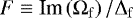
From Eqs. (15) and (15) we can conclude that the rate ratio h is a dynamic similarity criterion, which determines the form of the main dynamic laws of meteoroid behaviour. Moreover, its value determines the dominant process in the ablation–deceleration competition, which is illustrated by the analysis of the dynamic (R, U)-diagrams discussed below.

The obtained laws (Eq. (15)) show that the overall meteoroid behaviour is regulated by two characteristic parameters: its deceleration C and the mass loss rate A. Their values reflect two aspects of the aerodynamic action on meteoroid surface: the integral normal force together with viscous friction force decelerate the meteoroid, while the high-speed tangential slipping along the meteoroid surface causes its instability, which pulls out liquid particles from the melt. The meteoroid reaction is reflected in the character changing of two main dependant parameters - its relative velocity U = 1 − W and its degree of fragmentation, which can be measured by the current dimensionless radius, $\tilde{R}=R/R_0$. Thus, the meteoroid reaction can be represented by its portrayal in $(\tilde{R},U)$-plane, which, depending on A and C, forms a set of ballistic $(\tilde{R},U)$-diagrams showing a variety of ablating meteoroid behaviours in the atmosphere. However, in view of Eq. (15) the meteoroid $(\tilde{R},U)$-diagrams are all expressed by the one-parameter set of curves: $U={\tilde{R}}^{1/h}$, with the unique parameter h. Examples are shown in Fig. 2, calculated for the meteoroids in the present paper.

The meteoroid flight is exceptionally characterized by small C values, while A has the order of unity, which yields large h = A∕3C. Since the values of A and C are determined mostly by the physical properties of meteoroid substance, for every pure substance there exists a single regime of an ablating meteoroid behaviour, which is independent of the initial meteoroid velocity and size. As the curves in Fig. 2 show, the majority of the ablating meteoroid flight is performed at conditions of an intense air motion past the meteoroid, when the relative air-meteoroid velocity remains close to the initial value U₀ = 1. Thus, the diagrams show that due to large h values the meteoroid is always held in regime of dynamic ablation, when the airflow impact is shifted towards the spraying action, so that the majority of the airstream energy is spent to increase the melt instability, while the minor part is used for meteoroid deceleration. In this connection, one can see in Fig. 2 that iron meteoroid spraying is more efficient than that of stone. For instance, at the same 1% degree of meteoroid deceleration (or U = 0.99), the degree of the stony meteoroid fragmentation is ≈30% less than that of the iron meteoroid, independently of the initial meteoroid velocity. The effect is expressed also by the shorter amount of time needed for full meteoroid fragmentation and finer pulverization of the iron meteoroid. The reason for this effect lies obviously in the media physical properties (namely, the 30-fold viscosity difference leads to a difference of approximately 5.3 in h), as seen in Paper I. When the viscosity of the molten substance is even greater than the stony one, the $(\tilde{R},U)$-diagram descends lower, showing the possibility of incomplete spraying of completely molten meteoroids. Thus, the parameter h plays a role of a similarity criterion for the dynamic behaviour of meteoroid. Under the adopted assumptions for the considered class of meteoroids, we can conclude that the meteoroids made of the same substance have a similar behaviour during their flight, irrespective of their initial velocities and sizes.

Fig. 2 Dynamic radius-velocity ($\tilde{R},U$)-diagrams for the stone, h = 125, (curve 1 – V∞ = 60 km sec−1) and iron, h = 662, (crimson + light-green curve 2 – V∞ = 25 km sec−1, light-green curve 3 – V∞ = 60 km sec−1) meteoroids.

4 Sprayed-droplet distribution function

The melt-spraying model allows quantifying the dispersion process in detail. Integrating Eq. (4) for the newborn particle number throughout the domain of spraying in the (φ , τ)-plane, we would find the total number of the broken-away particles. However, the most important parameter used in the description of the meteoroid ablation is the transient distribution function of the broken-away particles by sizes, $f_{\text{n}}(\tilde{r},\tau )=\Delta n(\tilde{r},\tau )/\Delta \tilde{r}$, which is needed for the quantitative description of the aerosol formation in the meteor wake and its further evolution. Such distributions for ablating meteoroids are unknown to us, neither theoretical, nor empirical. Obtained regularities (Eqs. (4), (5), (12), and (15)) allow us to know the approximate distribution function of newborn particles by sizes.

In order to obtain the differential distribution function $f_{\text{n}}(\tilde{r},\tau )$, we need to integrate the equation for particle production rate ṅ′(φ, τ) (Eq. (4)) along each line $\tilde{r}(\phi ,\tau )=L$ (referred to in the sense of Eq. (5)) over a strip of width $\Delta \tilde{r}=Q$, where L and Q are constants. Hence, we must first build the spraying domain in the plane of events (φ , τ), which is shown in Fig. 3 together with the calculated set of lines $\tilde{r}(\phi ,\tau )=L={\tilde{r}}_{\text{fix}}$. The top and left regions of the spraying domain are bounded by the curve φ =φ_lt(τ), while the bottom region by the initial moment τ = 0. The meteoroid edge position, φ_rt = π∕2, defines the right boundary of the domain. The spraying domain can be divided conditionally into the two parts, I and II, by the line $\tilde{r}={\tilde{r}}_{\text{fix}.\text{lt}.}=\tilde{r}[{\phi }_{\text{lt}}(0),0]$, which leaves the point φ_{lt 0} = φ_lt(0). These lines, which lie at the bottom section of region (sub-domain I), start at τ = 0 and end at φ =π∕2; the lines above, in sub-domain II, start at the left-boundary curve, φ = φ_lt(τ), and end at φ = π∕2. It follows then from Eq. 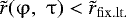(5) that $\tilde{r}(\phi ,\tau )>{\tilde{r}}_{\text{fix}.\text{lt}.}$ in sub-domain I and $\tilde{r}(\phi ,\tau )<{\tilde{r}}_{\text{fix}.\text{lt}.}$ in sub-domain II, since $T(\tau )={[\tilde{R}(\tau )/(1-W(\tau ))]}^{0.5}$ is the decreasing function (for h > 1) and Ψ(φ) is the increasing one.

Spraying starts at τ = 0 from the area elements Δφ within the interval φ_{lt 0} ≤φ ≤π∕2, which represents the unstable part of the meteoroid surface. As Fig. 3 shows, at the very beginning, the breakaway particle sizes lie within the basic range, ${\tilde{r}}_{\text{fix}.\text{lt}.}\le \tilde{r}\le {\tilde{r}}_{\text{fix}.\text{rt}.}$, which corresponds to the endpoints of the initial segment φ_{lt 0} ≤φ ≤π∕2. Since T(0) = 1, here we have ${\tilde{r}}_{\text{fix}.\text{lt}.}=B_1\Psi ({\phi }_{\text{lt}0})=\sqrt{3.2}{B}_1$ and ${\tilde{r}}_{\text{fix}.\text{rt}.}=B_1\Psi (\pi /2)=\sqrt{3\pi }{B}_1$. The spraying process then goes gradually into sub-domain II, where $\tilde{r}<{\tilde{r}}_{\text{fix}.\text{lt}.}$, therefore the particle coarse fraction is generated always at the beginning, while the fine fraction – at the end of the ablation process. For this reason, the newborn particle sizes diminish in time, as shown in calculations in Paper I, and clearly seen in the supplemental material of Paper I (video files Movie 1 and Movie 2). The instant when the left boundary of the spraying domain (black line 2) intersects the right boundary is the moment of the meteoroid spraying termination, τ = τ_spr.

In order to determine $f_{\text{n}}(\tilde{r},\tau )$, we need to eliminate Ψ(φ) from Eq. (4) with the help of Eq. (5) and substitute $\Delta \tau =\Delta \tilde{r}/\left[B_1\dot{T}(\tau )\Psi (\phi )\right]$, which represents the strip with $\Delta \tilde{r}$ width in τ -direction. Then, integrating Eq. (4) along the line $\tilde{r}(\phi ,\tau )={\tilde{r}}_{\text{fix}}$ from the lower limit [${\phi }_{*}=\phi (0;{\tilde{r}}_{\text{fix}})$ in sub-domain I, and 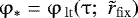${\phi }_{*}={\phi }_{\text{lt}}(\tau ;{\tilde{r}}_{\text{fix}})$ in sub-domain II] to the upper limit, φ^* = π∕2, we obtain equation for the distribution function $f_{\text{n}}({\tilde{r}}_{\text{fix}},\tau )$: $$\begin{array}{lll}\Delta n\hfill & =\hfill & f_{\text{n}}({\tilde{r}}_{\text{fix}},\tau )\Delta \tilde{r}=\frac{2B_1^3{B}_2}{(h-1)H{\tilde{r}}_{\text{fix}}^4}\hfill \\ \hfill & \hfill & \times {\displaystyle {\int }_{{\phi }_{*}}^{\pi /2}{\tilde{R}}^3[\tau (\phi )][1-W(\tau (\phi ))]{\sin }^2\phi \text{d}\phi }\Delta \tilde{r},\hfill \end{array}$$(17)

in which the dependence τ(φ) ought to be determined from the Eq. (5) for every fixed ${\tilde{r}}_{\text{fix}}$. Equation (17) clearly shows that both the meteoroid ablation and deceleration laws influence the distribution function.

The evaluation of the curvilinear integral in (17) is a knotty problem in view of kind of the dependence $\tau (\phi ;{\tilde{r}}_{\text{fix}})$ (see Eq. (5) at $\tilde{r}={\tilde{r}}_{\text{fix}}$, and Eqs. (12) and (15)) so that approximation methods can be useful. We can point out two of the possible ways based on the empirical and analytical approaches of Sect. 2.

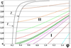Fig. 3 Set of lines $\tilde{r}(\phi ,\tau )=L$ (coloured) on the plane of events for the iron meteoroid spraying; GI = 16.8, τspr = 4.06. Black line 1 – left boundary φ = φcr(τ) of unstable part of meteoroid surface; black line 2 – left boundary φ = φlt(τ) of spraying domain. Dashed green band shows the strip of integration, $\Delta \tilde{r}=Q$, for ${\tilde{r}}_{\text{fix}}=\tilde{r}({\phi }_{\text{lt0}})$.

4.1 Distribution function for the empirical approximation

Using the expressions for the empirical approximation of the meteoroid deceleration law (Eq. (12)), the equation of line $\tilde{r}={\tilde{r}}_{\text{fix}}$ in the (φ , τ)-plane can be implicitly written as follows: $$\tau (\phi ;{\tilde{r}}_{\text{fix}})=H^{-1}\ln \left[\frac{h-{[{\tilde{r}}_{\text{fix}}/B_1\Psi (\phi )]}^2}{h-1}\right],$$(18)

and Eq. (17) for the distribution function becomes: $$\begin{array}{l}\Delta n=f_n\Delta \tilde{r}=\frac{2B_1^3{B}_2}{\left(h-1\right)}H{\tilde{r}}_{\text{fix}}^4\\ \times \underset{{\varphi }_{*}}{\overset{\pi /2}{\int }}{\left[1-h+h\exp \left(-H\tau \right)\right]}^3\exp \left(-H\tau \right){\sin }^2\varphi \text{d}\varphi \Delta \tilde{r}.\end{array}$$(19)

We see from Fig. 3 that in the case h ≫ 1 the lines $\tilde{r}(\phi ,\tau )={\tilde{r}}_{\text{fix}}$ are only slightly curved so that the path of integration in Eq. (19) can be approximated by the straight line τ − τ_* = (φ −φ_*)∕a_ef with some effective slope $a_{\text{ef}}({\tilde{r}}_{\text{fix}},h)$. Then, using the tabular integral ${\displaystyle \int e^{q\phi }}{\sin }^2\phi \text{d}\phi =e^{q\phi }/2q-e^{q\phi }\left(0.5q\cos 2\phi +\sin 2\phi \right)/(q^2+4)$ (Gradshtein & Ryzhyk 1980) and the laws (12), we obtain, after integrating Eq. (19): $$\begin{array}{ll}\Delta n({\tilde{r}}_{\text{fix}})\hfill & =f_{\text{n}}({\tilde{r}}_{\text{fix}})\Delta \tilde{r}\hfill \\ \hspace{0.17em}\hfill & =\frac{B_1^3{B}_2}{(h-1){\tilde{r}}_{\text{fix}}^4}\frac{a_{\text{ef}}(\tilde{r})}{H^2}{\displaystyle \sum _{i=1}^4{A}_i}\left[{\Phi }_{i*}({\tilde{r}}_{\text{fix}})-{\Phi }_i^{*}({\tilde{r}}_{\text{fix}})\right]\Delta \tilde{r},\hfill \end{array}$$(20)

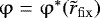where ${\Phi }_i({\tilde{r}}_{\text{fix}})=D^i({\tilde{r}}_{\text{fix}})\left[{\sin }^2\phi ({\tilde{r}}_{\text{fix}})+{\sin }^2\left[\phi ({\tilde{r}}_{\text{fix}})+{\theta }_i({\tilde{r}}_{\text{fix}})\right]\right]$ must be calculated at the lower, $\phi ={\phi }_{*}({\tilde{r}}_{\text{fix}})$, and upper, $\phi ={\phi }^{*}({\tilde{r}}_{\text{fix}})$, limits of integration, correspondingly; $D({\tilde{r}}_{\text{fix}})=(h-1)/\left[h-{\left[{\tilde{r}}_{\text{fix}}/(B_1\Psi (\phi ))\right]}^2\right]$; $A_i=0.25C_4^{(i)}{h}^{i-1}{(1-h)}^{4-i}$; $C_4^{(i)}$ are the binomial coefficients, ${\theta }_i=\text{arc}\sin {\left[1+{(iH/2a_{\text{ef}})}^2\right]}^{-0.5}$ at h > 1. Values of ${\phi }_{*}({\tilde{r}}_{\text{fix}})$ in sub-domain I are to be found from Eq. (18) at τ = 0. In sub-domain II the system of Eq. (18) of the line $\tilde{r}(\phi ,\tau )={\tilde{r}}_{\text{fix}}$ coupled with the equation of the left boundary φ_lt(τ) of the spraying domain (Eq. (2) at K = 5.0) must be solved. In order to simplify the calculations, the expression Eq. (20) is simplified at the upper limit, φ ^* = π∕2, where sin φ^* = 1, cos φ^* = 0 and at the lower limit in the initial segment, where τ_* = 0, D = 1.

Analysis of the behaviour of lines $\tilde{r}(\phi ,\tau )={\tilde{r}}_{\text{fix}}$ allows us to find the expression for a_ef, which is valid for a wide range of h values (Girin 2011b). The effective slope a_ef must be fitted accounting for the influence of both, the initial value 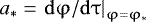$a_{*}={\text{d}\phi /\text{d}\tau |}_{\phi ={\phi }_{*}}$ and the mean value a_{m.v .} = (φ^*−φ_*)∕(τ^*−τ_*). Eventually, the following expressions for a_ef are obtained in sub-domains I and II: $$\begin{array}{lll}\hfill & \hfill & a_{\text{ef}I}=\frac{\left(h+2.1/h^{0.5}\right)a_{\text{m}.\text{v}.}{a}_{*}}{h{a}_{*}+a_{\text{m}.\text{v}.}{h}^{-2}+(a_{\text{m}.\text{v}.}+a_{*})/h^{0.5}},\hfill \\ \hfill & \hfill & a_{\text{ef}II}=\frac{\left(1.133h+0.867/h^2\right)a_{\text{m}.\text{v}.}}{h}.\hfill \end{array}$$(21)

Equations (20) and (21) permit us to obtain not only the final distribution, but also the expression for any current distribution, which has formed until the arbitrary moment τ_c < τ_spr. For this purpose, it is sufficient to determine the values ${\phi }^{*}({\tilde{r}}_{\text{fix}},{\tau }_{\text{c}})$, $a_{\text{ef}}({\tilde{r}}_{\text{fix}},{\tau }_{\text{c}})$, ${\theta }_i({\tilde{r}}_{\text{fix}},{\tau }_{\text{c}})$, $D({\tilde{r}}_{\text{fix}},{\tau }_{\text{c}})$ at τ = τ_c $\forall {\tilde{r}}_{\text{fix}}$, which can be done by the same formulae.

4.2 Distribution function for the theoretical laws of an ablating meteoroid

The distribution function (Eq. (20)) was derived based on the empirical law of the meteoroid motion (Eq. (12)), which represented quantitatively well the physical phenomenon observed. To eliminate influence of the arbitrary form of the empirical law, the procedure of obtaining $f_{\text{n}}(\tilde{r})$ is undertaken in a similar way, but it is grounded now on theoretical laws (Eq. (15)). For the expressions Eq. (15), the equation of line $\tilde{r}={\tilde{r}}_{\text{fix}}$ in the (φ , τ)-plane can be implicitly expressed as follows: $$\tau (\phi ;{\tilde{r}}_{\text{fix}})=\frac{1}{(h-1)C}\left[1-{\left(\frac{{\tilde{r}}_{\text{fix}}}{B_1\Psi (\phi )}\right)}^2\right].$$(22)

In a similar way, with the help of Eqs. (5) and (15), we obtained the equation for the differential distribution function: $$\Delta n=f_{\text{n}}({\tilde{r}}_{\text{fix}},\tau )\Delta \tilde{r}$$ $$=\frac{2B_1^3{B}_2}{C(h-1){\tilde{r}}_{\text{fix}}^4}{\displaystyle {\int }_{{\phi }_{*}}^{{\phi }^{*}}{\left[1-C(h-1)\tau (\phi )\right]}^{\eta }}{\sin }^2\phi \text{d}\phi \Delta \tilde{r},$$(23)

in which η = 3h∕(h − 1). The variable of integration can be transformed from φ to 2φ, so that we can use the tabular integral ∫ P_η(φ)cos2φ dφ = $\frac{\sin 2\phi }{2}{\displaystyle \sum _{k\text{=0}}^{\text{E}(\eta \text{/2})}{(-1)}^k\frac{P_{\eta }^{(2k)}(\phi )}{2^{2k}}+}\frac{\cos 2\phi }{2}{\displaystyle \sum _{k\text{=1}}^{\text{E}((\eta +1)\text{/2})}{(-1)}^{k-1}\frac{P_{\eta }^{(2k-1)}(\phi )}{2^{2k-1}}}\equiv F_{\eta }(\phi )$, which is valid for integer η (see Gradshtein & Ryzhyk 1980). Then, integrating along the straight τ −τ_* = (φ −φ_*)∕a_ef, we obtained the distribution function in the polynomial form $$f_{\text{n}}({\tilde{r}}_{\text{fix}})=\frac{3h{B}_1^3{B}_2}{(h-1)A{\tilde{r}}_{\text{fix}}^4}{\left[\frac{1}{c(\eta +1)}{P}_{\eta +1}(\phi )-F_{\eta }(\phi )\right]}_{{\phi }_{*}}^{{\phi }^{*}}.$$(24)

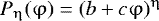Here $P_{\eta }(\phi )={(b+c\phi )}^{\eta }$ is a polynomial, $P_{\eta }^{(k)}$ – its kth derivative, $b=1-(h-1)C\left({\tau }_{*}-{\phi }_{*}/a_{\text{ef}}\right)$, c = −(h − 1)C∕a_ef, and E( x) is the entire part of x. The series of discrete values of h: 1 < h = η∕(η − 3) ≤ 4 corresponds to natural η > 3. For integers η < 0 we obtained a series of h values, which belong to the interval 0.25 ≤ h < 1 of incomplete regimes of drop fragmentation (Girin 2011b); in this case f_n is expressed by the integral sine and cosine functions, Si(φ), Ci (φ).

The aforementioned set of η values covers densely enough all the practically important range of h. The real meteor conditions correspond to h ≫ 1, which are consonant with η = 3, η = 4, being closer to the former value. In order to simplify the calculations, (Eq. (24)) is simplified at the upper limit, φ ^* = π∕2, where sin 2φ^* = 0, cos 2φ^* = −1 and at the lower limit for the basic range, where τ_* = 0, P_η(φ₀) = 1. We give here the final formulae for the calculation of the integral in Eq. (23) for the case η = 3. Namely, in sub-domain I: $$\begin{array}{l}{\displaystyle {\int }_{{\phi }_{*}}^{{\phi }^{*}}{(b+c\phi )}^3{\sin }^2\phi \text{d}\phi }=\frac{1}{8c}\left(A_1^4-1\right)+\frac{3c}{8}\left(A_1^2-\frac{c^2}{2}\right)\\ +\frac{1}{4}\left(1-\frac{3}{2}{c}^2\right)\sin 2{\phi }_0+\frac{3c}{8}\left(1-\frac{c^2}{2}\right)\cos 2{\phi }_0,\end{array}$$(25)

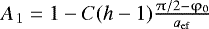where $A_1=1-C(h-1)\frac{\pi /2-{\phi }_0}{a_{\text{ef}}}$. In sub-domain II: 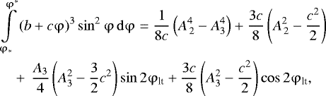$$\begin{array}{l}{\displaystyle {\int }_{{\phi }_{*}}^{{\phi }^{*}}{(b+c\phi )}^3{\sin }^2\phi \text{d}\phi }=\frac{1}{8c}\left(A_2^4-A_3^4\right)+\frac{3c}{8}\left(A_2^2-\frac{c^2}{2}\right)\\ +\frac{A_3}{4}\left(A_3^2-\frac{3}{2}{c}^2\right)\sin 2{\phi }_{\text{lt}}+\frac{3c}{8}\left(A_3^2-\frac{c^2}{2}\right)\cos 2{\phi }_{\text{lt}},\end{array}$$(26)

where A₂ = 1 + c(a_efτ_lt + π∕2 −φ_lt), A₃ = 1 + ca_efτ_lt. In this case, Eq. (22) instead of Eq. (18) should be used to calculate the values φ_* , φ^*. The requirements of the effective slope evaluation remain the same and lead to the expressions $$a_{\text{ef}I}=\frac{\left(1.05h+4.\text{18}{h}^{-0.5}\right)a_{\text{m}.\text{v}.}{a}_{*}}{h{a}_{*}+a_{\text{m}.\text{v}.}{h}^{-2}+(a_{\text{m}.\text{v}.}+a_{*})h^{-0.5}},$$ $$a_{\text{ef}II}=\frac{\left(1.137h+0.867\right)a_{\text{m}.\text{v}.}{a}_{*}}{h{a}_{*}+a_{\text{m}.\text{v}.}}.$$(27)

Equations (25)–(27) permit to obtain not only the final distribution, but additionally the current distribution, which is formed to any arbitrary moment τ_c < τ_spr. For this purpose, it is sufficient to determine the values ${\phi }^{*}({\tilde{r}}_{\text{fix}},{\tau }_{\text{c}})$, $a_{\text{ef}}({\tilde{r}}_{\text{fix}},{\tau }_{\text{c}})$, ${\theta }_i({\tilde{r}}_{\text{fix}},{\tau }_{\text{c}})$, $D({\tilde{r}}_{\text{fix}},{\tau }_{\text{c}})$ at the instant τ = τ_c $\forall {\tilde{r}}_{\text{fix}}$, which can be done by the same formulae.

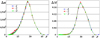Fig. 4 Broken-away particle number, Δn, and mass, ΔM, distributions; r in μm. Iron meteoroid, V∞ = 60 km s−1, GI = 13, φlt 0 = 17.4°, h = 662, A = 1.10, rfix (φlt 0) = 26.4 μm. Curve 1 – calculated by Eqs. (20) and (21); curve 2 – by Eq. (25)-(27); curve 3 – by direct numerical integration of Eqs. (7) and (8) of Paper I, correspondingly.

5 Results and discussion

The broken-away droplet distributions calculated with the use of the empirical and theoretical meteoroid deceleration laws (Eqs. (20), (21), and (25)–(27), correspondingly) are given in Figs. 4–6 (curves 1, 2, correspondingly) for three different meteoroids, whose full input data are given in Paper I. Due to the lack of experimental data on particle size distribution in a meteor wake, the results of the present calculations are compared with those obtained by direct numerical integration of Eqs. (7) and (8) of Paper I (curves 3). One can see that the approximate formulae obtained in the present paper agree well for the high velocity meteoroids, when the assumption GI ≫ GI_cr = 0.4 is fulfilled.

However, it ought to be noted that application of the Eq. (20) of the empirical law at large values of h leads to numerical oscillations in the fine fraction and requires methods of higher accuracy. Nevertheless, this deviation is small when considering the mass distribution, as shown in Figs. 4–6. In contrast, Eqs. (25)–(27) based on theoretical approach, work uniformly well.

Figure 6 shows that the approximate solution is not valid if the main assumption of the presented approach, GI ≫ GI_cr, is not satisfied. The agreement gradually becomes worse because of the influence of the “hump” in Δ_f (We_s) dependence shown in Fig. 3 of Paper I, which was not taken into account in the present approximate approach. As it was noted in Paper I, this effect gives two-humped particle distribution, which cannot be reproduced by the approximate method, as shown in the example in Fig. 6 for GI = 3.55. Hereunder, the condition GI ≫ GI_cr establishes the limits of the elaborated approximate model application.

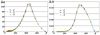Fig. 5 Broken-away particle number, Δn, and mass, ΔM, distributions; r in μm. Stony meteoroid, V∞ = 60 km s−1, GI = 43.5, φlt 0 = 8.8°, h = 125, A = 0.31, rfix (φlt 0) = 330 μm. Curve 1 – calculated by Eqs. (20) and (21); curve 2 – by Eqs. (25)–(27); curve 3 – by direct numerical integration of Eqs. (7) and (8) of Paper I, correspondingly.

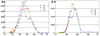Fig. 6 Broken-away particle number, Δn, and mass, ΔM, distributions; r in μm. Iron meteoroid, V∞ = 25 km s−1, GI = 3.55, φlt 0 = 31.8°, h = 662, A = 1.10, rfix (φlt 0) = 42.5 μm. Curve 1 – calculated by Eqs. (20) and (21); curve 2 – by Eqs. (25)–(27); curve 3 – by direct numerical integration of Eqs. (7) and (8) of Paper I, correspondingly.

6 Conclusions

The basic approximate relationships of the ablating meteoroid dynamics for the case of a shallow angle of the meteor trajectory are derived through the application of the theory of meteoroid melt spraying due to the mechanism of gradient instability. Three main processes, meteoroid mass loss, meteoroid deceleration and the melt droplet breakaway kinetics, are interrelated. Therefore, finding out the number distribution of the breakaway particles by sizes requires solving this trinal problem, for which approximate laws are obtained analytically in the present paper under some simplifying assumptions. The solution obtained here provides the intermediate and final number distributions in the form of the approximate relationships (Eqs. (20), (21), or (25)–(27)). Simultaneously, the meteoroid mass loss law is obtained together with the motion law of an ablating meteoroid by the integration of the governing differential equations. The verification was done by comparing the obtained approximate formulae with the solution derived through the accurate integration of the governing equations by the numerical scheme listed in Paper I and showed their agreement. The limits of the approximate solution applicability are established.

As an advantage, the theoretical approach presented herein allows analysing the ablating meteoroid dynamics. The built (R, U) diagrams show that the meteoroid is always held in the regime of dynamic ablation, when the aerodynamic effect is shifted towards the spraying action, so that the majority of the airstream energy is spent to support the hydrodynamic instability of the melt, while the minor part, on the meteoroid deceleration. Thus, the meteoroid ablation proceeds at almost utmost, initial value of the relative airstream velocity. The sharp decrease of the relative velocity at the end of the meteoroid trajectory is only due to the meteoroid radius vanishing, which rises the meteoroid deceleration to infinity. Radius of the ablating meteoroid decreases near-linearly with time.

The h-criterion, which governs the meteoroid ablation-to-deceleration rate balance, is revealed, which depends only on the air-melt density and viscosity ratios and is independent of the meteoroid velocity and size. The h-criterion values of an iron meteoroid are larger than those of a stony due to the smaller melt viscosity. Therefore, the melt spraying proceeds more efficiently for an iron than for a stony meteoroid. We remind the reader that the obtained results are valid within the frames of the main assumptions, namely, a shallow-angle meteor trajectory, the range of sizes of the completely molten meteoroids, large value of the gradient instability criterion, GI ≫GI_cr, and meteoroid spherical shape.

The obtained relationships are necessary as the initial data for the solution of some practical problems of the meteor phenomena. Either full numerical scheme listed in Paper I, or the approximate relations obtained here, can be applied to problems of aerosol formation in meteor wakes. The presented theory of the molten meteoroid spraying can serve as the basis for elaborating future mathematical models for the aerodynamics of accelerating and evaporating mist of the broken-away melt particles, which constitutes an aerosol structure of a meteor wake, permitting to calculate the meteor light curve and to compare it with the observed one. Similar wake models were elaborated for the case of an atomizing drop in a high velocity gas flow in one-dimensional (Girin 2012) and two-dimensional approximations (Girin 2014). Besides, the obtained results help us to understand the underlying dynamics of an ablating meteoroid in its connection with aerosol formation in a meteor wake, being known that they are all interrelated. The proposed theory can also be extended to a general case of a meteoroid entering atmosphere at an arbitrary entry angle.

Appendix A Nomenclature

B1, B2	scaling parameters
$\text{GI}\equiv W{e}_{\infty }R{e}_{\infty }^{-0.5}$	gradient instability criterion
h = A∕3C	rate ratio of ablation-to-
	deceleration processes
Im−1(ω)	growth rate factor
kr, kt	coefficients in Eq. (3)
K, L, Q	constants
m	meteoroid mass
M ≡ m∕m0
R	current meteoroid radius
$\tilde{R}\equiv R/R_0$
r	breakaway droplet radius
$\tilde{r}\equiv r/R_0$
Re∞≡ρ∞2R0V∞∕μ∞	Reynolds number for meteoroid
t	elapsed time
tch ≡ 2R0∕α0.5V∞	characteristic timescale
V	velocity
w	meteoroid velocity deficit due to
	aerodynamic drag
W ≡ w∕V∞
$W{e}_{\infty }\equiv {\rho }_{\infty }{V}_{\infty }^{2}2R_0/\Sigma$	Weber number for meteoroid
$W{e}_{\text{s}}\equiv {\rho }_{\text{m}}{V}_{\text{s}}^2{\delta }_{\text{m}}/\Sigma$	surface Weber number
xM	meteoroid displacement due to
	aerodynamic drag
XM = xM∕2R0
z	meteor altitude.

Greek symbols:

Indices:

References

All Figures

	Fig. 1 Dimensionless function $F\equiv \text{Im}\left({\Omega }_{\text{f}}\right)/{\Delta }_{\text{f}}$ versus “surface” Weber number $W{e}_{\text{s}}={\rho }_{\text{m}}{V}_{\text{s}}^2{\delta }_{\text{m}}/\Sigma$.
In the text

	Fig. 2 Dynamic radius-velocity ($\tilde{R},U$)-diagrams for the stone, h = 125, (curve 1 – V∞ = 60 km sec−1) and iron, h = 662, (crimson + light-green curve 2 – V∞ = 25 km sec−1, light-green curve 3 – V∞ = 60 km sec−1) meteoroids.
In the text

Fig. 3 Set of lines $\tilde{r}(\phi ,\tau )=L$ (coloured) on the plane of events for the iron meteoroid spraying; GI = 16.8, τspr = 4.06. Black line 1 – left boundary φ = φcr(τ) of unstable part of meteoroid surface; black line 2 – left boundary φ = φlt(τ) of spraying domain. Dashed green band shows the strip of integration, $\Delta \tilde{r}=Q$, for ${\tilde{r}}_{\text{fix}}=\tilde{r}({\phi }_{\text{lt0}})$.

In the text

	Fig. 4 Broken-away particle number, Δn, and mass, ΔM, distributions; r in μm. Iron meteoroid, V∞ = 60 km s−1, GI = 13, φlt 0 = 17.4°, h = 662, A = 1.10, rfix (φlt 0) = 26.4 μm. Curve 1 – calculated by Eqs. (20) and (21); curve 2 – by Eq. (25)-(27); curve 3 – by direct numerical integration of Eqs. (7) and (8) of Paper I, correspondingly.
In the text

	Fig. 5 Broken-away particle number, Δn, and mass, ΔM, distributions; r in μm. Stony meteoroid, V∞ = 60 km s−1, GI = 43.5, φlt 0 = 8.8°, h = 125, A = 0.31, rfix (φlt 0) = 330 μm. Curve 1 – calculated by Eqs. (20) and (21); curve 2 – by Eqs. (25)–(27); curve 3 – by direct numerical integration of Eqs. (7) and (8) of Paper I, correspondingly.
In the text

	Fig. 6 Broken-away particle number, Δn, and mass, ΔM, distributions; r in μm. Iron meteoroid, V∞ = 25 km s−1, GI = 3.55, φlt 0 = 31.8°, h = 662, A = 1.10, rfix (φlt 0) = 42.5 μm. Curve 1 – calculated by Eqs. (20) and (21); curve 2 – by Eqs. (25)–(27); curve 3 – by direct numerical integration of Eqs. (7) and (8) of Paper I, correspondingly.
In the text

References

- Bronshten, V. A. 1983, Physics of Meteoritic Phenomena (Dordrecht: Reidel) [Google Scholar]
- Drouard, A., Vernazza, P., Loehle, S., et al. 2018, A&A 613, A54 [NASA ADS] [CrossRef] [EDP Sciences] [Google Scholar]
- Girin, A. G. 2011a, J. Eng. Phys. Thermophys., 84, 872 [CrossRef] [Google Scholar]
- Girin, A. G. 2011b, J. Eng. Phys. Thermophys., 84, 1009 [CrossRef] [Google Scholar]
- Girin, A. G. 2012, Comb. Sci. Technol., 184, 1412 [CrossRef] [Google Scholar]
- Girin, A. G. 2014, At. Sprays, 24, 977 [CrossRef] [Google Scholar]
- Girin, O. G. 2017, A&A, 606, A63 (Paper I) [NASA ADS] [CrossRef] [EDP Sciences] [Google Scholar]
- Gradshtein, I. S., & Ryzhyk, I. M. 1980, Table of Integrals, Series and Products, ed. A. Jeffrey (London: Academic Press) [Google Scholar]
- Madiedo, J. M., Trigo-Rodríguez, J. M., Zamorano, J., et al. 2014, A&A, 569, A104 [NASA ADS] [CrossRef] [EDP Sciences] [Google Scholar]
- Pecina, P., & Koten, P. 2009, A&A, 499, 313 [NASA ADS] [CrossRef] [EDP Sciences] [Google Scholar]
- Ranger, A. A. 1972, Astron. Acta, 17, 675 [Google Scholar]
- Reinecke, W. G., & Waldman, G. D. 1975, Shock Layer Shattering of Cloud Drops in Reentry Flight (AIAA Paper, No. 152, 22 pp.) [Google Scholar]
- Simonenko, A. N. 1974, Astronomicheskiy Vestnik (Astronomic Herald), 8, 165 (in Russian) [NASA ADS] [Google Scholar]