| Issue |
A&A
Volume 620, December 2018
|
|
|---|---|---|
| Article Number | A95 | |
| Number of page(s) | 6 | |
| Section | The Sun | |
| DOI | https://doi.org/10.1051/0004-6361/201834124 | |
| Published online | 04 December 2018 | |
Frequency rising sub-THz emission from solar flare ribbons
1
School of Physics and Astronomy, University of Glasgow, Kelvin Building, Glasgow, G12 8QQ
UK
e-mail: This email address is being protected from spambots. You need JavaScript enabled to view it.
2
Central Astronomical Observatory at Pulkovo of Russian Academy of Sciences, St. Petersburg, 196140
Russia
3
Ioffe Institute, Polytekhnicheskaya, 26, St. Petersburg, 194021
Russia
4
Crimean Astrophysical Observatory, Nauchny, Russia
5
New Jersey Institute of Technology, University Heights, Newark, NJ, 07102-1982
USA
Received:
23
August
2018
Accepted:
7
October
2018
Abstract
Observations of solar flares at sub-THz frequencies (millimetre and sub-millimetre wavelengths) over the last two decades often show a spectral component rising with frequency. Unlike a typical gyrosynchrotron spectrum decreasing with frequency or a weak thermal component from hot coronal plasma, the observations can demonstrate a high flux level (up to ∼104 solar flux units at 0.4 THz) and fast variability on sub-second timescales. Although, many models have been put forward to explain the puzzling observations, none of them has clear observational support. Here we propose a scenario to explain the intriguing sub-THz observations. We show that the model, based on free-free emission from the plasma of flare ribbons at temperatures 104 − 106 K, is consistent with all existing observations of frequency-rising sub-THz flare emission. The model provides a temperature diagnostic of the flaring chromosphere and suggests fast heating and cooling of the dense transition region plasma.
Key words: Sun: flares / Sun: chromosphere / Sun: X-rays / gamma rays / Sun: magnetic fields / Sun: activity / Sun: radio radiation
© ESO 2018
1. Introduction
Solar flares are efficient charged particle accelerators that convert the energy of the magnetic field into the kinetic energy of electrons and ions. During their transport, flare-accelerated electrons emit radio waves and hard X-rays (HXRs; see Benz 2008; Holman et al. 2011, as recent reviews). The unprecedented X-ray imaging and spectroscopic capabilities of the Ramaty High Energy Solar Spectroscopic Imager (RHESSI; Lin et al. 2002) has improved the diagnostics of non-thermal electrons (Kontar et al. 2011), which resulted in a clearer understanding of electron acceleration and transport (Holman et al. 2011) and the global energetics of flares (Aschwanden et al. 2017; Kontar et al. 2017).
Since the beginning of this century, it became possible to make sub-millimetre wavelength observations of solar flares at a few frequencies with limited spatial resolution (see Kaufmann 2012, as a review). One of the most intriguing aspects of the observations at 0.2–0.4 THz (200–400 GHz) is the presence, in some flares, of a spectral component that grows with frequency (Kaufmann et al. 2001); this component is markedly different from the frequency-decreasing gyrosynchrotron spectrum produced by ∼MeV electrons (e.g. Dulk 1985). While a frequency-growing component due to thermal emission from a hot coronal plasma is likely to be present in virtually all flares, the observed flux of ∼104 solar flux units (sfu) at 400 GHz in some flares presents a major challenge for standard radio emission models.
Although optically thick thermal free-free emission is the first candidate to account for the frequency-rising spectral component, and often observed in the gradual phases of flares (Trottet & Klein 2013, as a review), the lack of supporting signatures in other wavelengths triggered concern about the plausibility of this mechanism (e.g. Silva et al. 2007; Fleishman & Kontar 2010; Krucker et al. 2013). The large flux and a noticeable correlation with HXRs led to the proposal that the emission is likely associated with accelerated non-thermal electrons (Kaufmann et al. 2001, 2009a). The measurement of radio emission source sizes could provide additional observational constraints regarding the possible emission mechanisms. However, there are currently no reliable radio source size measurements near 400 GHz, only radio source centroid locations, but they only suggest that the emission is indeed spatially associated with flares (Kaufmann 2012).
There is a long list of proposed emission mechanisms in the literature (e.g. Silva et al. 2007; Fleishman & Kontar 2010; Kaufmann 2012; Krucker et al. 2013; Zaitsev et al. 2013). Assuming small radio source sizes of ≤20″, a number of coherent emission mechanisms have been proposed. Fleishman & Kontar (2010) considered radio emission by relativistic electrons in the chromosphere via Cherenkov emission and the emission from short-wavelength Langmuir turbulence; Sakai et al. (2006) and Zaitsev et al. (2013, 2014) suggested plasma emission in the dense solar atmosphere, while Klopf et al. (2014) proposed that the microbunching instability plays a key role, and that coherent gyrosynchrotron emission is produced in the microwave domain, while the usual gyrosynchrotron emission is in the sub-THz domain. However, the models proposed have several assumed conditions and generally suffer from a lack of observational support, thus they cannot be verified observationally. In general, any successful model should explain the following: (i) a sub-THz component that increases with frequency (Fernandes et al. 2017), (ii) a large flux (∼104 sfu) at 200–400 GHz, (iii) a close association with non-thermal particles (Kaufmann et al. 2009a), and (iv) the sub-second variations in the radio flux (Kaufmann et al. 2009a).
In this paper, we analyse the relationship between the area of flare ribbons and the flare sub-THz component, and propose a new model based on radio emission from the transition region perturbed by flare-accelerated electron heating. In such a model, the emission is free-free emission originating from an optically thick transition-region plasma with a temperature of 104 − 106 K. Analysing the chromospheric flare ribbons, we show that flares with the largest ribbon area produce the largest sub-THz flux. The model can predict fluxes based on the transition region temperature and the flare ribbons can explain flux values for all flares reported in the literature.
2. Flare observations with sub-THz emission
A total of 31 solar flares with radio flux observations at the sub-THz frequency range have been found in the literature: 16 flares have positive spectral slope at the THz frequency range, 12 have negative slope, and 3 are undefined due to an absence of observations or large uncertainties. From these 31 flares, we selected 17 for study: 14 flares have a spectrum that grows with frequency above 100 GHz (positive spectral slope) and 3 flares have a frequency-decreasing spectrum (negative spectral slope). An example of one flare with a frequency-growing sub-THz spectrum is shown in Fig. 1. The other 14 flares are not examined due to the absence of or unreliability of their data, for example no ultraviolet (UV) observations, > 50% flux uncertainties, low fluxes (< 10 sfu), and no radio data at 405 GHz. All the flares with a frequency-growing sub-THz component are summarised in Table 1, while flares with a frequency-decreasing component are summarised in Table 2. Tables 1 and 2 also show the spectral index δ between radio fluxes at 212 GHz and 405 GHz, calculated as δ = log(F405 GHz/F212 GHz)/log(405/212), where F212 GHz and F405 GHz are the spectral flux densities at frequencies ν = 212 GHz and ν = 405 GHz, respectively, measured at the peak of the sub-THz emission (the exact times used are listed in Tables 1 and 2). Table 1 shows that virtually all sub-THz events have a spectral index of δ ≤ 2, which is consistent with the assumption of optically thick free-free emission. Flare SOL2003-11-02T17:25 has a spectral index of  , but the large errors on the spectral index suggest that a spectral index of δ = 2 is within the 1σ uncertainty. In general, due to the large flux uncertainties (see also Krucker et al. 2013), the spectral index has large 1σ uncertainties, thus several emission mechanisms including optically thick free-free emission are consistent with the observed spectral index.
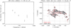 |
Fig. 1. For flare SOL2003-10-28T11:10: the flux density spectrum F(ν) showing the rising sub-THz component above 200 GHz (left panel), after Trottet et al. (2008) and UV solar flare ribbon observed by TRACE in the 1600 Å passband at 11:16:20 UT; 10 000 DN s−1 and 12 000 DN s−1 levels are shown as red and black contours (right panel). |
List of flares with a rising spectrum of sub-THz emission.
3. Ultraviolet observations of flare ribbons
Hard X-rays producing non-thermal electrons in flares deposit most of their energy in the chromosphere (Holman et al. 2011) leading to bright emission from the chromosphere and transition region and often faint HXR emission in the corona. Broadband UV images show flare ribbon emission from the transition region and chromosphere (e.g. Warren & Warshall 2001). To evaluate the flare ribbon area, we studied UV images at the 1600 Å passband, from the Transition Region and Coronal Explorer (TRACE; Handy et al. 1999) for seven flares before 2010 (the last TRACE science image was in 2010), and from the Solar Dynamics Observatory Atmospheric Imaging Assembly (SDO/AIA; Lemen et al. 2012) for ten flares after 2010. Both instruments provide adequate resolution; the TRACE pixel size is 0.5″ × 0.5″, and the AIA pixel size is 0.6″ × 0.6″. The time cadence for both instruments varies from 10–12 s to several minutes.
Because the considered flares are powerful (with GOES classes from M1.9 to X28), the UV images are usually saturated during the flare impulsive phase and the sub-THz emission peak. The saturation issue originates because pixels of the charge-couple device (CCD) are only able to accommodate a finite number of counts (Martinez et al. 1997), which can affect the intensity flux estimation. When pixels reach saturation level, spreading to adjacent pixels may begin, causing a secondary saturation (blooming). In turn, the blooming of the images can affect the area estimations. To recover saturated TRACE and AIA images, different approaches have been applied. Lin et al. (2001) offer the Solar SoftWare (SSW) routine trace_undiffract1 to clean TRACE images, while Schwartz et al. (2015) developed the DESAT package to de-saturate SDO/AIA images. Unfortunately both routines are only valid for a limited number of wavelengths (for TRACE: only for 171, 195, 284 Å; for AIA: 94, 131, 171, 193, 211, 304, 335 Å), and not for 1600 Å. In a statistical study of 190 flares observed with TRACE, Li & Zhang (2009) defined the uncertainty of the outer ribbon edges as a two-pixel error. To infer the ribbon-edge uncertainty, Kazachenko et al. (2012) defined different ribbon-edge cut-off values from six to ten times the background level.
In the current paper, we first define a cut-off range level and subtract the area of the saturated pixels affected by blooming to estimate the uncertainty on the flare areas. To remove saturation effects, the TRACE images have been processed with the SSW routine trace_prep.pro, which corrects for missing pixels, dark pedestal and current, and replaces saturated pixels with values above 4095 DN. A similar procedure, aia_prep.pro, has been applied to AIA images. The UV images are analysed at a time when sub-THz emission peaks or a few minutes before or after the peak if no other images are available or if they are saturated (see Tables 1 and 2). To define the area, we chose two levels which correspond to the maximum and minimum areas, normalised by the exposure time intensity, of Imin = 2000 DN s−1 and Imax = 4000 DN s−1, respectively. The areas of the found contours should not be less than 10 arcsec2, to exclude individual pixels and transient non-flare features (see Fig. 1 for an example). The UV areas AUV that satisfy the above requirements are summarised in Tables 1 and 2. Three flares (SOL2000-03-22, SOL2003-10-28, SOL2006-12-06), recorded by TRACE, have minimum and maximum levels of intensity at 10 000 and 12 000 DN s−1, respectively, since the count rate is extremely high.
List of flares with a decreasing spectrum of sub-THz emission.
4. UV flare ribbon areas and the sub-THz radio flux
The observed spectral flux density F(ν) [1 sfu = 10−22 W m−2 Hz−1] is proportional to the area of the emitting source and is given by the Rayleigh-Jeans relation
![Mathematical equation: $$ \begin{aligned} F=\frac{2\nu ^{2}k_{\rm B}T}{c^{2}}\frac{A}{R^{2}}\simeq 722\left(\frac{\nu }{100\,\mathrm{GHz}}\right)^{2} \left({\frac{T}{10^{6}\,\mathrm{K}}}\right) \left({\frac{A}{10^{3}\,\mathrm{arcsec}^{2}}}\right)~\mathrm{[sfu]}, \end{aligned} $$](/articles/aa/full_html/2018/12/aa34124-18/aa34124-18-eq19.gif) (1)
(1)
where kB is the Boltzmann constant, ν is the frequency, c is the speed of light, T is the temperature, A is the projected area of the radio source, and R is the Sun–Earth distance. Therefore, area A (Eq. (1)) is an important parameter for a thermal emission model. If the sub-THz emission originates from optically thick thermal plasma in the upper chromosphere/transition region, the area of the heated plasma should be proportional to the radio flux F ∝ AUV. Figure 2 shows the dependence of radio flux density F(ν) as a function of area AUV for 212 and 405 GHz, for the 14 solar flares with a positive spectral slope (Table 1). The area uncertainties for TRACE and AIA correspond to the maximum and minimum areas. Figure 2 demonstrates that all radio-fluxes between 200 and 400 GHz can be explained by radiation from an optically thick plasma with a temperature between 2 × 10⁴ K and 2 × 10⁶ K, which is the typical plasma temperature range for the transition region.
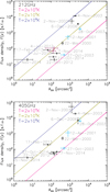 |
Fig. 2. Spectral flux density F(ν) vs. UV ribbon area AUV for 212 GHz (top panel) and 405 GHz (bottom panel) for flares with a positive spectral slope (9 events, black crosses and dates). For flares recorded at 230 and 345 GHz the fluxes were recalculated as F230 GHz/(2302)×(2122) and F345 GHz/(3452)×(4052), respectively (3 events, blue crosses and dates). For two flares registered at 93 and 140 GHz the fluxes were recalculated in a similar way to ν = 212 GHz and are shown only in the upper panel (2 events, purple crosses and dates). The flux density (solid lines) predicted by black-body emission for temperatures T = 2 × 10⁴, 2 × 10⁵, 2 × 10⁶ K are shown by pink, dark yellow, and dark blue lines, respectively. |
4.1. Thermal optically thick emission
The observations demonstrate that flares with larger radio fluxes tend to have larger UV ribbon areas (Fig. 2). In order to explain the highest observed radio flux density of ∼104 sfu, the temperature of the plasma should be 105 − 106 K, even for the brightest flares in October 2003 (Fig. 1). The radio flux increasing with increasing frequency would require an optically thick source. The optical depth τν over distance l can be written as
 (2)
(2)
where K = 9.78 × 10−3 × (18.2 + lnT3/2 − lnν) for T < 2 × 10⁵ K and K = 9.78 × 10−3 × (24.5 + lnT − lnν) for T > 2 × 10⁵ K (Dulk 1985). The above equation can be rewritten for an optical depth of τν = 1 to express the density ne required to provide optically thick emission
 (3)
(3)
For example, if the transition region is only 0.1 arcsec (∼72 km) thick, the plasma at a temperature of 105 K which is optically thick at 405 GHz should have density of 3 × 1012 cm−3 (Fig. 3).
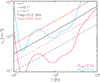 |
Fig. 3. Electron number density ne vs. temperature for T = 104 − 106 K, τ = 1, and a geometrical depth of l = 0.1″ (solid lines) and l = 1″ (dashed lines) for ν = 212 (black) and 405 GHz (red). The pink and blue lines indicate ne for the radiative loss times of Δtrad = 0.5, 0.1 s, respectively. |
4.2. HXR flare footpoints and sub-THz emission
RHESSI observations provide energy-dependent locations of HXR footpoints. HXR sources are found (Kontar et al. 2008, 2010; Saint-Hilaire et al. 2010) at heights around 0.7 − 1.7 Mm above the photospheric level. HXR emission of 30 keV is observed to be produced at heights of ∼1.7 Mm (Kontar et al. 2008), where the plasma density exceeds 1012 − 1013 cm−3, and co-spatial with white-light emission indicating ionisation caused by the non-thermal electrons (Battaglia & Kontar 2011, 2012). These observations suggest that sub-THz emission is located in a region where non-thermal electrons with energy < 30 keV are depositing their energy and the plasma densities are sufficient to make 0.4 THz emission optically thick. The observation of ribbon-like HXR emission (Liu et al. 2007) is often viewed as an additional indication that UV emission is caused by the energy deposition of HXR producing electrons.
4.3. Time variability of sub-THz emission
Relatively dense plasma n > 1011 cm−3 heated by energetic electrons to temperatures 0.1–1 MK leads to enhanced radiation (Raymond et al. 1976; Johnson et al. 2011; Scullion et al. 2016), so that the radiation losses would lead to effective cooling. The radiative cooling time is (Cox & Tucker 1969; Raymond et al. 1976; Bian et al. 2016)
 (4)
(4)
where the radiative loss function is calculated using the CHIANTI (Dere et al. 1997) function rad_loss.pro2. The radiative loss can be estimated using the approximation Λ(T)≃1.2 × 10⁻¹⁹ T−1/2, where T is in units of kelvin and Λ(T) in units of [erg cm 3 s−1], giving Λ(T)≃4 × 10⁻²² for T = 105 K.
The radiative loss time for plasma temperatures between T = 104 − 106 K is shown in Fig. 3. The results suggest that the plasma can quickly cool if the heating time is greater than the radiation loss time. The observations by Kaufmann et al. (2009a) show that the flux changes with a characteristic time of 0.1 − 1 s. This suggests that the interplay between non-thermal electron heating and the radiative cooling of dense plasma can explain the observed variability of sub-THz emission.
Quasi-synchronised broadband solar flare rapid pulsations at sub-second timescales are observed at HXR and centimetre-millimetre wavelengths (Takakura et al. 1983; Cornell et al. 1984; Kaufmann et al. 2000). These short-timescale features are often called “elementary bursts” following de Jager & de Jonge (1978). In particular, efforts to search for small-scale structures have also been made in optical wavelengths, typically Hα observations (Wang et al. 2000; Trottet et al. 2000; Kurt et al. 2000; Altyntsev et al. 2008; Fleishman et al. 2016) For example, Wang et al. (2000) reported fine temporal structures of the order of 0.3 − 0.7 s in Hα off-band emission, and it is found that these fine structures only occur at flare kernels whose light curves are closely correlated with HXR emission. This close correlation suggests that the sub-THz pulsations are caused by fast electron energy deposition or by thermal conduction in the transition region and heated chromosphere. In such a scenario, the finite temperature of the ambient plasma plays an important role in determining the energy deposition (Kontar et al. 2015; Jeffrey et al. 2015). An alternative way proposes heating by fast electrons accelerated in situ in the chromosphere due to the magnetic Rayleigh-Taylor instability (Zaitsev & Stepanov 2015, 2017).
5. The sub-THz emission model
During solar flares the transition region defined as the plasma between the chromosphere and corona (Tandberg-Hanssen et al. 1983) has a complicated structure. It can be viewed as an envelope covering the cool evaporating chromospheric plasma (Tandberg-Hanssen et al. 1983). This can be seen in limb flares where the dense chromospheric plasma expands into corona, so the transition region becomes vertically extended to coat this plasma. Moreover, a substantial vertical enhancement of the plasma density is required to explain the RHESSI observations (Kontar et al. 2010) and is visible in chromospheric evaporation simulations (e.g. Machado et al. 1980; Kašparová et al. 2009).
While the spectrum decreasing with frequency is a continuation of the standard gyrosynchrotron spectrum into the sub-THz range (Dulk 1985), the frequency-growing spectrum requires a different mechanism. For example, SOL2001-08-25T16:45 observed by Raulin et al. (2004) gives a large radio flux (5500 sfu) at 400 GHz, but it is consistent with the gyrosynchrotron spectrum decreasing with frequency that hides thermal emission. As a model to explain the radio emission growing with frequency, we propose that the large fluxes of sub-THz emission are due to the large areas of these flare ribbons. Therefore, the sub-THz flare component is produced at the heated flare ribbons and flares with small ribbon areas should produce weaker sub-THz emission, while the flares demonstrating extended flare ribbons should be strong sub-THz emitters. Then, the thermal emission from an optically thick transition region and low coronal plasma, with temperatures between 0.1 and 2 MK will produce a spectrum growing with frequency F(ν)∝να, where α ≤ 2.
In this scenario, the energy deposition rate is balanced by effective thermal radiative losses. As the plasma cools down quickly, the radio emission will stop as soon as the energy supply has ended. Variations in the electron acceleration rates will also produce radio flux variations at the timescales of radiation cooling (0.1 − 1 s) and provide a viable explanation for the sub-second variations of the flux (Kaufmann et al. 2009a).
Our model predicts that when the flare is compact (i.e. its UV ribbons have a small area) then the sub-THz radio flux is also small. We found observational support of this prediction. Table 2 shows that powerful GOES X-class flares can be weak emitters of sub-THz radiation. Although the flares have a GOES class of M and X, they are weak sub-THz flares. The peak of their radio flux is of the order of ∼100 sfu, and they have small ribbon areas not exceeding 500 arcsec2. Figure 2 also demonstrates that there is a smooth transition from flares with weak sub-THz emission to flares where the 400 GHz flux density exceeds 104 sfu, suggesting the same emission mechanism for all flares.
It is interesting to note that the model is also supported by observations of transition region lines. Ultraviolet observations of the transition region during flares show good correlation with HXR emission, which means that individual peaks in HXRs can be identified with individual peaks of UV emission (Tandberg-Hanssen et al. 1983; Warren & Warshall 2001). The ratios of transition region lines indicate (Raymond et al. 2007) that the emitting region is about 100 km thick for densities of the order of 1012 cm−3, similar to the densities required for the sub-THz emission (see Fig. 3).
6. Summary
We have examined solar flares that produce strong sub-THz emission rising with frequency. Flares with strong radiation in the sub-THz frequency range tend to have large and extended flare ribbon areas, clearly seen in UV.
To explain the observations, we propose that the rising component of the sub-THz radiation is produced via thermal bremsstrahlung (free-free emission) from an optically thick plasma located in the transition region heated by precipitating non-thermal electrons, ions or heat conduction. Due to flare heating of the chromosphere, the plasma evaporates and fills the loop, forcing the transition region to lower heights (Hirayama 1974) and hence higher density regions (Machado et al. 1980; Kašparová et al. 2009), where radio emission with ν < 0.4 THz emission becomes optically thick. Plasma in the range of temperatures of 0.1–1 MK then produces enhanced sub-THz emission. The model provides a frequency spectrum that grows with frequency, for flares with ribbon areas of ∼1000 arcsec2, which produces a radio flux density of 104 sfu (Kaufmann 2012). We note that the quiet-Sun transition region is located at an altitude of ∼2 Mm with a plasma density of 1011 cm−3 (Vernazza et al. 1981) and it is optically thin to such radio emission, so the sub-THz emission is produced in the chromosphere where the plasma temperature is < 104 K. It should be noted that in the presence of strong gyrosynchrotron emission, the flux in the sub-THz range could be dominated by this gyrosynchrotron component producing smaller radio source sizes. In particular, the observations by Lüthi et al. (2004b) are consistent with the gyrosynchrotron source dominating 210 GHz observations, while the gyrosynchrotron emission dominates up to 400 GHz in SOL2001-08-25.
The rapid heating by non-thermal electrons with energy ∼20 keV and radiative cooling of the dense > 1012 cm−3 plasma is likely to produce variations at sub-second timescales and this should be temporarily correlated with the HXR flux of electrons and/or ions, the particles that produce evaporation, and hence an enhanced density of heated evaporating plasma.
In summary, we have analysed virtually all flares with a rising sub-THz component reported in the literature. We analysed UV ribbon areas, a signature of energy deposition in the chromosphere, and the observational results suggest that the strong sub-THz emission is associated with large UV ribbon areas. Large flare ribbon areas can explain this sub-THz emission as the thermal emission from optically thick plasma with a temperature of 0.1–2 MK. Our model is consistent with the standard solar flare scenario and shows that the sub-THz emission could be a valuable temperature diagnostic tool of the dynamic transition region during solar flares.
Acknowledgments
EPK is indebted to P. Kaufmann for the inspiring discussions and hospitality in São Paulo, Brazil. EPK and NLSJ gratefully acknowledge the financial support from the STFC Consolidated Grant ST/L000741/1. GM is supported by the Russian Science Foundation (project no. 16-12-10448).
References
- Altyntsev, A. T., Fleishman, G. D., Huang, G.-L., & Melnikov, V. F. 2008, ApJ, 677, 1367 [NASA ADS] [CrossRef] [Google Scholar]
- Aschwanden, M. J., Caspi, A., Cohen, C. M. S., et al. 2017, ApJ, 836, 17 [NASA ADS] [CrossRef] [Google Scholar]
- Battaglia, M., & Kontar, E. P. 2011, A&A, 533, L2 [NASA ADS] [CrossRef] [EDP Sciences] [Google Scholar]
- Battaglia, M., & Kontar, E. P. 2012, ApJ, 760, 142 [NASA ADS] [CrossRef] [Google Scholar]
- Benz, A. O. 2008, Liv. Rev. Sol. Phys., 5, 1 [Google Scholar]
- Bian, N. H., Watters, J. M., Kontar, E. P., & Emslie, A. G. 2016, ApJ, 833, 76 [NASA ADS] [CrossRef] [Google Scholar]
- Cornell, M. E., Hurford, G. J., Kiplinger, A. L., & Dennis, B. R. 1984, ApJ, 279, 875 [NASA ADS] [CrossRef] [Google Scholar]
- Cox, D. P., & Tucker, W. H. 1969, ApJ, 157, 1157 [NASA ADS] [CrossRef] [Google Scholar]
- de Jager, C., & de Jonge, G. 1978, Sol. Phys., 58, 127 [NASA ADS] [CrossRef] [Google Scholar]
- Dere, K. P., Landi, E., Mason, H. E., Monsignori Fossi, B. C., & Young, P. R. 1997, A&AS, 125, 149 [NASA ADS] [CrossRef] [EDP Sciences] [Google Scholar]
- Dulk, G. A. 1985, ARA&A, 23, 169 [NASA ADS] [CrossRef] [Google Scholar]
- Fernandes, L. O. T., Kaufmann, P., Correia, E., et al. 2017, Sol. Phys., 292, 21 [NASA ADS] [CrossRef] [Google Scholar]
- Fleishman, G. D., & Kontar, E. P. 2010, ApJ, 709, L127 [NASA ADS] [CrossRef] [Google Scholar]
- Fleishman, G. D., Pal’shin, V. D., Meshalkina, N., et al. 2016, ApJ, 822, 71 [NASA ADS] [CrossRef] [Google Scholar]
- Handy, B. N., Acton, L. W., Kankelborg, C. C., et al. 1999, Sol. Phys., 187, 229 [NASA ADS] [CrossRef] [Google Scholar]
- Hirayama, T. 1974, Sol. Phys., 34, 323 [NASA ADS] [CrossRef] [Google Scholar]
- Holman, G. D., Aschwanden, M. J., Aurass, H., et al. 2011, Space Sci. Rev., 159, 107 [NASA ADS] [CrossRef] [Google Scholar]
- Jeffrey, N. L. S., Kontar, E. P., Emslie, A. G., & Bian, N. H. 2015, J. Phys. Conf. Ser., 642, 012013 [NASA ADS] [CrossRef] [Google Scholar]
- Johnson, H., Raymond, J. C., Murphy, N. A., et al. 2011, ApJ, 735, 70 [NASA ADS] [CrossRef] [Google Scholar]
- Kaufmann, P. 2012, Astrophys. Space Sci. Proc., 30, 61 [NASA ADS] [CrossRef] [Google Scholar]
- Kaufmann, P., Trottet, G., Giménez de Castro, C. G., et al. 2000, Sol. Phys., 197, 361 [NASA ADS] [CrossRef] [Google Scholar]
- Kaufmann, P., Raulin, J.-P., Correia, E., et al. 2001, ApJ, 548, L95 [NASA ADS] [CrossRef] [Google Scholar]
- Kaufmann, P., Raulin, J.-P., de Castro, C. G. G., et al. 2004, ApJ, 603, L121 [NASA ADS] [CrossRef] [Google Scholar]
- Kaufmann, P., Giménez de Castro, C. G., Correia, E., et al. 2009a, ApJ, 697, 420 [NASA ADS] [CrossRef] [Google Scholar]
- Kaufmann, P., Trottet, G., Giménez de Castro, C. G., et al. 2009b, Sol. Phys., 255, 131 [NASA ADS] [CrossRef] [Google Scholar]
- Kašparová, J., Heinzel, P., Karlický, M., Moravec, Z., & Varady, M. 2009, Cent. Eur. Astrophys. Bull., 33, 309 [NASA ADS] [Google Scholar]
- Kazachenko, M. D., Canfield, R. C., Longcope, D. W., & Qiu, J. 2012, Sol. Phys., 277, 165 [NASA ADS] [CrossRef] [Google Scholar]
- Klopf, J. M., Kaufmann, P., Raulin, J.-P., & Szpigel, S. 2014, ApJ, 791, 31 [NASA ADS] [CrossRef] [Google Scholar]
- Kontar, E. P., Hannah, I. G., & MacKinnon, A. L. 2008, A&A, 489, L57 [NASA ADS] [CrossRef] [EDP Sciences] [Google Scholar]
- Kontar, E. P., Hannah, I. G., Jeffrey, N. L. S., & Battaglia, M. 2010, ApJ, 717, 250 [NASA ADS] [CrossRef] [Google Scholar]
- Kontar, E. P., Brown, J. C., Emslie, A. G., et al. 2011, Space Sci. Rev., 159, 301 [NASA ADS] [CrossRef] [Google Scholar]
- Kontar, E. P., Jeffrey, N. L. S., Emslie, A. G., & Bian, N. H. 2015, ApJ, 809, 35 [NASA ADS] [CrossRef] [Google Scholar]
- Kontar, E. P., Perez, J. E., Harra, L. K., et al. 2017, Phys. Rev. Lett., 118, 155101 [NASA ADS] [CrossRef] [Google Scholar]
- Krucker, S., Giménez de Castro, C. G., Hudson, H. S., et al. 2013, A&ARv, 21, 58 [NASA ADS] [CrossRef] [Google Scholar]
- Kurt, V. G., Akimov, V. V., Hagyard, M. J., & Hathaway, D. H. 2000, in High Energy Solar Physics Workshop – Anticipating Hess!, eds. R. Ramaty, & N. Mandzhavidze, ASP Conf. Ser., 206, 426 [NASA ADS] [Google Scholar]
- Lemen, J. R., Title, A. M., Akin, D. J., et al. 2012, Sol. Phys., 275, 17 [NASA ADS] [CrossRef] [Google Scholar]
- Li, L., & Zhang, J. 2009, ApJ, 690, 347 [NASA ADS] [CrossRef] [Google Scholar]
- Lin, A. C., Nightingale, R. W., & Tarbell, T. D. 2001, Sol. Phys., 198, 385 [NASA ADS] [CrossRef] [Google Scholar]
- Lin, R. P., Dennis, B. R., Hurford, G. J., et al. 2002, Sol. Phys., 210, 3 [Google Scholar]
- Liu, C., Lee, J., Gary, D. E., & Wang, H. 2007, ApJ, 658, L127 [NASA ADS] [CrossRef] [Google Scholar]
- Lüthi, T., Magun, A., & Miller, M. 2004a, A&A, 415, 1123 [NASA ADS] [CrossRef] [EDP Sciences] [Google Scholar]
- Lüthi, T., Lüdi, A., & Magun, A. 2004b, A&A, 420, 361 [NASA ADS] [CrossRef] [EDP Sciences] [Google Scholar]
- Machado, M. E., Avrett, E. H., Vernazza, J. E., & Noyes, R. W. 1980, ApJ, 242, 336 [NASA ADS] [CrossRef] [Google Scholar]
- Martinez, P., Klotz, A., Demers, A., Léna, F., & b. P., 1997, A Practical Guide to CCD Astronomy (Cambridge, UK: Cambridge University Press), 263 [Google Scholar]
- Raulin, J. P., Makhmutov, V. S., Kaufmann, P., et al. 2004, Sol. Phys., 223, 181 [NASA ADS] [CrossRef] [Google Scholar]
- Raymond, J. C., Cox, D. P., & Smith, B. W. 1976, ApJ, 204, 290 [NASA ADS] [CrossRef] [Google Scholar]
- Raymond, J. C., Holman, G., Ciaravella, A., et al. 2007, ApJ, 659, 750 [NASA ADS] [CrossRef] [Google Scholar]
- Saint-Hilaire, P., Krucker, S., & Lin, R. P. 2010, ApJ, 721, 1933 [NASA ADS] [CrossRef] [Google Scholar]
- Sakai, J. I., Nagasugi, Y., Saito, S., & Kaufmann, P. 2006, A&A, 457, 313 [NASA ADS] [CrossRef] [EDP Sciences] [Google Scholar]
- Schwartz, R. A., Torre, G., Massone, A. M., & Piana, M. 2015, Astron. Comput., 13, 117 [NASA ADS] [CrossRef] [Google Scholar]
- Scullion, E., Rouppe van der Voort, L., Antolin, P., et al. 2016, ApJ, 833, 184 [NASA ADS] [CrossRef] [Google Scholar]
- Silva, A. V. R., Share, G. H., Murphy, R. J., et al. 2007, Sol. Phys., 245, 311 [NASA ADS] [CrossRef] [Google Scholar]
- Takakura, T., Kaufmann, P., Costa, J. E. R., et al. 1983, Nature, 302, 317 [NASA ADS] [CrossRef] [Google Scholar]
- Tandberg-Hanssen, E., Reichmann, E., & Woodgate, B. 1983, Sol. Phys., 86, 159 [NASA ADS] [CrossRef] [Google Scholar]
- Trottet, G., & Klein, K.-L. 2013, Mem. Soc. Astron. It., 84, 405 [NASA ADS] [Google Scholar]
- Trottet, G., Rolli, E., Magun, A., et al. 2000, A&A, 356, 1067 [NASA ADS] [Google Scholar]
- Trottet, G., Raulin, J.-P., Kaufmann, P., et al. 2002, A&A, 381, 694 [NASA ADS] [CrossRef] [EDP Sciences] [Google Scholar]
- Trottet, G., Krucker, S., Lüthi, T., & Magun, A. 2008, ApJ, 678, 509 [NASA ADS] [CrossRef] [Google Scholar]
- Trottet, G., Raulin, J.-P., Giménez de Castro, G., et al. 2011, Sol. Phys., 273, 339 [NASA ADS] [CrossRef] [Google Scholar]
- Tsap, Y. T., Smirnova, V. V., Morgachev, A. S., et al. 2016, Adv. Space Res., 57, 1449 [NASA ADS] [CrossRef] [Google Scholar]
- Tsap, Y. T., Smirnova, V. V., Motorina, G. G., et al. 2018, Sol. Phys., 293, 50 [NASA ADS] [CrossRef] [Google Scholar]
- Vernazza, J. E., Avrett, E. H., & Loeser, R. 1981, ApJS, 45, 635 [NASA ADS] [CrossRef] [Google Scholar]
- Wang, H., Qiu, J., Denker, C., et al. 2000, ApJ, 542, 1080 [NASA ADS] [CrossRef] [Google Scholar]
- Warren, H. P., & Warshall, A. D. 2001, ApJ, 560, L87 [NASA ADS] [CrossRef] [Google Scholar]
- Zaitsev, V. V., & Stepanov, A. V. 2015, Sol. Phys., 290, 3559 [NASA ADS] [CrossRef] [Google Scholar]
- Zaitsev, V. V., & Stepanov, A. V. 2017, Sol. Phys., 292, 141 [NASA ADS] [CrossRef] [Google Scholar]
- Zaitsev, V. V., Stepanov, A. V., & Melnikov, V. F. 2013, Astron. Lett., 39, 650 [NASA ADS] [CrossRef] [Google Scholar]
- Zaitsev, V. V., Stepanov, A. V., & Kaufmann, P. 2014, Sol. Phys., 289, 3017 [NASA ADS] [CrossRef] [Google Scholar]
All Tables
All Figures
|
Fig. 1. For flare SOL2003-10-28T11:10: the flux density spectrum F(ν) showing the rising sub-THz component above 200 GHz (left panel), after Trottet et al. (2008) and UV solar flare ribbon observed by TRACE in the 1600 Å passband at 11:16:20 UT; 10 000 DN s−1 and 12 000 DN s−1 levels are shown as red and black contours (right panel). |
| In the text | |
|
Fig. 2. Spectral flux density F(ν) vs. UV ribbon area AUV for 212 GHz (top panel) and 405 GHz (bottom panel) for flares with a positive spectral slope (9 events, black crosses and dates). For flares recorded at 230 and 345 GHz the fluxes were recalculated as F230 GHz/(2302)×(2122) and F345 GHz/(3452)×(4052), respectively (3 events, blue crosses and dates). For two flares registered at 93 and 140 GHz the fluxes were recalculated in a similar way to ν = 212 GHz and are shown only in the upper panel (2 events, purple crosses and dates). The flux density (solid lines) predicted by black-body emission for temperatures T = 2 × 10⁴, 2 × 10⁵, 2 × 10⁶ K are shown by pink, dark yellow, and dark blue lines, respectively. |
| In the text | |
|
Fig. 3. Electron number density ne vs. temperature for T = 104 − 106 K, τ = 1, and a geometrical depth of l = 0.1″ (solid lines) and l = 1″ (dashed lines) for ν = 212 (black) and 405 GHz (red). The pink and blue lines indicate ne for the radiative loss times of Δtrad = 0.5, 0.1 s, respectively. |
| In the text | |
Current usage metrics show cumulative count of Article Views (full-text article views including HTML views, PDF and ePub downloads, according to the available data) and Abstracts Views on Vision4Press platform.
Data correspond to usage on the plateform after 2015. The current usage metrics is available 48-96 hours after online publication and is updated daily on week days.
Initial download of the metrics may take a while.