| Issue |
A&A
Volume 619, November 2018
|
|
|---|---|---|
| Article Number | A168 | |
| Number of page(s) | 19 | |
| Section | Extragalactic astronomy | |
| DOI | https://doi.org/10.1051/0004-6361/201833727 | |
| Published online | 21 November 2018 | |
Broad-line region structure and line profile variations in the changing look AGN HE 1136-2304⋆
1 Institut für Astrophysik, Universität Göttingen, Friedrich-Hund Platz 1, 37077 Göttingen, Germany
e-mail: This email address is being protected from spambots. You need JavaScript enabled to view it.
2 Astronomisches Institut, Ruhr-Universität Bochum, Universitätsstrasse 150, 44801 Bochum, Germany
3 Physics Department and the Haifa Research Center for Theoretical Physics and Astrophysics, University of Haifa, Haifa, 3498838, Israel
4 School of Physics & Astronomy and the Wise Observatory, The Raymond and Beverly Sackler Faculty of Exact Sciences Tel-Aviv University, Tel-Aviv, 69978, Israel
5 Department of Earth and Space Sciences, Morehead State University, Morehead, KY, 40351, USA
Received:
27
June
2018
Accepted:
7
August
2018
Abstract
Aims. A strong X-ray outburst was detected in HE 1136-2304 in 2014. Accompanying optical spectra revealed that the spectral type has changed from a nearly Seyfert 2 type (1.95), classified by spectra taken 10 and 20 years ago, to a Seyfert 1.5 in our most recent observations. We seek to investigate a detailed spectroscopic campaign on the spectroscopic properties and spectral variability behavior of this changing look AGN and compare this to other variable Seyfert galaxies.
Methods. We carried out a detailed spectroscopic variability campaign of HE 1136-2304 with the 10 m Southern African Large Telescope (SALT) between 2014 December and 2015 July.
Results. The broad-line region (BLR) of HE 1136-2304 is stratified with respect to the distance of the line-emitting regions. The integrated emission line intensities of Hα, Hβ, He I λ5876, and He II λ4686 originate at distances of 15.0−3.8+4.2, 7.5−5.7+4.6, 7.3−4.4+2.8, and 3.0−3.7+5.3 light days with respect to the optical continuum at 4570 Å. The variability amplitudes of the integrated emission lines are a function of distance to the ionizing continuum source as well. We derived a central black hole mass of 3.8 ± 3.1 × 10⁷ M⊙ based on the linewidths and distances of the BLR. The outer line wings of all BLR lines respond much faster to continuum variations indicating a Keplerian disk component for the BLR. The response in the outer wings is about two light days shorter than the response of the adjacent continuum flux with respect to the ionizing continuum flux. The vertical BLR structure in HE 1136-2304 confirms a general trend that the emission lines of narrow line active galactic nuclei (AGNs) originate at larger distances from the midplane in comparison to AGNs showing broader emission lines. Otherwise, the variability behavior of this changing look AGN is similar to that of other AGN.
Key words: galaxies: active / galaxies: Seyfert / galaxies: nuclei / galaxies: individual: HE 1136-2304 / quasars: emission lines
Based on observations obtained with the Southern African Large Telescope.
© ESO 2018
1. Introduction
About a dozen Seyfert galaxies are known to have significantly changed their optical spectral type: for example, NGC 3515 (Collin-Souffrin et al. 1973), NGC 4151 (Penston & Perez 1984), Fairall 9 (Kollatschny & Fricke 1985), NGC 2617 (Shappee et al. 2014), Mrk 590 (Denney et al. 2014); and references therein. Further recent findings are based on spectral variations detected by means of the Sloan Digital Sky Survey (e.g., Komossa et al. 2008; LaMassa et al. 2015; Runnoe et al. 2016; MacLeod et al. 2016). These galaxies are considered to be changing look active galactic nuclei (AGNs). However, most of these findings are based on only a few spectra.
HE 1136-2304 (α2000 = 11h38m51.1s, δ = 23∘21′36′′, z = 0.0271) was classified as a changing look AGN based on spectroscopy performed after a strong increase in the X-ray flux was detected by XMM-Newton in 2014 in comparison to an upper limit based on the ROSAT All-Sky Survey taken in 1990 (Parker et al. 2016). The increase in the X-ray flux came with an increase in the optical continuum flux and with a change of the Seyfert type. HE 1136-2304 was of Seyfert 2/1.95 type in early spectra taken in 1993 and 2002. However, its spectral type changed to a Seyfert 1.5 type in 2014 (Zetzl et al. 2018, Paper I). This notation of Seyfert subclasses was introduced by Osterbrock (1981).
Long-term and detailed optical variability studies exist for many AGN such as NGC 5548 (Peterson et al. 2002; Pei et al. 2017; and references therein), 3C120 (Peterson et al. 1998; Kollatschny et al. 2000; Grier et al. 2013), NGC 7603 (Kollatschny et al. 2000), and 3C 390.3 (Shapovalova et al. 2010). Corresponding detailed follow-up studies have not yet been reported for the type of changing look AGN mentioned above.
We carried out a detailed spectroscopic and photometric variability study of HE 1136-2304 between 2014 and 2015 after the detection of the strong outburst in 2014. We presented the optical, UV, and X-ray continuum variations of HE 1136-2304 from 2014 to 2017 in a separate paper (Paper I). We verified strong continuum variations in the X-ray, UV, and optical continua. We showed that the variability amplitude decreased with increasing wavelength. The amplitude in the optical varied by a factor of three after correcting for the host galaxy contribution. No systematic trends were found with regards to the variability behavior following the outburst in 2014. A general decrease in flux would have been expected for a tidal disruption event. The Seyfert type did not change between 2014 and 2017 despite strong continuum variations. We describe the results of the spectroscopic variability campaign taken with the 10 m Southern African Large Telescope (SALT) for the years 2014–2015.
Throughout this paper, we assume Λ cold dark matter cosmology with a Hubble constant of H0 = 70 km s−1 Mpc−1, ΩM = 0.27, and ΩΛ = 0.73. Following the cosmological calculator by (Wright 2006) this results in a luminosity distance of 118 Mpc.
2. Observations and data reduction
In addition to our first spectrum obtained on 2014 July 7 (Parker et al. 2016), we took optical spectra of the Seyfert galaxy HE 1136-2304 with the SALT at 17 epochs between 2014 December 25 and 2015 July 13. The log of our spectroscopic observations is given in Table 1.
Log of spectroscopic observations of HE 1136-2304 with SALT.
The spectra taken of HE 1136-2304 between 2015 February and 2015 July had a mean interval of nine days. For some epochs spectra were acquired at shorter intervals.
All spectroscopic observations were taken with identical instrumental setups. We used the Robert Stobie Spectrograph attached to the SALT using the PG0900 grating. The slit width was fixed to 2′′.0 projected on the sky at an optimized position angle to minimize differential refraction. Furthermore, all observations were taken at the same airmass owing to the particular design of the SALT. The spectra were taken with exposure times of 16–20 min.
Typical seeing values were 1–2 arcsec. We covered a wavelength range from 4355 Å to 7230 Å, which corresponds to a rest-frame wavelength range of 4240 Å–7040 Å. The spectral resolution was 6.5 Å. There are two gaps in the spectrum caused by the gaps between the three CCDs: one between the blue and the central CCD chip and one between the central and red CCD chip covering the wavelengths in the ranges 5206–5263 Å and 6254–6309 Å (5069–5124 Å and 6089–6142 Å in the rest frame). All spectra shown in this work were shifted to the rest frame of HE 1136-2304.
In addition to the galaxy spectrum, necessary flat-field and Xe arc frames were also observed, as well as spectrophotometric standard stars for flux calibration (LTT3218, LTT7379, and EG274). Flat-field frames were used to correct for differences in sensitivity both between detector pixels and across the field. The spatial resolution per binned pixel was 0′′.2534 for our SALT spectrum. We extracted eight columns from the object spectrum corresponding to 2′′.03.
We reduced the spectra (bias subtraction, cosmic ray correction, flat-field correction, 2D-wavelength calibration, night sky subtraction, and flux calibration) in a homogeneous way with the Image Reduction and Analysis Facility (IRAF) reduction packages (e.g., Kollatschny et al. 2001). Great care was taken to ensure high-quality intensity and wavelength calibrations to keep the intrinsic measurement errors very low (Kollatschny et al. 2001; Kollatschny 2003; Kollatschny & Zetzl 2010). The spectra of HE1136-2304 and the calibration star spectra were not always taken under photometric conditions. Therefore, all spectra were calibrated to the same absolute [O III] λ5007 flux of 1.75 × 10⁻¹³ erg s−1 cm−2 (Reimers et al. 1996). The flux of the narrow emission line [O III] λ5007 is considered to be constant on timescales of years. The accuracy of the [O III] λ5007 flux calibration was tested for all forbidden emission lines in the spectra. We calculated difference spectra for all epochs with respect to the mean spectrum of our variability campaign. Corrections for both small spectral shifts (< 0.5 Å) and small scaling factors were executed by minimizing the residuals of the narrow emission lines in the difference spectra. A relative flux accuracy on the order of 1% was achieved for most of the spectra.
3. Results
3.1. Continuum and spectral line variations
We present all final reduced optical spectra of HE 1136-2304 taken during the 2014/2015 variability campaign in Fig. 1. These results clearly show variations in the continuum intensities. The mean and rms spectra of HE 1136-2304 are shown in Fig. 2. The rms spectrum presents the variable part of the emission lines. The spectrum was scaled by a factor of 6.9 to allow for a better comparison with the mean spectrum and for enhancing weaker line structures. We note that all wavelengths referred to in this section are rest-frame wavelengths.
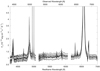 |
Fig. 1. Optical spectra of HE 1136-2304 taken with the SALT telescope for our variability campaign from December 2014 until July 2015. |
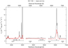 |
Fig. 2. Integrated mean (black) and rms (red) spectra for our variability campaign of HE 1136-2304. The rms spectrum has been scaled by a factor of 6.9 to enhance weak line structures. |
The integration limits of the broad emission lines and continuum regions are given at the bottom of the spectra. To select the continuum regions, we inspected the mean and rms spectra for regions that are free of both strong emission and absorption lines. The final wavelength ranges used for our continuum flux measurements are given in Table 2. A continuum region at 5100 Å is often used in studies of the variable continuum flux in AGN. Normally, this region is free of strong emission lines and close to the [O III] λ5007 flux calibration line. However, in our case this region falls in the gap between the blue and central CCD chip. Therefore we set a nearby continuum range at 5360 Å. In addition to this continuum range, we determined the continuum intensities at three additional ranges (at 4570, 6235, and 6835 Å; see Fig. 2 and Table 2). We used these continuum regions for creating pseudo-continua below the variable broad emission lines. We neglected a possible contribution of FeII blends to the continuum flux based on our mean and rms spectra.
Rest-frame continuum boundaries and line integration limits.
We integrated the broad Balmer and Helium emission-line intensities between the wavelength boundaries given in Table 2. Before integrating each emission line flux, we subtracted a linear pseudo-continuum defined by the boundaries given in Table 2 (Col. 3). We did not consider the Hγ line in our studies as it was not possible to determine a reliable continuum at the blue side of this line. The results of the continuum and line intensity measurements are given in Table 3. Additionally, we present in this table the flux values obtained for our first spectrum taken on 2014 July 7.
We present the light curves of the continuum fluxes at 4570 Å and 5360 Å as well as those of the integrated emission line fluxes of Hα, Hβ, He II λ4686, and He I λ5876 in Fig. 3. Some statistics of the emission line intensity and continuum variations are given in Table 4. We indicate the minimum and maximum fluxes Fmin and Fmax, peak-to-peak amplitudes Rmax = Fmax/Fmin, the mean flux over the period of observations ⟨F⟩, standard deviation σF, and fractional variation Fvar (see Paper I).
Continuum and integrated broad line fluxes for different epochs.
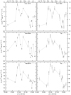 |
Fig. 3. Light curves of the continuum fluxes at 4570 Å and 5360 Å (in units of 10−15 erg cm−2 s−1 Å−1) as well as of the integrated emission line fluxes of Hα, Hβ, He II λ4686, and He I λ5876 (in units of 10−14 erg cm−2 s−1) for our variability campaign from 2014 December until 2015 July. |
Variability statistics based on the SALT data in units of 10−15 erg s−1 cm−2 Å−1 for the continuum as well as in units of 10−15 erg s−1 cm−2 for the emission lines.
We calculated the Balmer decrement Hα/Hβ of the broad components after subtraction of the narrow components for the individual epochs. The results are shown in Fig. 4 as a function of the continuum intensity at 4570 Å. Figure 5 gives the Balmer decrement as a function of the Hβ line intensity. The Balmer decrement Hα/Hβ of the broad components takes values between 3.5 and 7.5. On the other hand, we measure a constant value of 2.81 for the Balmer decrement Hα/Hβ of the narrow components. There is a clear trend that the Balmer decrement Hα/Hβ of the broad component decreases with increasing luminosity.
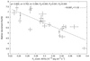 |
Fig. 4. Balmer decrement Hα/Hβ of the broad line components vs. the continuum intensity at 4570 Å. The dashed line on the graph represents the linear regression. |
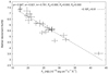 |
Fig. 5. Balmer decrement Hα/Hβ of the broad line components vs. broad line Hβ intensity. The dashed line on the graph represents the linear regression. |
3.2. Mean and rms line profiles
We determined normalized mean and rms profiles of the Balmer and Helium lines after subtracting the continuum fluxes in each individual spectrum using the continuum windows listed in Table 2. Figures 6–14 show the mean and rms profiles of the Balmer lines Hα and Hβ as well as those of the He lines He I λ5876 and He II λ4686 in velocity space. The rms profiles illustrate the line profile variations during our campaign. The constant narrow components disappear almost completely in these rms profiles. However, the mean profiles contain strong narrow line components in addition to their broad line components. We subtracted the narrow Balmer and Helium line components in all the mean profiles by subtracting a scaled [O III] λ5007 line profile as a template. Furthermore, we subtracted the narrow [N II] λ6584 line in the mean Hα profile and removed the [Fe III] λ4861 line in the mean He II λ4686 profile as well. After subtracting these narrow components we compared the mean and rms profiles of the broad emission lines with each other in a more accurate way.
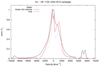 |
Fig. 6. Normalized mean (blue), mean without a narrow component (black), and rms (red) line profiles of Hα in velocity space. |
We present the normalized mean profiles (with and without narrow components) and rms profiles for all four Balmer and Helium emission lines in Figs. 6–9. A comparison of all normalized mean profiles including their narrow components is shown in Fig. 10. We then present a comparison of the mean profiles after subtracting the narrow components; this comparison is shown in Fig. 11 for the mean profiles of Hα and Hβ. For getting a hint on line asymmetries their flipped profiles at v = 0 km s−1 are depicted as well. Figure 12 presents the mean Helium profiles after subtracting their narrow components. The profile of Hβ has also been added for comparison purposes. Figure 13 shows a comparison of the Hα and Hβ rms line profiles normalized with respect to their central component. Again their flipped profiles at v = 0 km s−1 are depicted to highlight the additional strong red components and the weak blue component. Finally, Fig. 14 gives the rms profiles of the Helium lines. Again, the Hβ line profile has been added for comparison.
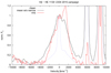 |
Fig. 7. Normalized mean (blue), mean without a narrow component (black), and rms (red) line profiles of Hβ in velocity space. |
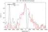 |
Fig. 8. Normalized mean (blue), mean without a narrow component (black), and rms (red) line profiles of He I λ5876 in velocity space. |
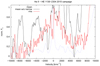 |
Fig. 9. Normalized mean (blue), mean without a narrow component (black), and rms (red) line profiles of He II λ4686 in velocity space. |
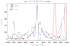 |
Fig. 10. Normalized mean line profiles of Hα, Hβ, He I λ5876, and He II λ4686. |
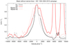 |
Fig. 11. Normalized mean line profiles of Hα, Hβ without a narrow component. In addition, we flipped the profiles at v = 0 km s−1. |
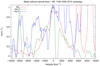 |
Fig. 12. Normalized mean line profiles of Hβ, He I λ5876, and He II λ4686 without a narrow component. |
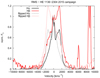 |
Fig. 13. Normalized rms line profiles of Hα, Hβ. In addition, we flipped the profiles at v = 0 km s−1. |
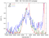 |
Fig. 14. Normalized rms line profiles of Hβ, He I λ5876, and He II λ4686. |
We determined the linewidths (FWHM) of the mean and rms line profiles of all the Balmer and Helium lines. These measurements were performed with respect to the maximum of the central component and are listed in Table 5. In addition, we parameterized the linewidths of the rms profiles by their line dispersion σline (rms widths; Fromerth & Melia 2000; Peterson et al. 2004). The Balmer line profiles (mean and rms) exhibit linewidths (FWHM) between 2500 and 4000 km s−1. Hα shows the narrowest broad line profiles. The Helium lines (He I λ5876 and He II λ4686) are always broader than the Balmer lines by 500–1500 km s−1. Furthermore, the outer blue wing is more extended in the higher ionized He lines in comparison to the Balmer lines (Figs. 13 and 14). This might be an indication of an additional outflowing component in the inner broad-line region (BLR).
Balmer and Helium linewidths: FWHM of the mean and rms line profiles as well as the line dispersion σline of the rms profiles.
An additional strong red component emerges in the rms and mean profiles of the Hα and Hβ lines at 1380 km s−1 and varies with a larger amplitude than the rest of the line profile. Furthermore, this component shows a relatively stronger variation in Hβ in comparison with Hα (see Fig. 13) by a factor of 1.5. An indication of the existence of this red component is present in the He II λ4686 line as well (Fig. 14). No clear indication of this component is visible in the red wing of the He I λ5876 line as that region coincides with the NaD absorption. An additional blue component, nearly symmetrical to the red component, appears in the rms profile of Hβ at around −1400 km s−1 (Fig. 13). However, this blue component is by far weaker than the red component. The existence of blue and red components in the line profiles – in addition to the central component – are an indication that the broad line-emitting region is connected with an accretion disk structure.
3.3. CCF analysis of the integrated broad emission lines
3.3.1. Based on SALT spectra
The mean distances of the broad emitting line regions to the central ionizing source can be determined by correlating the broad emission line light curves with the light curves of the ionizing continuum flux. Normally, an optical continuum light curve is used as a surrogate for the ionizing flux light curve. An interpolation cross-correlation function method (ICCF) has been developed by Gaskell & Peterson (1987) to calculate the delay of the individual line light curves with respect to the continuum light curve. We generated our own ICCF code (Dietrich & Kollatschny 1995) based on similar assumptions in the past. For this study, we correlated the light curves of the integrated Balmer (Hα, Hβ) and Helium lines (He I λ5876, He II λ4686) with the continuum light curve at 4570 Å using our method. The derived ICCF(τ) are presented in Fig. 15.
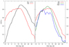 |
Fig. 15. Cross-correlation functions of the integrated Hα, Hβ, He I λ5876, and He II λ4686 lines with respect to the continuum at 4570 Å. |
We determined the centroids of these ICCF, τcent by using only those parts of the CCFs above 80% of the peak value rmax. A threshold value of 0.8 rmax is generally a good choice as had been shown by, for example, Peterson et al. (2004). We derived the uncertainties in our cross-correlation results by calculating the cross-correlation lags a large number of times using a model-independent Monte Carlo method known as flux redistribution/random subset selection (FR/RSS). This method has been described by Peterson et al. (1998). Here the error intervals correspond to 68% confidence levels. The final results of the ICCF analysis are given in Table 6.
Cross-correlation lags of the Balmer and Helium line light curves with respect to the 4570 Å continuum light curve.
The delay of the line-averaged BLR size of the integrated Balmer lines with respect to the continuum light curve at 4570 Å corresponds to  and
and  light days in the Hα and Hβ lines, respectively. The He I λ5876 shows a delay of
  days while the delay of the integrated He II λ4686 line corresponds to
  light days.
The CCF of Hβ is very broad in comparison to Hα (see Fig. 15). We discuss in Sect. 3.5 how individual segments of the emission lines exhibit different delays with respect to the ionizing continuum. The line wings originate closer to the central ionizing zone while the central line regions originate at larger distances from the central ionizing zone. We carried out additional tests whether the integrated inner line profile segments (at ±3000 km s−1) give similar or rather slightly larger CCF lags in comparison to the total line profiles. For Hβ (at ±3000 km s−1) we got a delay of ten light days (see Fig. 16) in comparison to the delay of 7.5 light days for the integrated profile.
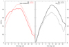 |
Fig. 16. Cross-correlation functions of the integrated Hβ line and the inner part only at ≤ ± 3000 km s−1 (left panel). CCFs based on the integrated Hα line based on SALT spectra and on additional data from the narrowband photometry (NB670 filter; see Paper I) with respect to the continuum at 4570 Å (right panel). |
3.3.2. Based on photometric light curves in combination with SALT spectra
We published the continuum data of HE 1136-2304 taken by Swift in the B band and additional B-band observations taken with the MONET North and South telescopes and with the Bochum telescopes at Cerro Armazones in Zetzl et al. (2018). Subsequently, we generated a combined B-band light curve BBochum in combination with our SALT spectral data. Furthermore, we created a combined Hα light curve Hαcomb based on the SALT spectra and the narrowband NB670 light curve taken with the Bochum telescope. In a next step we carried out some tests to ascertain whether CCFs based on various combinations of the continuum light curves and based on combined Hα light curves produce similar results.
In Table 7 we present 1) the cross-correlation lags of the spectroscopically obtained Hα light curve correlated with the combined B-band light curve and 2) the combined Hαcomb light curve correlated with the 4570 Å continuum light curve based on the SALT spectra. We also derived 3) the Hα lag from the Bochum light curves in the B and NB670 bands; the NB670 band entirely covers the broad Hα line. Because the narrowband filter contains the contribution from the AGN continuum underneath Hα in addition to Hα, we might expect two peaks in the cross correlation (see also Chelouche & Daniel 2012). To calculate the cross correlation we used the discrete correlation function (DCF; Edelson & Krolik 1988) with steps of δτ = 2 days. In comparison to the spectroscopic SALT light curves, the number of data points in this case is sufficiently high to allow for such a DCF analysis, which in general yields better results in case of unevenly sampled data. This cross correlation indeed shows two clearly distinct peaks separated by a deep minimum in between (Fig. 17). The peak at lag τ ≈ 0 days (denoted with blue dots) comes from the cross correlation of the AGN continuum in the B band with the continuum underneath the Hα line; it is virtually an autocorrelation. The second even brighter peak at τ ≈ 11 days (denoted with red dots) comes from the lag between the B-band continuum and Hα. The derived Hα lag (using the red data points) agrees within the errors with the Hα lags derived from the SALT spectra. Regarding the error limits, the derived Hα delays (11 up to 17 light days) are in good agreement with the delay of 15 light days based on the SALT spectra alone.
Cross-correlation lags of the Hα light curve with the combined B-band light curve, the combined Hα light curve with the continuum light curve based on the SALT data, and the Hα light curve based on the Bochum NB670 date with the continuum light curve based on the Bochum B-band data.
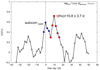 |
Fig. 17. Discrete correlation function of the Hα line based on the Bochum narrowband filter flux (NB670) with respect to the Bochum B-band flux. |
It has been demonstrated for other AGN (e.g., 3C120; Kollatschny et al. 2014) that the variability amplitude of the integrated emission lines is inversely correlated with the distance of the line-emitting regions to the central ionizing source. Figure 18 shows that this relation is valid for the broad lines in HE 1136-2304 as well. Furthermore, it has been shown that there is a radial stratification with respect to the BLR linewidths (FWHM; e.g., Kollatschny 2003). The higher ionized lines show broader linewidths (FWHM) and originate closer to the center as shown in Fig. 19. For this figure we used the corrected rotational velocities vrot as presented in Table 9 (see Sect. 3.6). For comparison with our measurements, in Fig. 19 we show the expected relations between distance and linewidth for multiple black hole masses based on the mass formula given in Sect. 3.4.
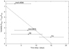 |
Fig. 18. Variability amplitude of the integrated emission lines as a function of their time delay τ (i.e., distance to the center). The dashed line indicates the linear fit to the data. |
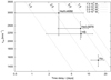 |
Fig. 19. Linewidth of the emission lines (FWHM vrot) as a function of their time delay τ (i.e., distance to the center). The dashed lines correspond to virial masses of 1.0, 2.5, 5.0, and 7.5 × 10⁷ M⊙. |
3.4. Central black hole mass
The masses of the central black holes in AGN can be estimated from the width of the broad emission line profiles, based on the assumption that the gas dynamics are dominated by the central massive object, by evaluating M = f c τcent Δv2 G−1.
It is necessary to know the distance of the line-emitting region. Characteristic distances of the individual line-emitting regions are given by the centroid τcent of the individual cross-correlation functions of the emission-line variations relative to the continuum variations (e.g., Koratkar & Gaskell 1991; Kollatschny & Dietrich 1997). The characteristic velocity Δv of the emission-line regions can be estimated from the FWHM of the rms profiles or from the line dispersions σline.
The scaling factor f in the equation above is on the order of unity and depends on the kinematics, structure, and orientation of the BLR. This scaling factor may differ from galaxy to galaxy, for example, depending on whether we see the central accretion disk including the BLR from the edge or face-on. We compared the central black hole mass value of HE 1136-2304 with values of the black hole masses derived for other AGN and adopt a mean value of f = 5.5 (e.g., Onken et al. 2004; Grier et al. 2012). This f-value might be too high by a factor of two when comparing the black hole masses with inactive galaxies (Graham et al. 2011).
Nevertheless, using f = 5.5, we calculate a mean black hole mass (see Table 8, Col. 3) of M = 3.5 ± 2.8 × 10⁷ M⊙ based on the derived delays of the integrated Balmer and Helium lines (see Table 6) and on the line dispersions σline (see Table 5). All BH masses based on the individual lines agree with each other within the error limits.
Black hole masses based on vrot, σline (rms width), and FWHM (rms width).
Using the linewidths FWHM (rms) (see Table 5) we calculated a mean black hole mass of M = 11.4 ± 9.3 × 10⁷ M⊙ (Table 8, Col. 4). However, in that case we did not correct for the contribution of turbulent motions to the width of the line profiles; this is covered in Sect. 3.6. After correcting the emission linewidths (FWHM) for their contribution of turbulent motions (Table 9, Col. 4), we derive a mean black hole mass of M = 3.8 ± 3.1 × 10⁷ M⊙ (Table 8, Col. 2). Again, all individual BH masses based on this method agree with each other within the error limits.
Line profile parameters and radius and height of the line-emitting regions for individual emission lines in HE 1136-2304.
3.5. Two-dimensional CCFs of Balmer (Hα, Hβ)and Helium I, II line profiles
We first calculated the cross-correlation lags of the integrated Balmer and Helium lines with respect to the continuum as mentioned in Sect. 3.3. Now we investigate the profile variations of these lines in more detail by calculating the lags of individual line segments. The way we proceed has been described before in our studies of line profile variations in Mrk 110 (Kollatschny & Bischoff 2002; Kollatschny 2003), Mrk 926 (Kollatschny & Zetzl 2010), and 3C120 (Kollatschny et al. 2014).
We sliced the velocity profiles of the Balmer and Helium lines into velocity segments with a width of Δv = 400 km s−1, which corresponds to the spectral resolution of our spectra. A central line segment was integrated in the velocity range −200 km s−1 ≤v≤ 200 km s−1. Afterward, we measured the intensities of all subsequent velocity segments from v = −9800 to +9800 km s−1 and compiled their light curves. Light curves of the central Balmer and Helium line segments and selected blue and red segments at 800, 2000, and 4000 km s−1 are shown in Figs. A.1–A.4. For comparison, the light curve of the continuum flux at 4570 Å is given in all these figures as well.
We computed the maximal correlation coefficient and time delay τcent of all line segment (Δv = 400 km s−1) light curves of the Balmer and Helium lines with respect to the 4570 Å continuum flux light curve. The derived time delays of the segments are shown in Figs. 20–23 as functions of distance to the line center (blue scale). The white lines in Figs. 20–23 delineate the contour lines of the correlation coefficient at different levels. The green line shows the line profile of the mean spectrum for comparison.
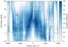 |
Fig. 20. Two-dimensional CCF(τ,v) showing the correlation coefficient of the Hα line segment light curves with the continuum light curve as a function of velocity and time delay (blue scale). Contours of the correlation coefficients are plotted at levels 0.0–0.9 every 0.05 (white lines). The green line shows the line profile of the mean spectrum. |
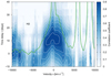 |
Fig. 21. Two-dimensional CCF(τ,v) showing the correlation coefficient of the Hβ line segment light curves with the continuum light curve as a function of velocity and time delay (blue scale). Contours of the correlation coefficients are plotted at levels 0.0–0.9 every 0.05 (white lines). The green line shows the line profile of the mean spectrum. |
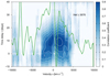 |
Fig. 22. Two-dimensional CCF(τ,v) showing the correlation coefficient of the He I λ5876 line segment light curves with the continuum light curve as functions of velocity and time delay (blue scale). Contours of the correlation coefficients are plotted at levels 0.0–0.9 every 0.05 (white lines). The green line shows the line profile of the mean spectrum. |
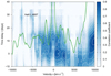 |
Fig. 23. Two-dimensional CCF(τ,v) showing the correlation coefficient of the He II λ4686 line segment light curves with the continuum light curve as functions of velocity and time delay (blue scale). Contours of the correlation coefficients are plotted at levels 0.0–0.9 every 0.05 (white lines). The green line shows the line profile of the mean spectrum. |
The following statements can be made based on these figures. There is a general trend that the Helium line response is faster than the response of the Balmer lines, as already known from the integrated lines. The velocity-delay maps are very symmetric with respect to the line center. The light curves of the emission line centers are delayed by 10–20 days with respect to the continuum variations, while the outer line wings at distances of ±2000 to ±3000 km s−1 respond much faster to continuum variations and only show a delay of 0–10 days. The delay in the outer line wings at distances of ±4000 km s−1 is even negative with respect to the optical continuum. It has been discussed in Zetzl et al. (2018) that the observed optical continuum is delayed with respect to the ionizing continuum in the UV and X-ray bands. The outer blue wing of the Hβ line shortward of −6000 km s−1) is blended with the red wing of the He II λ4686 line (see Fig. 2 as well).
3.6. Vertical BLR structure in HE 1136-2304
Information about the BLR structure in Seyfert 1 galaxies can be derived from the profiles of the broad emission lines together with variability studies (Kollatschny & Zetzl 2011, 2013a,b,c). The broad emission line profiles can be parameterized by the ratio of their full-width at half maximum (FWHM) to their line dispersion σline. We were able to show that there exists a general relation between the FWHM and the linewidth ratio FWHM/σline. The linewidth FWHM primarily reflects the line broadening of the intrinsic Lorentzian profiles due to rotational motions of the broad line gas. The intrinsic Lorentzian profiles themselves are associated with turbulent motion (see also Goad et al. 2012) and different emission lines turn out to exhibit, on average, characteristic turbulent velocities within a narrow range (Kollatschny & Zetzl 2011).
We determined the rotational velocities and turbulent velocities that belong to the individual line-emitting regions in the same way as we have done it before for other Seyfert galaxies (Kollatschny & Zetzl 2011; Kollatschny & Zetzl 2013a; Kollatschny & Zetzl 2013b; Kollatschny & Zetzl 2013c): Based on the observed linewidths (FWHM) and linewidth ratios FWHM/σline we determined the locations of the individual lines in Fig. 24. In this figure, the grid, resulting from model calculations, presents theoretical linewidth ratios based on Lorentzian profiles that are broadened owing to rotation. We read the widths of the Lorentzian profiles and the rotational velocities of the individual lines from their positions between the contour lines of constant Lorentzian linewidth and the vertical contour lines representing different vrot. The FWHM/σline versus FWHM grid based on our model calculations is publicly available1. The FWHM and FWHM/σline values we obtained for HE 1136-2304 are given in Table 9 together with the derived vturb and vrot velocities of the Balmer and Helium lines. It has been shown that the region of each emission line has a characteristic mean turbulent velocity within a narrow range (Kollatschny & Zetzl 2011, 2013a; Kollatschny et al. 2014). We derived the following mean turbulent velocities belonging to the emitting regions of the individual lines: 400 km s−1 for Hβ, 700 km s−1 for Hα, 800 km s−1 for He I λ5876, and 900 km s−1 for He II λ4686.
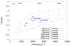 |
Fig. 24. Observed and modeled linewidth ratios FWHM/σline vs. linewidth FWHM in HE 1136-2304. The dashed curves represent the corresponding theoretical linewidth ratios based on rotational line-broadened Lorentzian profiles (FWHM = 200–3800 km s−1). The rotation velocities reach from 1000 to 5000 km s−1 (curved dotted lines from left to right). |
In the next step, we determine the heights of the line-emitting regions above the midplane as we have before for other Seyfert galaxies. The ratio of the turbulent velocity vturb with respect to the rotational velocity vrot in the line-emitting region gives us information on the ratio of the height H with respect to the radius R of the line-emitting regions as presented in Kollatschny & Zetzl (2011, 2013a), i.e.,
 (1)
(1)
The unknown viscosity parameter α is assumed to be constant and to have values of 0.1–1 (e.g., Frank et al. 2003). For simplicity we assume a value of 1 in the present investigation. The distance of the line-emitting regions of the individual lines is known from reverberation mapping (Sect. 3.3). We present in Table 9 the derived heights above the midplane of the line-emitting regions in HE 1136-2304 (in units of light days) and the ratio H/R for the individual emission lines.
The BLR structure of HE 1136-2304 is shown in Fig. 25 as a function of distance to the center and height above the midplane. The dot at radius zero gives the size of the Schwarzschild radius RS = 4.31 × 10⁻³ ld = 1.1 × 1013 cm for a black hole mass (with M = 3.8.×107 M⊙) multiplied by a factor of ten. The label on top of the figure gives the distances of the line-emitting regions in units of the Schwarzschild radius.
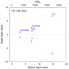 |
Fig. 25. Structure of the BLR in HE 1136-2304. The dot at radius zero has the size of a Schwarzschild black hole (for MBH = 3.8 × 10⁷ M⊙) multiplied by a factor of ten. |
As has been observed previously in other galaxies, the He II λ4686 line originates at the shortest distance from the center and the smallest height above the midplane in comparison to the Balmer and HeI lines. In comparison to Hβ, Hα originates at a larger distance from the midplane.
4. Discussion
4.1. Optical variability
We thoroughly investigated the spectroscopic variability behavior of HE 1136-2304 by taking 16 spectra over a period of six months between February to August 2015. The fractional variability Fvar was on the order of 0.1 in the optical continuum without correcting for the host galaxy flux. After correcting for the host galaxy contribution, the fractional variability Fvar of the continuum amounted to 0.25 − 0.3 (see Paper I). The integrated Balmer and Helium lines showed Fvar values of 0.1–0.5 and the higher ionized lines originating closer to the center varied with stronger amplitudes. These results describing the continuum and emission line variability are similar to those detected in other variable Seyfert galaxies such as NGC 5548 (Peterson et al. 2004), Mrk 110 (Kollatschny et al. 2001), or 3C 120 (Kollatschny et al. 2014). This confirms that the variability behavior of this changing look AGN is similar to that of other Seyfert galaxies.
4.2. Balmer decrement variability
The Balmer decrement Hα/Hβ of the narrow components has a value of 2.81. This corresponds exactly to the expected theoretical line ratio (Case B) without any reddening. However, the Balmer decrement Hα/Hβ of the broad components varies with the continuum and/or Balmer line intensity. For example, the broad line Seyfert galaxy NGC 7693 showed the same behavior based on long-term variability studies over a period of 20 years (Kollatschny et al. 2000): the Balmer decrement decreased with increasing Hβ flux.
Heard & Gaskell (2016) proposed a model with additional dust reddening clouds interior to the narrow-line region causing higher Balmer decrements in the BLR. In contrast to this model, there might be important optical depth effects in the BLR itself explaining the observations. This is consistent with the finding that Hα originates at twice the distance of Hβ. A similar radial stratification as seen in HE 1136-2304 has been observed in, for example, Arp 151 (Bentz et al. 2010) as well. It has been discussed by Korista (2004) that the radial stratification is a result of optical-depth effects of the Balmer lines: the broad-line Balmer decrement decreases in high continuum states and steepens in low states exactly as observed in HE 1136-2304 (see Fig. 4). The continuum varied by a factor of nearly two during our campaign in 2015. However, we did not detect simultaneous variations of the Seyfert subtype during our observing period of seven months. A variation of Seyfert subtypes might be connected with stronger continuum amplitudes and/or longer timescales as has been seen before, for example, in Fairall 9 (Kollatschny & Fricke 1985).
4.3. Hβ lag versus optical continuum luminosity
Now we want to test whether HE 1136-2304 follows the general trend in the radius-luminosity relationship for AGN (Kaspi et al. 2000; Bentz et al. 2013). We determined a continuum luminosity logλLλ of 42.6054 erg s−1 (0.47 × 10⁻¹⁵ erg s−1 cm−2 Å−1) in the optical at 5100 Å after correction for the contribution of the host galaxy (Zetzl et al. 2018). Furthermore, we derived a mean radius of 7.5 light days for the Hβ line-emitting region based on the delay of the integrated Hβ line variability curve with respect to the optical continuum light curve.
Figure 26 shows the optical continuum luminosity and Hβ-optical lags for HE 1136-2304 (red), for NGC 5548 based on different variability campaigns (black; Pei et al. 2017 based on Kilerci Eser et al. 2015; Denney et al. 2009), and a sample of other AGN excluding NGC 5548 (green; Bentz et al. 2013). The black line is the linear least-squares fit to the NGC 5548 data as presented by Pei et al. (2017). The R − L(5100 Å) relationship is given by
![Mathematical equation: $$ \begin{aligned} \log \left[\frac{R_{\rm BLR}}{ 1\,\mathrm{light-day}}\right] = K +\beta \log \left[\frac{\lambda L_{\lambda }(5100\,\AA )}{{10^{44}\, \mathrm{erg\,s }}^{-1}}\right], \end{aligned} $$](/articles/aa/full_html/2018/11/aa33727-18/aa33727-18-eq29.gif) (2)
(2)
where K is the origin and β is the slope. The red solid line gives the best-fit linear regression to the whole AGN sample. The data of HE 1136-2304 is in very good accordance with the general Hβ lag versus the optical continuum luminosity relation.
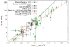 |
Fig. 26. Optical continuum luminosity and Hβ-optical lags for HE 1136-2304 and other AGN. |
The red solid line has a slope β of 0.53, which is therefore identical to the best-fit slope of  of Bentz et al. (2013). This value is very close to the value of 0.5 expected from simple photoionization arguments, i.e.,
 (3)
(3)
(e.g., Kaspi et al. 2000; Bentz et al. 2013; and references therein).
We tested whether the β slope approaches values even closer to 0.5 or whether the Pearson correlation coefficient becomes higher if we add a few light days to the Hβ radius. Such an additional delay might be caused by the fact that the optical continuum is generally delayed by a few light days with respect to the driving X-ray light curve (Zetzl et al. 2018; Shappee et al. 2014; Fausnaugh et al. 2016).
We added additional lags of one to eight light days to all Hβ-optical lags to take into account a systematic delay of the optical bands with respect to the driving X-ray flux. A time delay of eight light days is an upper limit based on the correlation of the optical band light curves with respect to the XRT light curve (Zetzl et al. 2018). Figures 27 and 28 show the Hβ lag versus optical continuum luminosity diagrams with an additional lag of one and four days, respectively, taking into account the optical-X-ray lag.
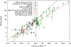 |
Fig. 27. Optical continuum luminosity and Hβ-optical lags for HE 1136-2304 and other AGN (plus 1 day additional lag for optical-X-ray lag). |
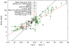 |
Fig. 28. Optical continuum luminosity and Hβ-optical lags for HE 1136-2304 and other AGN (plus 4 days additional lag for optical-X-ray lag). |
Table 10 gives the Pearson correlation coefficient for the relation between optical continuum luminosities and Hβ-optical lags. The Hβ lags have been modified assuming additional lags (in units of days) for the optical lag with respect to the driving X-ray source. Furthermore, we present the β values for the additional delays that have been assumed. We get the highest correlation coefficient for an additional delay of four days. We reached a β slope of exactly 0.5 for an additional delay of one day.
Pearson correlation coefficient for the relation between optical continuum luminosities and Hβ-optical lags.
4.4. Structure and kinematics in the BLR
4.4.1. Mean and rms line profiles
The mean and rms line profiles of the broad emission lines give us information about the kinematics and structure of the line-emitting BLR region. Differences in the broad-line widths of the rms and mean profiles (see Figs. 6–8) might be caused by a radial stratification of optical depth effects in these lines (Korista 2004). Especially the rms profiles of the Balmer lines in HE 1136-2304 show an asymmetric triple structure. Aside from a central component there were additional blue and red components at ±1400 km s−1 (see Fig. 13). These components are barely visible in the mean profiles. The additional component in the red wing is by far stronger than that in the blue wing. An additional weak blue component, which is nearly symmetrical to the red component, is apparent in the rms profile of Hβ (Fig. 13). Furthermore, this red rms component varies relatively stronger in the Hβ line than in Hα. The additional blue and red components in the line profiles – in addition to the central component – are an indication that the line-emitting region is connected to the accretion disk. Such double-peaked profiles are considered to be ubiquitous signatures of accretion disks (e.g., Eracleous & Halpern 2003; Gezari et al. 2007; Shapovalova et al. 2013; Storchi-Bergmann et al. 2017; and references therein). In some cases these double-peaked profiles become only visible in the rms line profiles as in NGC 4593, for example (Kollatschny & Dietrich 1997). The variable Seyfert galaxy Akn 120 is another example of a very strong red component showing up in the Hβ wing within one year (Kollatschny et al. 1981).
Similar to the line profiles in NGC 4593 (Kollatschny & Dietrich 1997), the rms line profiles of Hα and Hβ in HE 1136-2304 show a steeper red wing and a flatter outer blue wing indicating an additional outflow component (see Fig. 13). The outer blue wing is even more pronounced in the higher ionized Helium lines in comparison to the Balmer lines (see Fig. 14), indicating a stronger outflow in the inner BLR.
4.4.2. Velocity delay maps
The 2D-CCFs or velocity-delay maps shown in Figs. 20–23 contain additional information about the structure and kinematics of the BLR. We compare the derived velocity delay maps of HE 1136-2304 with theoretical models for the structure and kinematics of the BLR (Welsh & Horne 1991; Horne et al. 2004; Goad et al. 2012; Grier et al. 2013) and with velocity delay maps of other AGN. All the velocity delay maps are very symmetric with respect to their line centers at v = 0 km s−1. The delays in the wings are by far shorter than in the line center. Such behavior is typical for thin Keplerian disk BLR models (Welsh & Horne 1991; Horne et al. 2004; Grier et al. 2013). There is an indication in the velocity delay maps of the Balmer lines that the response in the red wing (at v = 3000 − 5000 km s−1) is slightly stronger and that it shows a shorter delay than in the blue wing. This might be caused by an additional inflow component (Welsh & Horne 1991), by hydro-magnetically driven wind (Horne et al. 2004), or by an additional turbulent component (Goad et al. 2012).
The velocity delay maps of other Seyfert galaxies in general show two different trends: a more symmetrical velocity delay map that is typical for Keplerian disks or a velocity delay map showing a strong red component caused by strong inflow or hydro-magnetically driven wind, and a combination of both. NGC 4593 (Kollatschny & Dietrich 1997), 3C 120 (Kollatschny et al. 2014), Mrk 50 (Barth et al. 2011), and NGC 5548 (Pei et al. 2017; and references therein) show a more symmetrical velocity delay map. NGC 3516 (Denney et al. 2010), Mrk1501, PG 2130+099 (Grier et al. 2013) and Mrk 335 (Du et al. 2016) show a dominant red component. Velocity delay maps of other galaxies indicate a combination of dominant Keplerian motion and an additional red component, such as Mrk 110 (Kollatschny et al. 2001) and Arp 151 (Bentz et al. 2010). However, there are three exceptions (Mrk 817, NGC 3227, and Mrk 142) in which only a strong blue component is present in the velocity delay maps (Denney et al. 2010; Du et al. 2016). The velocity delay map of the changing look AGN HE 1136-2304 is similar to that of most other AGN. It shows a dominant Keplerian motion component with a slightly more intense red component.
4.5. Vertical BLR structure in a sample of AGN
The higher ionized broad emission lines originate at smaller radii as shown in Sect. 3.3. Furthermore, the integrated Hα originates at a distance of 15 light days and therefore at twice the distance of Hβ (see Table 6). Moreover, it has been shown that the higher ionized lines originate closer to the midplane of the accretion disk in comparison to the lower ionized lines. We presented the BLR structure as a function of distance to the center and height above the midplane (Fig. 25). The He II λ4686 line originates closest to the midplane. Hα originates at a larger distance from the midplane in comparison to Hβ. Such a trend has been observed before in other galaxies as NGC 7469 (Kollatschny & Zetzl 2013c) and 3C 120 (Kollatschny et al. 2014).
A second trend has been found when comparing the Hβ distances above the midplane for different active galaxies: galaxies showing the broadest Hβ linewidths originate closest to the midplane, while galaxies showing the narrowest Hβ linewidths originate at the largest distance to the midplane (Kollatschny et al. 2014). The linewidths (with respect to the individual lines) are therefore a characteristic for the height of the line-emitting regions above the midplane. We present the height-to-radius ratio and FWHM of Hβ for a sample of AGN (Kollatschny et al. 2014) and for HE 1136-2304 in Table 11. The height-to-radius ratio for Hβ is largest for galaxies showing narrow emission lines and smallest for galaxies with broad lines. The overall picture we derived for the BLR region structure previously in Kollatschny & Zetzl (2013c) and Kollatschny et al. (2014) is confirmed by the additional emission line data of HE 1136-2304. The derived height-to-radius ratio for HE 1136-2304 confirms the general trend (see Fig. 29). Again, the HE 1136-2304 data support the picture that the broad emission line geometries of AGN are not simply scaled-up versions depending only on the central luminosity (and central black hole mass).
Height-to-radius ratio and FWHM of Hβ for a sample of AGN.
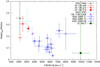 |
Fig. 29. Height-to-radius ratio for the Hβ line-emitting regions for a sample of AGN showing different Hβ linewidths (FWHM). |
5. Summary
We present results of a spectral monitoring campaign of the changing look AGN HE 1136-2304 obtained by the 10 m SALT telescope between 2014 December and 2015 July. These observations were taken subsequently to a continuum outburst detected in the X-rays and in the optical in 2014 July. Our findings can be summarized as follows:
-
(1)
The BLR in HE 1136-2304 is stratified with respect to the distance of the individual line-emitting regions. The integrated emission line intensities of Hα, Hβ, He I λ5876, and He II λ4686 originate at distances of
 ,
,  ,
,  , and
, and  light days with respect to the optical continuum at 4570 Å. The variability amplitudes of the integrated emission lines are a function of distance to the ionizing source as well.
 -
(2)
We derived a central black hole mass of 3.8 × 10⁷ M⊙ based on the linewidths, corrected for the turbulent component, and distances of the line-emitting regions.
-
(3)
Based on velocity delay maps, the light curves of the emission line centers are delayed by 10–20 days with respect to the continuum variations. The outer line wings of the emission lines respond much faster to the continuum variations in all lines indicating an Keplerian disk component for the broad line-emitting region. The response in the outer wings is even shorter than the response of the adjacent optical continuum flux with respect to the ionizing continuum flux by about two light days.
-
(4)
The vertical BLR structure in HE 1136-2304 confirms the general trend that line emitting regions in AGN showing narrower emission lines originate at larger distances from the midplane in comparison to AGN showing broader emission lines.
-
(5)
In general, the variability behavior of the changing look AGN HE 1136-2304 is similar to that of other AGN.
Acknowledgments
This work has been supported by the DFG grants Ko 857/33-1 and Ha3555/12-2.
References
- Barth, A. J., Pancoast, A., Thorman, S. J., et al. 2011, ApJ, 743, L4 [NASA ADS] [CrossRef] [Google Scholar]
- Bentz, M. C., Horne, K., Barth, A. J., et al. 2010, ApJ, 720, L46 [NASA ADS] [CrossRef] [Google Scholar]
- Bentz, M. C., Denney, K. D., Grier, C. J., et al. 2013, ApJ, 767, 149 [NASA ADS] [CrossRef] [Google Scholar]
- Chelouche, D., & Daniel, E. 2012, ApJ, 747, 62 [NASA ADS] [CrossRef] [Google Scholar]
- Collin-Souffrin, S., Alloin, D., & Andrillat, Y. 1973, A&A, 22, 343 [NASA ADS] [Google Scholar]
- Dietrich, M., & Kollatschny, W. 1995, A&A, 303, 405 [NASA ADS] [Google Scholar]
- Denney, K. D., Peterson, B. M., Pogge, R. W., et al. 2009, ApJ, 704, L80 [NASA ADS] [CrossRef] [Google Scholar]
- Denney, K. D., Peterson, B. M., Pogge, R. W., et al. 2010, ApJ, 721, 715 [NASA ADS] [CrossRef] [Google Scholar]
- Denney, K. D., De Rosa, G., Croxall, K., et al. 2014, ApJ, 796, 134 [NASA ADS] [CrossRef] [Google Scholar]
- Du, P., Lu, K. X., Hu, C., et al. 2016, ApJ, 820, 27 [NASA ADS] [CrossRef] [Google Scholar]
- Edelson, R., & Krolik, J. 1988, ApJ, 333, 646 [NASA ADS] [CrossRef] [Google Scholar]
- Edelson, R., Gelbord, J. M., Horne, K., et al. 2015, ApJ, 806, 129 [NASA ADS] [CrossRef] [Google Scholar]
- Eracleous, M., & Halpern, J. 2003, ApJ, 599, 886 [NASA ADS] [CrossRef] [Google Scholar]
- Fausnaugh, M. M., Denney, K. D., Barth, A. J., et al. 2016, ApJ, 821, 56 [NASA ADS] [CrossRef] [Google Scholar]
- Frank, J., King, A., & Raine, D. 2003, Accretion Power in Astrophysics (Cambridge University Press) [Google Scholar]
- Fromerth, M. J., & Melia, F. 2000, ApJ, 533, 172 [NASA ADS] [CrossRef] [Google Scholar]
- Gaskell, C. M. 2009, New Astron. Rev., 53, 114 [Google Scholar]
- Gaskell, C. M., & Peterson, B. M. 1987, ApJS, 65, 1 [NASA ADS] [CrossRef] [Google Scholar]
- Gezari, S., Halpern, J. P., & Eracleous, M. 2007, ApJS, 169, 167 [NASA ADS] [CrossRef] [Google Scholar]
- Goad, M. R., Korista, K. T., & Ruff, A. J. 2012, MNRAS, 426, 3086 [NASA ADS] [CrossRef] [Google Scholar]
- Graham, A. W., Onken, C. A., Athanassoula, E., & Combes, F. 2011, MNRAS, 412, 2211 [NASA ADS] [CrossRef] [Google Scholar]
- Grier, C. J., Peterson, B. M., Pogge, R. W., et al. 2012, ApJ, 755, 60 [NASA ADS] [CrossRef] [Google Scholar]
- Grier, C. J., Peterson, B. M., Horne, K., et al. 2013, ApJ, 764, 47 [NASA ADS] [CrossRef] [Google Scholar]
- Heard, C. Z., & Gaskell, C. M. 2016, MNRAS, 461, 4227 [NASA ADS] [CrossRef] [Google Scholar]
- Horne, K., Peterson, B. M., Collier, S. J., & Netzer, H. 2004, PASP, 116, 465 [NASA ADS] [CrossRef] [Google Scholar]
- Kaspi, S., Smith, P. S., Netzer, H., et al. 2000, ApJ, 533, 631 [NASA ADS] [CrossRef] [Google Scholar]
- Kilerci Eser, E., Vestergaard, M., Peterson, B. M., Denney, K. D., & Bentz, M. C. 2015, ApJ, 801, 8 [NASA ADS] [CrossRef] [Google Scholar]
- Kollatschny, W. 2003, A&A, 407, 461 [NASA ADS] [CrossRef] [EDP Sciences] [Google Scholar]
- Kollatschny, W., & Bischoff, K. 2002, A&A, 386, L19 [NASA ADS] [CrossRef] [EDP Sciences] [Google Scholar]
- Kollatschny, W., & Dietrich, M. 1996, A&A, 314, 43 [NASA ADS] [Google Scholar]
- Kollatschny, W., & Dietrich, M. 1997, A&A, 323, 5 [NASA ADS] [Google Scholar]
- Kollatschny, W., & Fricke, K. J. 1985, A&A, 146, L11 [NASA ADS] [Google Scholar]
- Kollatschny, W., & Zetzl, M. 2010, A&A, 522, A36 [NASA ADS] [CrossRef] [EDP Sciences] [Google Scholar]
- Kollatschny, W., & Zetzl, M. 2011, Nature, 470, 366 [NASA ADS] [CrossRef] [Google Scholar]
- Kollatschny, W., & Zetzl, M. 2013a, A&A, 549, A100 [NASA ADS] [CrossRef] [EDP Sciences] [Google Scholar]
- Kollatschny, W., & Zetzl, M. 2013b, A&A, 551, L6 [NASA ADS] [CrossRef] [EDP Sciences] [Google Scholar]
- Kollatschny, W., & Zetzl, M. 2013c, A&A, 558, A26 [NASA ADS] [CrossRef] [EDP Sciences] [Google Scholar]
- Kollatschny, W., Fricke, K. J., Schleicher, H., & Yorke, H. W. 1981, A&A, 102, L23 [NASA ADS] [Google Scholar]
- Kollatschny, W., Bischoff, K., & Dietrich, M. 2000, A&A, 361, 901 [NASA ADS] [Google Scholar]
- Kollatschny, W., Bischoff, K., Robinson, E. L., Welsh, W. F., & Hill, G. J. 2001, A&A, 379, 125 [NASA ADS] [CrossRef] [EDP Sciences] [Google Scholar]
- Kollatschny, W., Ulbrich, K., Zetzl, M., Kaspi, S., & Haas, M. 2014, A&A, 566, A106 [NASA ADS] [CrossRef] [EDP Sciences] [Google Scholar]
- Komossa, S., Zhou, H., Wang, T., et al. 2008, ApJ, 678, L13 [NASA ADS] [CrossRef] [Google Scholar]
- Koratkar, A. P., & Gaskell, M. 1991, ApJ, 370, L61 [NASA ADS] [CrossRef] [Google Scholar]
- Korista, K. T., & Goad, M. R. 2004, ApJ, 606, 749 [NASA ADS] [CrossRef] [Google Scholar]
- LaMassa, S. M., Cales, S., Moran, E. C., et al. 2015, ApJ, 800, 144 [NASA ADS] [CrossRef] [Google Scholar]
- MacLeod, C. L., Ross, N. P., Lawrence, A., et al. 2016, MNRAS, 457, 389 [NASA ADS] [CrossRef] [Google Scholar]
- Onken, C. A., Ferrarese, L., Merritt, D., et al. 2004, ApJ, 615, 645 [NASA ADS] [CrossRef] [Google Scholar]
- Osterbrock, D. E. 1981, ApJ, 249, 462 [NASA ADS] [CrossRef] [Google Scholar]
- Parker, M. L., Komossa, S., Kollatschny, W., et al. 2016, MNRAS, 461, 1927 [NASA ADS] [CrossRef] [Google Scholar]
- Pei, L., Fausnaugh, M. M., Barth, A. J., et al. 2017, ApJ, 837, 131 [NASA ADS] [CrossRef] [Google Scholar]
- Penston, M. V., & Perez, E. 1984, MNRAS, 211, 33 [Google Scholar]
- Peterson, B. M., Wanders, I., Bertram, R., et al. 1998, ApJ, 501, 82 [NASA ADS] [CrossRef] [Google Scholar]
- Peterson, B. M., Berlind, P., Bertram, R., et al. 2002, ApJ, 581, 197 [NASA ADS] [CrossRef] [Google Scholar]
- Peterson, B. M., Ferrarese, L., Gilbert, K. M., et al. 2004, ApJ, 613, 682 [NASA ADS] [CrossRef] [Google Scholar]
- Runnoe, J. C., Cales, S., Ruan, J. J., et al. 2016, MNRAS, 455, 1691 [NASA ADS] [CrossRef] [Google Scholar]
- Shapovalova, A. I., Popović, L. \’{C}., Burenkov, A. N., et al. 2010, A&A, 517, A42 [NASA ADS] [CrossRef] [EDP Sciences] [Google Scholar]
- Shapovalova, A. I., Popović, L. \’{C}., Burenkov, A. N., et al. 2013, A&A, 559, A10 [NASA ADS] [CrossRef] [EDP Sciences] [Google Scholar]
- Shappee, B. J., Prieto, J. L., Grupe, D., et al. 2014, ApJ, 788, 48 [NASA ADS] [CrossRef] [Google Scholar]
- Storchi-Bergmann, T., Nemmen da Silva, R., Eracleous, M., et al. 2003, ApJ, 598, 956 [NASA ADS] [CrossRef] [Google Scholar]
- Storchi-Bergmann, T., Schimoia, J. S., Peterson, B. M., et al. 2017, ApJ, 835, 236 [NASA ADS] [CrossRef] [Google Scholar]
- Reimers, D., Koehler, T., & Wisotzki, L. 1996, A&AS, 115, 235 [NASA ADS] [Google Scholar]
- Welsh, W. F., & Horne, K. 1991, ApJ, 379, 586 [NASA ADS] [CrossRef] [Google Scholar]
- Wright, E. L. 2006, PASP, 118, 1711 [NASA ADS] [CrossRef] [Google Scholar]
- Zetzl, M., Kollatschny, W., & Ochmann, M. W. 2018, A&A, 618, A83 (Paper I) [NASA ADS] [CrossRef] [EDP Sciences] [Google Scholar]
Appendix A: Additional figures
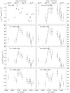 |
Fig. A.1. Light curves of the continuum flux at 4570 Å and of selected Hα line segments (in units of 10−15 erg s−1 cm−2): Hαcenter and segments at v = ±800, ±2000, ±4000 km s−1. |
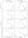 |
Fig. A.2. Light curves of the continuum flux at 4570 Å and of selected Hβ line segments (in units of 10−15 erg s−1 cm−2): Hβcenter and segments at v = ±800, ±2000, ±4000 km s−1. |
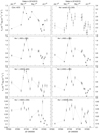 |
Fig. A.3. Light curves of the continuum flux at 4570 Å and of selected He I λ5876 line segments (in units of 10−15 erg s−1 cm−2): He I λ5876center and segments at v = ±800, ±2000, ±4000 km s−1. |
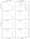 |
Fig. A.4. Light curves of the continuum flux at 4570 Å and of selected He II λ4686 line segments (in units of 10−15 erg s−1 cm−2): He II λ4686center and segments at v = ±800, ±2000, ±4000 km s−1. |
All Tables
Variability statistics based on the SALT data in units of 10−15 erg s−1 cm−2 Å−1 for the continuum as well as in units of 10−15 erg s−1 cm−2 for the emission lines.
Balmer and Helium linewidths: FWHM of the mean and rms line profiles as well as the line dispersion σline of the rms profiles.
Cross-correlation lags of the Balmer and Helium line light curves with respect to the 4570 Å continuum light curve.
Cross-correlation lags of the Hα light curve with the combined B-band light curve, the combined Hα light curve with the continuum light curve based on the SALT data, and the Hα light curve based on the Bochum NB670 date with the continuum light curve based on the Bochum B-band data.
Line profile parameters and radius and height of the line-emitting regions for individual emission lines in HE 1136-2304.
Pearson correlation coefficient for the relation between optical continuum luminosities and Hβ-optical lags.
All Figures
|
Fig. 1. Optical spectra of HE 1136-2304 taken with the SALT telescope for our variability campaign from December 2014 until July 2015. |
| In the text | |
|
Fig. 2. Integrated mean (black) and rms (red) spectra for our variability campaign of HE 1136-2304. The rms spectrum has been scaled by a factor of 6.9 to enhance weak line structures. |
| In the text | |
|
Fig. 3. Light curves of the continuum fluxes at 4570 Å and 5360 Å (in units of 10−15 erg cm−2 s−1 Å−1) as well as of the integrated emission line fluxes of Hα, Hβ, He II λ4686, and He I λ5876 (in units of 10−14 erg cm−2 s−1) for our variability campaign from 2014 December until 2015 July. |
| In the text | |
|
Fig. 4. Balmer decrement Hα/Hβ of the broad line components vs. the continuum intensity at 4570 Å. The dashed line on the graph represents the linear regression. |
| In the text | |
|
Fig. 5. Balmer decrement Hα/Hβ of the broad line components vs. broad line Hβ intensity. The dashed line on the graph represents the linear regression. |
| In the text | |
|
Fig. 6. Normalized mean (blue), mean without a narrow component (black), and rms (red) line profiles of Hα in velocity space. |
| In the text | |
|
Fig. 7. Normalized mean (blue), mean without a narrow component (black), and rms (red) line profiles of Hβ in velocity space. |
| In the text | |
|
Fig. 8. Normalized mean (blue), mean without a narrow component (black), and rms (red) line profiles of He I λ5876 in velocity space. |
| In the text | |
|
Fig. 9. Normalized mean (blue), mean without a narrow component (black), and rms (red) line profiles of He II λ4686 in velocity space. |
| In the text | |
|
Fig. 10. Normalized mean line profiles of Hα, Hβ, He I λ5876, and He II λ4686. |
| In the text | |
|
Fig. 11. Normalized mean line profiles of Hα, Hβ without a narrow component. In addition, we flipped the profiles at v = 0 km s−1. |
| In the text | |
|
Fig. 12. Normalized mean line profiles of Hβ, He I λ5876, and He II λ4686 without a narrow component. |
| In the text | |
|
Fig. 13. Normalized rms line profiles of Hα, Hβ. In addition, we flipped the profiles at v = 0 km s−1. |
| In the text | |
|
Fig. 14. Normalized rms line profiles of Hβ, He I λ5876, and He II λ4686. |
| In the text | |
|
Fig. 15. Cross-correlation functions of the integrated Hα, Hβ, He I λ5876, and He II λ4686 lines with respect to the continuum at 4570 Å. |
| In the text | |
|
Fig. 16. Cross-correlation functions of the integrated Hβ line and the inner part only at ≤ ± 3000 km s−1 (left panel). CCFs based on the integrated Hα line based on SALT spectra and on additional data from the narrowband photometry (NB670 filter; see Paper I) with respect to the continuum at 4570 Å (right panel). |
| In the text | |
|
Fig. 17. Discrete correlation function of the Hα line based on the Bochum narrowband filter flux (NB670) with respect to the Bochum B-band flux. |
| In the text | |
|
Fig. 18. Variability amplitude of the integrated emission lines as a function of their time delay τ (i.e., distance to the center). The dashed line indicates the linear fit to the data. |
| In the text | |
|
Fig. 19. Linewidth of the emission lines (FWHM vrot) as a function of their time delay τ (i.e., distance to the center). The dashed lines correspond to virial masses of 1.0, 2.5, 5.0, and 7.5 × 10⁷ M⊙. |
| In the text | |
|
Fig. 20. Two-dimensional CCF(τ,v) showing the correlation coefficient of the Hα line segment light curves with the continuum light curve as a function of velocity and time delay (blue scale). Contours of the correlation coefficients are plotted at levels 0.0–0.9 every 0.05 (white lines). The green line shows the line profile of the mean spectrum. |
| In the text | |
|
Fig. 21. Two-dimensional CCF(τ,v) showing the correlation coefficient of the Hβ line segment light curves with the continuum light curve as a function of velocity and time delay (blue scale). Contours of the correlation coefficients are plotted at levels 0.0–0.9 every 0.05 (white lines). The green line shows the line profile of the mean spectrum. |
| In the text | |
|
Fig. 22. Two-dimensional CCF(τ,v) showing the correlation coefficient of the He I λ5876 line segment light curves with the continuum light curve as functions of velocity and time delay (blue scale). Contours of the correlation coefficients are plotted at levels 0.0–0.9 every 0.05 (white lines). The green line shows the line profile of the mean spectrum. |
| In the text | |
|
Fig. 23. Two-dimensional CCF(τ,v) showing the correlation coefficient of the He II λ4686 line segment light curves with the continuum light curve as functions of velocity and time delay (blue scale). Contours of the correlation coefficients are plotted at levels 0.0–0.9 every 0.05 (white lines). The green line shows the line profile of the mean spectrum. |
| In the text | |
|
Fig. 24. Observed and modeled linewidth ratios FWHM/σline vs. linewidth FWHM in HE 1136-2304. The dashed curves represent the corresponding theoretical linewidth ratios based on rotational line-broadened Lorentzian profiles (FWHM = 200–3800 km s−1). The rotation velocities reach from 1000 to 5000 km s−1 (curved dotted lines from left to right). |
| In the text | |
|
Fig. 25. Structure of the BLR in HE 1136-2304. The dot at radius zero has the size of a Schwarzschild black hole (for MBH = 3.8 × 10⁷ M⊙) multiplied by a factor of ten. |
| In the text | |
|
Fig. 26. Optical continuum luminosity and Hβ-optical lags for HE 1136-2304 and other AGN. |
| In the text | |
|
Fig. 27. Optical continuum luminosity and Hβ-optical lags for HE 1136-2304 and other AGN (plus 1 day additional lag for optical-X-ray lag). |
| In the text | |
|
Fig. 28. Optical continuum luminosity and Hβ-optical lags for HE 1136-2304 and other AGN (plus 4 days additional lag for optical-X-ray lag). |
| In the text | |
|
Fig. 29. Height-to-radius ratio for the Hβ line-emitting regions for a sample of AGN showing different Hβ linewidths (FWHM). |
| In the text | |
|
Fig. A.1. Light curves of the continuum flux at 4570 Å and of selected Hα line segments (in units of 10−15 erg s−1 cm−2): Hαcenter and segments at v = ±800, ±2000, ±4000 km s−1. |
| In the text | |
|
Fig. A.2. Light curves of the continuum flux at 4570 Å and of selected Hβ line segments (in units of 10−15 erg s−1 cm−2): Hβcenter and segments at v = ±800, ±2000, ±4000 km s−1. |
| In the text | |
|
Fig. A.3. Light curves of the continuum flux at 4570 Å and of selected He I λ5876 line segments (in units of 10−15 erg s−1 cm−2): He I λ5876center and segments at v = ±800, ±2000, ±4000 km s−1. |
| In the text | |
|
Fig. A.4. Light curves of the continuum flux at 4570 Å and of selected He II λ4686 line segments (in units of 10−15 erg s−1 cm−2): He II λ4686center and segments at v = ±800, ±2000, ±4000 km s−1. |
| In the text | |
Current usage metrics show cumulative count of Article Views (full-text article views including HTML views, PDF and ePub downloads, according to the available data) and Abstracts Views on Vision4Press platform.
Data correspond to usage on the plateform after 2015. The current usage metrics is available 48-96 hours after online publication and is updated daily on week days.
Initial download of the metrics may take a while.