| Issue |
A&A
Volume 619, November 2018
|
|
|---|---|---|
| Article Number | A25 | |
| Number of page(s) | 12 | |
| Section | The Sun | |
| DOI | https://doi.org/10.1051/0004-6361/201833058 | |
| Published online | 01 November 2018 | |
Measuring the electron temperatures of coronal mass ejections with future space-based multi-channel coronagraphs: a numerical test
1 INAF – Turin Astrophysical Observatory, via Osservatorio 20, 10025 Pino Torinese (TO), Italy
e-mail: This email address is being protected from spambots. You need JavaScript enabled to view it.
2 School of Mathematics and Statistics, University of St. Andrews, North Haugh, St. Andrews, Fife KY16 9SS, UK
Received:
20
March
2018
Accepted:
13
July
2018
Abstract
Context. The determination from coronagraphic observations of physical parameters of the plasma embedded in coronal mass ejections (CMEs) is of crucial importance for our understanding of the origin and evolution of these phenomena.
Aims. The aim of this work is to perform the first ever numerical simulations of a CME as it will be observed by future two-channel (visible light VL and UV Ly-α) coronagraphs, such as the Metis instrument on-board ESA-Solar Orbiter mission, or any other future coronagraphs with the same spectral band-passes. These simulations are then used to test and optimize the plasma diagnostic techniques to be applied to future observations of CMEs.
Methods. The CME diagnostic techniques are tested here by analyzing synthetic coronagraphic observations. First, a numerical three-dimensional (3D) magnetohydrodynamic (MHD) simulation of a CME is performed, and the plasma parameters in the simulation are used to generate synthetic visible light (VL) and ultraviolet (UV) coronagraphic two-dimensional (2D) images of the eruption (i.e., integrated along the line-of-sight). Second, synthetic data are analyzed with different assumptions (as will be done with real data), to infer the kinematic properties of the CME (such as the extension along the line-of-sight of the emitting region, the expansion speed, and the CME propagation direction), as well as physical parameters of the CME plasma (the plasma electron density and temperature). A comparison between input parameters from the simulation and output parameters from the synthetic data analysis is then performed.
Results. The inversion of VL polarized data allows to successfully determine the CME speed and 3D propagation direction (with the polarization ratio technique), as well as to derive information on the extension along the line-of-sight of the emitting plasma, a crucial parameter needed to convert the plasma electron column densities into number densities. These parameters are used to analyze UV Ly-α images and to estimate the CME plasma temperature, also taking into account Doppler dimming effect. Output plasma temperatures are in general underestimated, both in the CME body and core regions. By neglecting the UV Ly-α radiative excitation of H atoms, reliable temperatures can be more easily derived in the CME core (within ∼60%). On the other hand, we show that a determination of temperatures (within ∼20−30%) in the CME body requires 2D maps of CME radial speeds and Doppler dimming coefficients to be derived.
Key words: Sun: coronal mass ejections (CMEs) / Sun: UV radiation / methods: numerical / methods: data analysis / plasmas
© ESO 2018
1. Introduction
The availability of space-based coronagraphs and heliospheric imagers on-board SOHO and STEREO spacecraft over the last two decades permitted continuous observations of coronal mass ejections (CMEs), providing an unprecedented view of these and other dynamic phenomena occurring in the solar corona (see review by Webb & Howard 2012). The visible light (VL) imaging of CMEs allowed many authors to study the details of many CME properties, such as their kinematics, masses, external forces acting during their propagation, three-dimensional (3D) structure, and CME-driven shocks (see e.g., Bemporad & Mancuso 2010; Colaninno & Vourlidas 2009; Gopalswamy & Yashiro 2011; Ontiveros & Vourlidas 2009, Michałek et al. 2003; Mierla et al. 2010; Rouillard et al. 2011; Thernisien et al. 2009; Yashiro et al. 2004; Zhang et al. 2004). Moreover, the availability of a large amount of data provided an opportunity to study CMEs and their relationships (from a statistical point of view) to other phenomena such as solar flares, solar energetic particles (SEPs), prominences and filaments, and solar radio bursts, covering almost entirely two solar activity cycles (see e.g., Dierckxsens et al. 2015; Gilbert et al. 2000; Gopalswamy et al. 2002; Nindos et al. 2008; Reames 2013; Temmer et al. 2010; Vourlidas et al. 2013). Space-based coronagraph instruments also demonstrate their unique capabilities to continuously monitor the inner and intermediate atmosphere of the Sun (typically for altitudes between ∼1 and ∼30 R⊙), and to provide fundamental boundary conditions required to forecast the possible impact of CMEs on Earth, thus demonstrating their leading role in space weather applications (see e.g., Kim et al. 2005; Michalek et al. 2007; Schwenn et al. 2005).
Beside the significant discoveries provided by VL coronagraphs, an impressive amount of new results has been released thanks to the UltraViolet (UV) Coronagraph Spectrometer (UVCS; Kohl et al. 1995) on-board SOHO. The UVCS instrument provided the first ever continuous observations of the UV spectroscopic emission by CMEs during their early expansion phases in the inner corona (typically for altitudes between ∼0.5 and ∼5 R⊙). When the eruptions crossed the spectrometer field of view, these observations allowed to derive detailed information on many CME plasma parameters that cannot be derived from VL coronagraphy alone, such as plasma proton and electron temperatures, heavy ion kinetic temperatures, and elemental distributions (Akmal et al. 2001; Bemporad et al. 2007; Ciaravella et al. 2003, 2006; Raymond et al. 2003; Susino & Bemporad 2016). Hundreds of CMEs have been observed by UVCS (see review by Kohl et al. 2006), and the most prominent events observed during the first 10 years of the SOHO mission have been classified in the UVCS CME catalog1, and integrated with the LASCO CME CDAW catalog (Giordano et al. 2013). Recently it was also shown for the first time that UVCS observations of CMEs can be integrated with STEREO observations to complement spectroscopy with stereoscopy, and that the combination of VL and UV coronography can provide a unique description of plasma across CME-driven shocks (Susino et al. 2014). Moreover, UVCS also observed the eruption of many erupting prominences embedded in CMEs, and the analysis of the available data is still on-going (e.g., Jejčič et al. 2017; Heinzel et al. 2016).
Despite the importance of the space-based coronagraphy for science on CMEs briefly outlined above, as well as its Space Weather applications, only a few similar instruments will be launched by space agencies over the next decade. In particular, one of them will be Metis (Romoli et al. 2017; Antonucci et al. 2012; Fineschi et al. 2012) on board the ESA-Solar Orbiter mission (Müller & Marsden 2013), to be launched in 2020. This instrument will be different from any other previous coronagraph ever flown in space because it will observe the solar corona at the same time in two different channels: the standard VL channel (with broad band-pass filter between 580 nm and 640 nm) and the UV channel (with narrow band-pass filter centered on the Ly-α 121.6 nm spectral line). As mentioned, CMEs have previously been studied in UV emission by UVCS: this instrument, being a spectrometer, had the advantage of providing measurements of spectral line profiles emitted by different elements and ions, but also the disadvantage (as any other spectrometer) of having a field-of-view limited to the projected size of the slit. In the past, many UV images of CMEs have been reconstructed from UVCS data as the eruptions crossed the spectrometer field-of-view, but similar reconstructions require the assumption of isotropic expansion and result in a mixing of time and space CME evolution (e.g., Lee et al. 2006).
The Metis coronagraph, on the other hand, will provide the first ever simultaneous coronagraphic images of CMEs both in the VL and UV Ly-α, but the observations will be limited to coronagraphic band-pass images without spectroscopy. Hence, the main aim of this work is to investigate possible plasma diagnostics of electron temperature in CMEs based on these new data, and to discuss their potentiality and limitations. Results from this work will be applied not only to Metis data, because other VL–UV Ly-α multi-channel coronagraphs were proposed in the past (e.g., Vives et al. 2008) and are currently under development for other future missions: for example, similar to Metis, the LST instrument (Ly-α Solar Telescope; Li 2015) on-board the future Chinese ASO-S mission (to be launched in 2021) will also observe the corona in the visible light and in the UV Ly-α line.
The paper is organized as follows: we first describe how the synthetic Metis observations of a CME have been built in both the VL and UV channels. Then, the synthetic data are analyzed in order to derive the main plasma parameters (electron density and temperature), as well as kinematical properties of the eruption (3D direction of propagation, unprojected speed, extension along the line of sight). Output results from the analysis of synthetic data are then compared with input parameters from the numerical simulation in order to verify the accuracy of data analysis and optimize the inversion techniques.
2. Construction of Metis CME synthetic images
2.1. Numerical simulations
In this work, we produce synthetic observations of CME in H I Ly-α from the plasma density, temperature, and velocity distributions obtained in the MHD simulation of Pagano et al. (2014).
We used the MPI-AMRVAC software (Porth et al. 2014) to solve the MHD equations, where solar gravity, anisotropic thermal conduction, and optically thin radiative losses are treated as source terms:
 (1)
(1)
 (2)
(2)
 (3)
(3)
![Mathematical equation: $${{\partial e} \over {\partial t}} + \nabla \cdot \left[ {\left( {e + p} \right)v} \right] = \rho g \cdot v - {n^2}\chi \left( T \right) - \nabla \cdot {F_c},$$](/articles/aa/full_html/2018/11/aa33058-18/aa33058-18-eq4.gif) (4)
(4)
where t is the time, ρ the density, v velocity, p thermal pressure, B magnetic field, e the total energy, n number density, Fc the conductive flux according to Spitzer (1962), and χ(T) the radiative losses per unit emission measure (Colgan et al. 2008). To close the set of Eqs. (1)–(4) we have a relation between internal, total, kinetic, and magnetic energy
 (5)
(5)
where γ = 5/3 denotes the ratio of specific heat, and the expression for solar gravitational acceleration
 (6)
(6)
where G is the gravitational constant, M⊙ denotes the mass of the Sun, r is the radial distance from the center of the Sun, and  is the corresponding unit vector. More details on the numerical methods used to run the simulation can be found in a series of works: Mackay & van Ballegooijen (2006) where the initial pre-eruptive configuration is obtained upon the effect of lower boundary motions and surface diffusion, Pagano et al. (2013b) where we model the ejection of magnetic flux ropes coupling a nonlinear force-free field magnetofrictional relaxation model with MHD simulation, Pagano et al. (2013a) where we model the propagation of CME in the solar corona, and finally Pagano et al. (2014) where we study the effects of nonideal MHD terms in the modeling of magnetic flux rope ejections.
In this simulation our spatial domain extends over 3R⊙ in the radial dimension starting from r = R⊙. The colatitude, θ, spans from θ = 30° to θ = 100° and the longitude, ϕ, spans over 90°.
Figure 1 shows a 3D plot of the initial magnetic configuration. The flux rope (red lines) lies in the θ direction and is close to the point where an eruption will occur as it can no longer be held down by the overlying arcades. The arcades are shown by the blue lines above which lie the external magnetic field lines (green lines). Some of the external magnetic field lines belong to the external arcade while some are open.
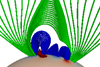 |
Fig. 1. Magnetic field configuration used as the initial condition in all the MHD simulations. Red lines represent the flux rope, blue lines the arcades, and green lines the external magnetic field. The lower boundary is colored according to the polarity of the magnetic field from blue (negative) to red (positive) in arbitrary units. |
In the initial condition, the flux rope is modeled to be colder and denser than its surroundings and when the system is allowed to evolve, the flux rope is ejected and this leads to the displacement of plasma and magnetic flux. In order to carry out this work, we have interpolated the spherical MHD domain into a cartesian box (x, y, z) where the origin is placed in the center of the Sun and the z is the line-of-sight (LOS) direction with z = 0 being the plane of sky (POS). The initial domain is rotated to have the initial position of the magnetic flux rope near the POS.
Figure 2 shows the simulation after about 23 minutes of evolution for both the column density (Fig. 2a) and the density-weighted temperature along the LOS, TLOS (Fig. 2b)
 (7)
(7)
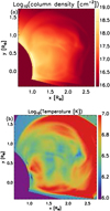 |
Fig. 2. Panel a: map of column density and panel b: map of temperature averaged over plasma density of the simulation at t = 23 min interpolated in a cartesian frame. We only show the field of view over 1 R⊙. |
The flux ejection leads to plasma traveling outwards and a structure resembling a CME, where a dense front is followed by a denser core. The same pattern is reproduced in the temperature map, where we find that the front of the ejection is hot due to the compression and is followed by a colder region that is the remainder of the ejected cold flux rope. We refer to Pagano et al. (2014) for more details on the evolution of the flux rope ejection.
2.2. Synthetic data
The spherical 3D parametric description of the CME evolution obtained by MHD simulation is interpolated onto Cartesian grid as described by Pagano et al. (2015), then from each simulated plasma element we compute the white-light total (tB) and polarized (pB) brightnesses, and the UV H I Ly-α spectral line emissivities. By integrating the contribution from each element along a given LOS we obtain the synthetic images of tB, pB and H I Ly-α intensities.
The MHD model provides 3D cubes of values for a full set of coronal plasma parameters, such as proton density, ρ, radial velocity, w, and temperature, T. The total and polarized visible light emission, tB and pB, are derived by computing the Thomson scattered light from a single electron in each cell, which only depends on the position with respect to the solar disk and the scattering angle (Minnaert 1930; Billings 1966), and then multiplied by the electron number density of each cell. From the simulated proton density ρ we compute the proton number density np = ρ/mp, where mp is the proton mass, and the electron number density, ne, from np/ne=0.83, which is a valid approximation in the typical coronal plasma condition of fully ionized atoms with He abundance equal to 10%.
In the UV spectral range the main physical processes contributing to H I Ly-α emission from an optically thin corona are the collisional excitation and the photo-excitation of the neutral hydrogen atoms, whereas the other mechanisms, such as the Thomson scattering of solar disk radiation from free coronal electrons, dominant for the white light emission, give a negligible contribution to the UV spectral lines (e.g., Gabriel 1971). Therefore, the expected emission in the UV spectral lines from solar corona, measured in photons cm−2 s−1 sr−1, can be written as
 (8)
(8)
where jr and jc are the radiative and collisional emissivities, respectively, from each volume element, and the total intensity, Iobs , is computed by the integration of all elements along the LOS.
2.2.1. Radiative component of UV emission
According to Noci et al. (1987), the radiative emissivity due to the resonant scattering of the photospheric radiation by coronal atoms is
 (9)
(9)
where B12 is the Einstein coefficient for absorption for the considered atom transition, h is the Planck constant, λ0 is the reference wavelength of the transition, ni is the neutral hydrogen number density, p(ϕ) is a geometrical function for the scattering process (Beckers & Chipman 1974), ϕ is the angle between the direction of the incident radiation n′ and the LOS, Iex (λ − δλ) is the intensity spectrum of incident radiation from lower atmosphere, δλ is the shift of the incident profile due to the radial velocity, w, of coronal absorbing atoms in the direction n′:
 (10)
(10)
and Φ(λ, n′) is the normalized coronal absorption profile along the direction of the incident radiation. In the assumption of a Maxwellian velocity distribution of the absorbing particles, the absorption profile is Gaussian with a width, σλ(n′), given by
 (11)
(11)
where c is the light speed, kB is the Boltzmann constant, and Tn′ is the kinetic temperature along the direction of the incident radiation. In case of relatively dense CME plasma it is reasonable to assume an isotropic thermal velocity distribution, therefore Tn′ = Ti , where Ti is the ion kinetic temperature both in parallel and perpendicular direction with respect to the magnetic field. Moreover, we can also make an assumption of thermal equilibrium, and considering the same ion and electron temperature, Ti = Te = T. Finally the neutral hydrogen density, ni is determined as a function of temperature by the ionization equilibrium curves given by Del Zanna et al. (2015).
In order to obtain the total radiation emitted by resonant scattering, we integrate over the solid angle subtended by the source of exciting radiation, dω, and the product between the incident and absorption profile is integrated over the wavelength, dλ. In our computation we assumed an averaged value of the exciting radiation coming from the solar disk. In particular, for H I Ly-α we adopted the SoHO/SUMER chromospheric spectral profile observed at solar minimum in July 1996 (Lemaire et al. 2002).
2.2.2. Collisional component of UV emission
The physical mechanism producing the collisional component of an emission line in the solar corona is the excitation of a coronal atom by collision with a free electron. Following Noci et al. (1987), the collisional emissivity can be written as
 (12)
(12)
where ne is the electron density and qcoll is the collisional coefficient:
 (13)
(13)
where Te is the electron temperature, E12 is the transition energy, f12 is the transition oscillator strength, and ¯g is the Gaunt factor computed by using Mewe (1972) approximation.
From the plasma parameters obtained with the MHD simulation we compute the H I Ly-α intensity images with the above expressions and described assumptions. These images are used as input to reverse the process in order to infer the CME plasma parameters, such as density, velocity, and temperature. The comparison between the model results and the parameters computed from synthetic images, both with the same assumptions, allows us to check the reliability of the procedures to determine CME plasma physical parameters from a multi-wavelength sequence of images.
3. Resulting VL and UV synthetic images
The resulting sequence of VL and UV coronagraphic intensity images is shown in Fig. 3. In particular, this figure shows the simulated CME emission in both the VL (polarized brightness, top left) and UV (HI Ly-α, top right) channels during the propagation phase. The comparison between the VL and UV images shows many interesting features that will likely also characterize future real CME observations by the Metis coronagraph. First of all, the appearance of the CME front in the two channels is completely different: while the VL channel (Fig. 3, left) shows the classical arch-shaped, bright expanding front, the UV channel (Fig. 3, right) shows the expansion of a dark arch-shaped area, spatially coincident with the VL front. Therefore, the CME front in the UV Ly-α will appear as a relative reduction of coronal emission. This difference between VL and UV is mainly (but not entirely) due to the Doppler dimming effect: because the CME front corresponds to plasma expanding with the larger radial component of velocity (with respect to the rest of the erupting plasma), the reduction in the emitted Ly-α radiative intensity will be significant. Moreover, for the CME simulated here, plasma temperatures at the front are significantly larger with respect to the rest of CME body, and this results in a reduced number density of neutral H atoms, and thus reduced Ly-α radiative and collisional emissions.
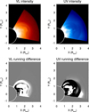 |
Fig. 3. Top panels: resulting simulated intensities of a CME in coronagraphic images acquired in the VL (left) and UV Ly-α (right) channels. Bottom panels: corresponding running differences in the two channels. |
In particular, because the radiative emission is usually dominant over the collisional one, we expect that for any CME whose front is expanding faster than ∼300 km s−1, the UV Ly-α emission from the front will be almost negligible: the front will be almost transparent in the UV. This means quite interestingly that the UV emission detected at pixels with LOS crossing the expanding front will be almost entirely due to the external corona, and not to the CME plasma. This results in a very different appearance for the so-called running difference images (shown in Fig. 3, bottom panels), where the intensities observed in the previous frame are subtracted. While the VL running difference image shows the standard brightening in pixels where the CME front and core are located, the UV Ly-α running difference images show a significant dimming at the CME front. Therefore, comparison with the pre-CME UV intensities observed at the same pixels could provide the amount of UV coronal emission removed by the transit of the CME. This latter quantity will depend on the extension of the eruption along the LOS in each pixel: the possibility to use this UV dimming to derive 3D information on the eruption will be further investigated in the future.
Figure 3 (top panels) also shows that, contrary to what happens for the CME front, the inner part of the CME appears relatively much brighter in the UV Ly-α emission with respect to the VL images, making the CME core bright even in the UV running difference (bottom panel). This is due to a combination of density and temperature effects, because the inner part of the CME is made up of a much denser and also cooler plasma. In the CME core in fact the Ly-α collisional component (roughly proportional to ne2) is dominant over the radiative component (roughly proportional to ne), making the CME core relatively much brighter in the UV, while in the VL (roughly proportional to ne) the core is only slightly brighter than the rest of the CME body. Moreover, while the VL emission is not sensitive to the temperature, the UV Ly-α emission is further enhanced in the core where the plasma is at a lower temperature, leading to a larger fraction of neutral H atoms with respect to the rest of the CME body.
This interesting result from the synthetic UV Ly-α data is better shown in Fig. 4, providing the collisional (left panel) and the radiative (middle panel) components of this line for the same frame selected for Fig. 3; the two components are shown with the same logarithmic color scale for a direct comparison. This figure shows that in the inner part of the CME the Ly-α collisional component will be dominant, while in the CME front the Ly-α emission will be very low in both the collisional and radiative components. This is totally different from what happens usually in the stationary solar corona, where the Ly-α emission is almost entirely due to the radiative excitation alone, and the collisional component is negligible. This difference between the CME front and the core is also due to the fact that in the CME front the plasma has the largest value of radial speed (if compared with the rest of the CME body), hence the most severe Doppler dimming effect. As a consequence, the ratio between the collisional and radiative components (Fig. 4, right panel) peaks at the CME core.
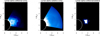 |
Fig. 4. Comparison between the collisional (left panel) and the radiative (middle panel) Ly-α components emitted by the CME and the surrounding corona; the two panels have the same logarithmic color scale going from 103 to 1011 phot cm−2 s−1 sr−1 . Right panel: ratio between the collisional and the radiative components (color scale from 0 to 5). |
The above differences in the distribution of Ly-α radiative and collisional components within the body of a CME have never been pointed out before, and will affect the possible capabilities to measure the CME plasma temperature by combining UV and VL images. In principle, given the observed Ly-α emission, and an estimate for the electron density and the radial speed of the emitting plasma, the electron temperature could be determined both by assuming that the Ly-α intensity is entirely due to collisional excitation or is due to radiative excitation alone. On the other hand, the determination of electron temperature will be much more difficult for CME regions where a mixture of radiative and collisional components is present. These difficulties are analyzed and discussed in the following paragraphs.
4. Uncertainties on the determination of CME electron densities
A key parameter for the study of CMEs is the electron density of the propagating plasma. A VL coronagraph provides images of total emission and its polarized component in a matrix of pixels that correspond to different LOS. Because of the optical thinness of the solar corona, this information is not sufficient to unambiguously determine the emitting plasma electron density distribution along the LOS. We illustrate here how to find an estimate of the width of the distribution of the electron density along the LOS, and therefore a measure of the CME electron density from the measured column density.
Assuming that the VL emission is due to Thomson-scattering of photospheric radiation, the column density can be derived for each LOS under the assumption that all the emitting plasma is located in one place along the LOS. Here, many authors in the literature usually assume that all the plasma is located on the POS (referred to here as the POS approximation), dividing the observed excess brightness by the brightness of a single electron assumed to be lying on the POS (see Vourlidas et al. 2000). Nevertheless, in a previous work (Bemporad & Pagano 2015)we have shown with numerical simulations that it is also possible to derive a better estimate of the column density by using the location along the LOS as derived with the polarisation ratio technique (referred to here as the LOS approximation), which corresponds to the center of mass of the plasma LOS distribution. Once a point along the LOS is defined, it is straight forward to compute the column density from the Thomson scattering formula. Pagano et al. (2015) have shown that the measurement of the column density is sensibly more accurate if combined with results from the polarisation ratio technique. Figure 5 shows this result for our specific case, where the relative error is displayed under the two assumptions. We define the relative error in the column density, cNe, as
 (14)
(14)
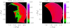 |
Fig. 5. Relative errors cNe in the determination of the column densities Ne by assuming that the whole emitting plasma is located on the POS (POS assumption, left panel) and that the whole emitting plasma is located pixel-by-pixel at the LOS position inferred from polarization ratio technique (POS assumption, right panel). |
where Ne (VL) is the column density (cm−2) computed from the inversion of synthetic VL 2D images, and Ne (MHD) is the input column density of the 3D MHD simulation. Figures 5a and b show the relative errors for the POS and LOS assumptions, respectively, with the same color scale, as derived for the CME simulation described here. We find that with the LOS approximation, the column density is measured with an accuracy of about 1%, that is, between three and four times better than what is derived with the POS approximation, as already addressed in Pagano et al. (2015). This is very important because the CME electron number density ne (cm−3) is almost always derived starting from the measured column density Ne (cm−2).
In order to derive ne from the measured Ne, it is necessary to retrieve information on the spatial distribution of the plasma density along the LOS, and in particular to estimate the average extension along the LOS L (cm) of the emitting plasma, so that ne = Ne/L. Many authors in the literature usually assume the same constant L value throughout the whole CME excess brightness image (see e.g., Ontiveros & Vourlidas 2009). On the other hand, as showed by Susino et al. (2014), this can be done alternatively from the position along the LOS of the emitting plasma as derived with polarization ratio technique for each pixel on the image. This corresponds to an assumption that variations of LOS positions in the neighboring pixels are representative of the LOS extension of plasma emission for the considered pixel. Figure 6a shows the width of the distribution computed using the formula in Susino et al. (2014) in our image.
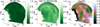 |
Fig. 6. Extension of the plasma density distribution along the LOS as derived from the analysis of VL synthetic data (left panel), and corresponding standard deviation from the center of mass for the density distribution along the LOS in our MHD simulation (middle panel). The ratio between these two quantities (right panel) shows that the LOS extension of CME plasma is underestimated by about one order of magnitude. |
However, this turns out to be an underestimate of the actual width of the plasma distribution along the LOS. Figure 6b shows the standard deviation from the center of mass for the density distribution along the LOS in our MHD simulation, and Fig. 6c shows the ratio between the values in Figs. 6b and a. We find that the actual plasma density distribution width is about one order of magnitude larger than the one measured from the mere variation of the position along the LOS. This discrepancy can be attributed to the fact that location along the LOS is already a quantity averaged on the plasma density and is therefore more stable against fluctuations on the plasma density itself.
Finally, we can apply these considerations to our study and use the synthetic visible light images and synthetic polarized component to find the electron number density for each pixel, by combining column density and the width of the plasma density distribution. Figure 7 shows the CME plasma density that we obtain by dividing, pixel by pixel, the CME column density by the width of the plasma density distribution obtained with the technique in Susino et al. (2014) and increased by one order of magnitude.
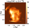 |
Fig. 7. Map of CME electron number densities as derived from the analysis of VL synthetic data (see text). |
5. Uncertainties on the determination of CME kinematic
A correct determination of the CME kinematical properties is of fundamental importance for a correct analysis of the UV Ly-α images of CMEs. This can be understood quite easily: as mentioned above, the radiative component of Ly-α emission (usually dominant in the solar corona) depends significantly on the radial component of plasma speed. Nevertheless, a CME has not a single speed, but each LOS intercepts plasma cells expanding with different speeds, and in principle the analysis should take into account, for each pixel, the distribution of velocities all along the LOS. Nevertheless, because VL and UV coronagraphic images are integrated along the LOS, and because plasma embedded in a CME does not have a simple geometrical configuration of flow-lines, as could be expected for example in polar coronal holes, it is not possible in principle to make any realistic assumption on the magnetic field configuration and velocity distribution along the LOS. Some assumptions are therefore needed in the analysis.
Because CME images are 2D, a possible approach would be for example to derive the speeds projected on the POS for all identifiable plasma features (such as filaments, threads, blobs, etc.), by tracking frame by frame each one of these features in the CME body as a function of time. Nevertheless, for the purposes of the analysis described here, only the radial component of the CME plasma speed is required, because this is the only component affecting the Ly-α emission via Doppler dimming effect. Moreover, in order to analyze 2D Ly-α images we need a continuous 2D map of Doppler dimming factors, something that could not be provided by tracking single CME features. Therefore, for this work we developed a different technique to derive pixel-by-pixel 2D maps of the radial speed νrad and Doppler dimming factors Dfact in each part of the CME body.
For this analysis we decided to focus only on the VL images, considering that the UV images are affected by the expansion velocity that we want to measure. As a first step, for each image we applied a radial filter in order to enhance the visibility of faint features; in particular we applied the normalizing radial graded filter (NRGF) described by Morgan et al. (2006). Second, considering that what we need is only the radial component of the plasma speed, each VL filtered image was converted from cartesian to polar coordinates. This allowed us to easily extract the distribution of filtered VL brightness for a fixed latitude along each radial direction. Third, for each latitude we extracted the radial VL intensity distribution in the considered frame, and the intensity distribution along the same radial, but in the previous frame. We then determined pixel by pixel the radial shift maximizing the cross-correlation between the signal in the actual frame extracted in a symmetric radial window (with width w by 80 pixels, corresponding to 1 R⊙) centered on the considered point, and the signal in a shifted radial window extracted in the previous frame. The shift required to maximize the cross-correlation around the considered pixel was assumed to correspond to the displacement in the same pixel, which was converted in a radial speed value given the time interval between each frame (174 s). With this technique the minimum and maximum altitudes covered in the 2D output speed map are reduced with respect to the input VL intensity images by an amount of pixels equal to the width w of the selected radial window. In particular, if w is the width of this radial window, all points located at a radial distance d < w/2 from the inner and outer edges of the image need to be excluded in this analysis. The resulting map of radial speed νrad was then reconverted from polar to cartesian coordinates.
An example of the resulting 2D radial speed maps is shown in Fig. 8 (left panel): to our knowledge, these are the first ever continuous 2D maps of radial CME speed derived from corona-graphic images. This figure clearly shows that the resulting speed image has the overall expected distribution, that is, maximum speed at the front, and speed decreasing with altitude throughout the whole CME body. Nevertheless, the speed distribution has also a certain level of inhomogeneity, due to the fact that different parts of the CME plasma are expanding with different speed. Similar radial speed inhomogeneities could be very important in the future analysis of real UV Ly-α observations of CMEs that will be provided by Metis. The right panel of Fig. 8 also shows the corresponding distribution of Ly-α Doppler dimming factors Dfact . Because a significant fraction of CME plasma is expanding faster than 300 km s−1 , the radial component will be severely Doppler dimmed (as described above), in particular at the front of the CME, as also shown in this figure. We also point out that similar inhomogeneities in the speed distribution will be very likely present also along each LOS, but there is no way to take into account this effect in the data analysis.
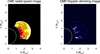 |
Fig. 8. Left panel: CME radial outflow speed map reconstructed from the analysis of synthetic VL image sequence (color scale from 0 to 1300 km s−1). Right panel: corresponding Ly-α Doppler dimming map (color scale from 0 to 5%). |
A possible improvement of the derived 2D speed maps is to also take into account 3D information derived with the polarization ratio technique and correct these maps for projection effects. Nevertheless, this has to be done carefully: the analysis of each VL pB image provides a corresponding pixel-by-pixel image for the 2D distribution of angles from the POS, θPOS , of the emitting plasma. On the other hand, a 2D speed map can only be derived by combining two VL images acquired at two different times, and the resulting speed map represents the distribution of the average radial speed between the acquisition times of the two exposures. It is therefore not possible to correct pixel-by-pixel the 2D velocity map with the corresponding pixel-by-pixel values of angles from POS, because the two maps are not representing the same plasma at the same time in each pixel. Moreover, in principle each packet of plasma in the 2D image could have a different component of velocity along the LOS, and this component cannot be measured with coronagraphic images, and can be measured only with spectrometers (from Doppler shift of spectral lines). For these reasons, the only correction that has been applied to the 2D speed maps is to assume for the whole map the same θPOS value averaged over the whole CME image. Each 2D map of the radial speed has therefore been simply divided by cos θPOS to de-project the speeds.
Once the distributions within the CME body of the electron densities and radial outflow speeds have been determined from VL images, we have all the ingredients needed for the determination of plasma temperatures combining these results with UV images. The temperature determination is discussed in the following section.
6. Uncertainties on the determination of CME electron temperatures
Before starting this section, it is very important to point out that a determination of electron temperatures only from the observed VL and UV Ly-α intensities (therefore without spectroscopic observations) has almost never been attempted. Existing measurements of CME plasma temperatures during the expansion phase are usually based on the analysis of spectroscopic data, mostly acquired by the UVCS spectrometer on-board SOHO (see Kohl et al. 2006, for a review of main UVCS results on CMEs). Therefore, thanks to the availability of spectroscopic data, electron temperatures were usually measured in CMEs with the so-called line ratio technique: considering two different spectral lines emitted with collisional excitation by two different ions of the same element, the ratio between the intensities of the two lines is dependent only on the electron temperature, which can be estimated by assuming ionization equilibrium. Alternatively, the electron temperatures have been inferred by collecting the intensities of all different spectral lines due to different ions detected by the spectrometer, and by deriving the temperature best matching the observed ionization states and the excitation rates needed to account for the observed emissions.
Nevertheless, the Solar Orbiter spacecraft does not host a UV spectrometer similar to UVCS. The only on-board spectrometer (SPICE – Spectral Imaging of the Coronal Environment) acquiring EUV spectra will not include Ly-α line in its spectral range, and will not observe the off-limb emission in the intermediate corona. On the other hand, the innovative Metis coronagraph will provide the first ever simultaneous VL and UV Ly-αimages of CMEs, but will not provide any spectroscopic information. Therefore, the test we are describing here is aimed at demonstrating how an estimate of CME electron temperatures could be derived based only on the observed images of VL and UV coronagraphic intensities, providing the first ever “CME temperature images”. To our knowledge in the literature only one similar test has been published by Susino & Bemporad (2016) based on the coronagraphic observations of three CMEs acquired in VL (SOHO/LASCO) and UV Ly-α intensities (SOHO/UVCS).
As mentioned above, the use of the UV Ly-α intensity to measure plasma temperatures has the disadvantage that the intensity of this line depends not only on the plasma electron temperature and density, but also on other parameters such as the outflow speed of the scattering atoms, their kinetic temperature, and the spatial distribution and spectral properties of chromospheric Ly-α exciting radiation. On the other hand, in contrast to other EUV filters mounted on full disk imagers in past and current space missions, the use of a narrow-band UV Ly-α filter has at least two main advantages: first, because the Ly-α is the most intense spectral line of the whole UV–EUV spectrum, there is almost no ambiguity on the atoms responsible for the observed emission. Second, because the neutral H atoms are emitting Ly-α line in a wide range of plasma temperatures, intensities measured with this filter could be used not only around a specific temperature interval (as it happens with EUV filters), but for very different plasmas going from chromospheric to coronal temperatures. This latter point makes in particular this filter very interesting for future observations of CMEs, because both chromospheric and coronal plasmas are usually embedded in the eruptions.
After this short introduction to the problem, in what follows we explain how the synthetic data have been analyzed and how the comparison with temperatures in the numerical simulation has been performed with different assumptions.
6.1. Reference CME input temperatures
In order to discuss results from the analysis, it is important to first discuss the determination of input reference temperatures. In fact, due to LOS integration, the result of any kind of analysis applied to 2D coronagraphic images will be a 2D temperature map, while the model provides us with 3D data cubes. For a comparison with output temperatures, three different input temperatures averaged along the LOS have been considered here: (1) the simple average LOS temperatures Te (LOS) = ∫z Te (z)dz/ ∫z dz, (2) the average LOS temperatures weighted by the plasma density Te (LOSn) = ∫z Te (z) ne (z)dz/ ∫z ne (z)dz, and (3) the average LOS temperatures weighted by the plasma density squared  . The resulting 2D temperature distributions shown in Fig. 9 are quite different both for the front and the core of the CME: this figure shows how the assumption made in averaging temperatures along the LOS can provide different results.
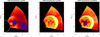 |
Fig. 9. Distribution of input CME temperatures averaged along the LOS (Te (LOS), left panel), and making an average along the LOS weighted with density (Te (LOSn), middle panel) and density squared (Te (LOSn2), right panel). In all panels the scale is Logarithmic and goes from 105.5 K (black–dark blue) up to 107.5 K (yellow–white). |
Comparison among the results in Fig. 9 shows that Te (LOS) is lower than Te (LOSn) and Te (LOSn2) almost in the whole CME body. Considering the CME core, the maximum value is given by Te (LOSn) and the minimum value by Te (LOS), while considering the CME front the maximum value is given by Te (LOSn2) and the minimum value by Te (LOS). Each one of these three input temperatures has been compared with the output temperatures derived with the three different assumptions that are described below, thus providing a 3 × 3 matrix of maps showing the relative temperature differences between the input and the output values.
6.2. Full collisional excitation assumption
The first possible hypothesis is to assume that the whole observed Ly-α emission is due to collisional excitation alone (full collisional excitation assumption – FCE). This assumption over-simplifies the estimate of the plasma temperatures, because the intensity of the Ly-α collisional component is not dependent on the plasma outflow speed, and only depends on the plasma electron density and temperature. Usually, in stationary coronal structures such as coronal streamers, the collisional component of Ly-α line is negligible, or very small. Nevertheless, the FCE assumption could be realistic for CME plasmas with higher densities and lower temperatures with respect to typical coronal plasmas, even for low outflow speeds inside the CME body. These conditions could be verified for instance in the cores of CMEs (with respect to the hotter and faster plasma embedded in the CME front), if a prominence is embedded in the CME flux rope.
Given the 2D electron density maps derived from the analysis of synthetic VL images, and the expected fraction of neutral H atoms as a function of electron temperature (by assuming ionization equilibrium), the theoretical Ly-α collisional intensity can be computed pixel by pixel as a function of temperature. A 2D electron temperature map Te (FCE) in the CME can therefore be derived from a pixel by pixel comparison between the theoretical and the synthetic Ly-α collisional intensity. An example of a resulting Te (FCE) 2D distribution for a selected time during the simulated eruption is shown in Fig. 10 (left panel). Comparison between the output temperatures derived under FCE assumption and three possible 2D distributions of input temperatures are discussed below.
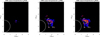 |
Fig. 10. Distribution of output CME temperatures as derived under the assumption of fully collisional Ly-α excitation (FCE; left panel), fully radiative Ly-α excitation (FRE; middle panel), and combined collisional and radiative Ly-α excitations (RCE; right panel). In all panels the scale is logarithmic and goes from 105.5 K (black–dark blue) up to 106.5 K (yellow–white). |
6.3. Full radiative excitation assumption
The second possible hypothesis is to assume that the whole observed Ly-α emission is due to radiative excitation alone (full radiative excitation assumption – FRE). This assumption is more complex than the previous one, because it requires also the derivation of a 2D outflow speed map, hence a 2D map of the Doppler dimming coefficients. This assumption could be more reliable for lower-density regions of the CME bodies (with respect to CME cores) such as the CME void, or even the CME front as long as the outflow speed and the plasma temperatures are not too large.
As for the previous case, given the 2D distribution of electron density, and by adding the 2D distribution of radial outflow speed, the theoretical Ly-α radiative intensity has been computed pixel by pixel as a function of temperature, and the plasma temperature under this second hypothesis Te (FRE) has been derived from a comparison between theoretical and synthetic Ly-α intensities. An example of a resulting Te (FRE) 2D distribution for a selected time during the simulated eruption is shown in Fig. 10 (middle panel). Comparison between the output temperatures derived under FRE assumption and three possible 2D distributions of input temperatures are also discussed below.
6.4. Radiative and collisional excitation assumption
The most complete and complex assumption is to consider at the same time both the collisional and radiative components of the Ly-α intensity (radiative and collisional excitation assumption – RCE). In this case, starting from both 2D maps of input electron densities and outflow speeds derived as explained above, the total (radiative plus collisional) Ly-α intensity is computed pixel by pixel as a function of temperature, and this latter parameter Te (RCE) is provided from a comparison between theoretical and observed synthetic intensities. An example of a resulting Te (FRE) 2D distribution for a selected time during the simulated eruption is shown in Fig. 10 (right panel). Comparison between the output temperatures derived under RCE assumption and three possible 2D distributions of input temperatures are also discussed below.
6.5. Comparison between input and output temperatures
The comparison between the input (Fig. 9) and the output (Fig. 10) temperatures derived with the different assumptions described above is shown in Fig. 11. This figure shows in particular the relative difference (normalized to the input temperatures) between output CME temperatures derived with FCE (first row), FRE (middle row), and RCE (bottom row) assumptions, and the different averages performed for input CME temperatures Te (LOS) (left column), Te (LOSn) (middle column) and Te (LOSn2) (right column). Considering that darkest (brightest) colors represent CME regions with better (worse) agreement, this relatively complex figure provides many interesting results. First of all, as a general result, all the output temperatures turn out to be underestimated with respect to the input temperatures, independent of the method considered to take into account the LOS averages. The top row in Fig. 11 shows that the FCE approximation can be used to measure the electron temperatures of CME plasma only in the denser core region, but output temperatures are always underestimated. The middle row in the same figure shows that in the CME body the FRE approximation provides a better agreement (once the radiative component has been corrected for the Doppler dimming effect; see the above discussion) with respect to the FCE approximation, and that derived temperatures match quite well simple LOS averaged temperatures (middle left panel). The bottom row in Fig. 11 shows that, overall, the best agreement is found with Te (LOSn2) temperatures only under the RCE approximation that takes into account both the radiative and collisional components. These results are discussed below.
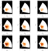 |
Fig. 11. Relative comparison between the input and the output CME temperatures (linear color scale going from 0% – black – to more than 100% – white – difference). In particular: different columns refer to the comparison between the input temperatures Te (LOS) (left column), Te (LOSn) (middle column) and Te (LOSn2) (right column) with the output temperatures derived under FCE (top row), FRE (middle row) and RCE (bottom row) hypotheses (see text for explanations). |
7. Discussion and conclusions
In this paper we faced the problem of CME plasma diagnostics using data that will be made available by future multi-channel coronagraphs. In particular, we focused on the future availability of simultaneous VL and UV Ly-α coronagraphic images that will be provided by Metis on-board Solar Orbiter, and other future similar instruments (such as LST on-board ASO-S mission). To this end, we used 3D MHD simulations to build 2D synthetic VL and UV coronagraphic images of a CME; these images have been then analyzed exploiting the full data product that will be made available by Metis, and output plasma parameters have been compared with input plasma parameters from the numerical simulation. Our main results are listed below.
-
The inversion of UV Ly-α coronagraphic images of CMEs will have a significant difference with respect to what is usually done for classical VL images. In fact, once a CME is observed in VL, the analysis usually starts from the derivation of the so-called base difference image, where the last frame acquired just before the eruption enters the telescope field-of-view is subtracted from the actual CME image. This subtraction is performed to remove the VL emission due to the coronal plasma located in surrounding regions aligned along the same LOS by also assuming that the surrounding corona is not significantly affected by the CME. This is done to isolate the emission due to the CME plasma alone, and also to remove the unknown contribution due to the F-corona. The base difference image is therefore usually employed (by neglecting pixels with negative values) to derive an estimate for the excess column density, and integrated over the whole CME body to derive the total mass of the ejected plasma. Nevertheless, it will not be possible to repeat a similar analysis with the UV Ly-α images to isolate the CME plasma emission in UV, because (as explained above) the Ly-α emission due to the denser CME plasma is not necessarily brighter than the coronal plasma existing before the eruption, because of both temperature and velocity effects. In particular, as we showed here with synthetic UV images, the CME front will be most likely dimmer than the surrounding corona. Therefore, the subtraction of background UV corona will be possible only for very limited regions of CMEs.
-
We confirmed that the derivation of the CME plasma column density and number density from the analysis of VL coronagraphic images can be significantly improved considering also the 3D information given by the polarization ratio technique. In particular, as first demonstrated by Pagano et al. (2015) with numerical simulations, a better estimate of the column density is provided by considering that the emitting plasma is located along the LOS not on the plane of the sky (as usually assumed) but on the position inferred pixel-by-pixel with the polarization ratio technique. Also, we confirmed here with the analysis of synthetic data that, as first pointed out by Susino et al. (2014) with combined VL and UV data analysis, the electron density can be derived from the measured column density not by assuming a constant value for the LOS extension of the emitting plasma (as usually assumed) but by measuring this quantity pixel-by-pixel from the distribution of LOS positions inferred with the polarization technique in the nearby pixels (see Susino et al. 2014, for more details).
-
As expected in theory, but never verified in practice before, every time the CME electron temperatures are measured from the data, it is not an easy task to identify the plasma region to which these temperatures really correspond. The plasma embedded in CME bodies is highly inhomogeneous, not only on the plane of the sky, but most importantly along the LOS. Because the CME plasma is usually optically thin both in VL and UV Ly-α (with possible exception of the prominence), the resulting intensity is due to emissions from different parcels of plasma aligned along the same LOS and – most importantly – with different plasma temperatures. In this work the output temperatures derived by assuming fully collisional (Te (FCE)), fully radiative (Te (FRE)), or a combination of radiative and collisional excitations (Te (RCE)) have been compared with the input temperatures averaged along the LOS (Te (LOS)), weighted with the density (Te (LOSn)), and with the density squared (Te (LOSn2)). As a general result, we demonstrate here that all the output temperatures turn out to be underestimated with respect to the input temperatures, whatever method is considered to take into account LOS integration effects.
-
We have shown here for the first time that sequences of CME coronagraphic images acquired in VL can be analyzed to derive 2D maps of the CME radial speed projected on the plane of the sky. To this end, successive images have been converted in polar coordinates and analyzed with a cross-correlation analysis. This result is very important for the future analyses of UV Ly-α coronagraphic images of CMEs, because it shows that it is possible to derive 2D maps of the Doppler dimming coefficients for the Ly-α emission, and therefore to derive plasma temperatures taking into account not only the collisional, but also the radiative excitation process of H atoms (usually dominant for stationary solar wind coronal plasma). Moreover, the derivation of 2D maps of CME speed can provide (in combination with 2D density maps) the first ever 2D maps of CME kinetic energies, usually overestimated by simply assuming the same (front) speed to hold for the whole CME body (see e.g. Feng et al. 2015).
-
We find that the level of agreement between the input and output temperatures depends on the considered part of the CME, on the considered average along the LOS of input temperatures, and on the considered approximation to retrieve output temperatures. In the CME core the FCE approximation is relatively good, and the LOS averaged temperatures are relatively well reproduced (within ∼60%), while temperatures in the CME body are affected by much larger errors (> 80%). The FCE approximation can also be considered as good for all the CME parts expanding much faster than ∼300 km s−1 , because at these speeds the UV Ly-α radiative component will be entirely washed out, and the observed emission will be entirely due to collisional excitation alone. Moreover, the FCE approximation is the quicker strategy, because it does not require the determination of the CME radial speed 2D map to apply the Doppler dimming correction to the Ly-α radiative component. On the other hand, temperatures derived in the CME body (excluding the projected location of the CME core) with FRE and RCE approximations are in much better agreement with the input temperatures, but the output temperature 2D maps are also affected by artificial discontinuities due to errors in the derivation of 2D maps of radial speeds. Therefore, for the analysis of real data the correct derivation of these maps will be crucial.
Temperatures derived with the FRE and RCE approximations in the CME body are in relatively good agreement with Te (LOS) (within ∼40− 50%). Poorer agreement is seen however with Te (LOSn2) (∼ 60− 70%) and Te (LOSn) (∼ 80− 90%), although in the CME core these temperatures are incorrect by factors of approximately two to four. Therefore, for the central and denser parts of CMEs, we strongly advocate deriving the plasma temperatures with the FCE approximation, which is simpler and also provides more reliable results, while for the rest of the CME the RCE approximation works much better. For the CME front where (in this simulation) the plasma temperatures exceeded 10 MK, none of the three methods give reliable temperature measurements. The reason is that in the front of the CME simulated here the plasma is so hot that the fraction of the neutral H atoms is reduced by more than one order of magnitude with respect to the typical ∼1 MK coronal plasma; moreover, because the front is the faster part of the CME, here the UV Ly-α emission is severely Doppler dimmed. The combination of these two effects made it very difficult to determine the temperatures in the front of the CME simulated here. More generally, this tells us that the combined analysis of VL and UV Ly-α coronagraphic images discussed here cannot be applied to measure such large plasma temperatures (∼ 10 MK) for parcels of plasma embedded in the CME body and expanding radially outward faster than ∼ 300 km s−1.
All the results presented here have been derived by assuming that the hypothesis of ionization equilibrium holds in the erupting plasma at any time. Because the same assumption has been considered valid both for the derivation of the synthetic UV Ly-α emissions and UV images on the one hand, and consistently for the inversion of synthetic data to derive plasma temperatures on the other, this assumption is not affecting the derived output temperatures and the comparison with the input temperatures from the MHD model. Nevertheless, the validity of this assumption during the expansion of solar eruptions is at least questionable, and has never been tested with numerical simulations. This test will be performed in a future study together with the identification of possible regions in CMEs where, as a first approximation, the hypothesis of ionization equilibrium is valid or is broken.
As mentioned above, the electron temperatures of CME plasma have been derived so far by using spectroscopic data; the use of these data has the clear and unique advantage that selecting the intensities of specific spectral lines emitted by specific ions allows for relatively precise determination of electron temperatures. Nevertheless, these data have also a very important limitation: the field-of-view of any spectrometer is limited to the 1D slit length. This limitation is acceptable for the study of stationary coronal structures such as coronal streamers, plumes, and coronal holes, and has been compensated by acquiring spectra of the same coronal features at different heliocentric distances. On the other hand, due to the rapid evolution of CMEs, these phenomena have always been observed during sit-and-stare observations, thus mixing the temporal and the spatial evolution of CME plasma parameters. In particular, for CME temperatures, the main consequence of this limitation is the actual missing knowledge of how temperatures in the expanding CME body are distributed and how they evolve as the eruption expands in the intermediate corona.
On the other hand, the techniques described here, once validated with real data and despite the existing limitations with the data analysis we discussed, could provide the first ever 2D maps of CME temperatures at different times. This will open a totally new capability of “CME temperature imaging”, allowing to study how the plasma embedded in solar eruptions is undergoing heating or cooling due to different physical processes occurring in different parts of CMEs during their expansion. Therefore, successfully applying the techniques described here to the future coronagraphic VL and UV Ly-α observations of CMEs acquired by Metis on-board Solar Orbiter and other similar instruments would provide an unprecedented view of solar eruption evolution in the intermediate corona.
Available online at solar.oato.inaf.it/UVCS_CME/index.html
Acknowledgments
This research has received funding from the European Research Council (ERC) under the European Union’s Horizon 2020 research and innovation program (grant agreement No. 647214). This work used the DiRAC Data Centric system at Durham University, operated by the Institute for Computational Cosmology on behalf of the STFC DiRAC HPC Facility (www.dirac.ac.uk). This equipment was funded by a BIS National E-infrastructure capital grant ST/K00042X/1, STFC capital grant ST/K00087X/1, DiRAC Operations grant ST/K003267/1 and Durham University. DiRAC is part of the National E-Infrastructure. We acknowledge the use of the open source (gitorious.org/amrvac) MPI-AMRVAC software, relying on coding efforts from C. Xia, O. Porth, R. Keppens.
References
- Akmal, A., Raymond, J. C., Vourlidas, A., et al. 2001, ApJ, 553, 922 [NASA ADS] [CrossRef] [Google Scholar]
- Antonucci, E., Fineschi, S., Naletto, G., et al. 2012, Proc. SPIE, 8443, 844309 [CrossRef] [Google Scholar]
- Beckers, J. M., & Chipman, E. 1974, Sol. Phys., 34, 151 [NASA ADS] [CrossRef] [Google Scholar]
- Bemporad, A., & Mancuso, S. 2010, ApJ, 720, 130 [NASA ADS] [CrossRef] [Google Scholar]
- Bemporad, A., & Pagano, P. 2015, A&A, 576, A93 [NASA ADS] [CrossRef] [EDP Sciences] [Google Scholar]
- Bemporad, A., Raymond, J., Poletto, G., & Romoli, M. 2007, ApJ, 655, 576 [NASA ADS] [CrossRef] [Google Scholar]
- Billings, D. E. 1966, A Guide to the Solar Corona (New York: Academic Press) [Google Scholar]
- Ciaravella, A., Raymond, J. C., van Ballegooijen, A., et al. 2003, ApJ, 597, 1118 [NASA ADS] [CrossRef] [Google Scholar]
- Ciaravella, A., Raymond, J. C., & Kahler, S. W. 2006, ApJ, 652, 774 [NASA ADS] [CrossRef] [Google Scholar]
- Colaninno, R. C., & Vourlidas, A. 2009, ApJ, 698, 852 [Google Scholar]
- Colgan, J., Abdallah, Jr., J., Sherrill, M. E., et al. 2008, ApJ, 689, 585 [NASA ADS] [CrossRef] [Google Scholar]
- Del Zanna, G., Dere, K. P., Young, P. R., Landi, E., & Mason, H. E. 2015, A&A, 582, A56 [NASA ADS] [CrossRef] [EDP Sciences] [Google Scholar]
- Dierckxsens, M., Tziotziou, K., Dalla, S., et al. 2015, Sol. Phys., 290, 841 [NASA ADS] [CrossRef] [Google Scholar]
- Feng, L., Inhester, B., & Gan, W. 2015, ApJ, 805, 113 [NASA ADS] [CrossRef] [Google Scholar]
- Fineschi, S., Antonucci, E., Naletto, G., et al. 2012, Proc. SPIE, 8443, 84433H [CrossRef] [Google Scholar]
- Gabriel, A. H. 1971, Sol. Phys., 21, 392 [NASA ADS] [CrossRef] [Google Scholar]
- Gilbert, H. R., Holzer, T. E., Burkepile, J. T., & Hundhausen, A. J. 2000, ApJ, 537, 503 [NASA ADS] [CrossRef] [Google Scholar]
- Giordano, S., Ciaravella, A., Raymond, J. C., Ko, Y.-K., & Suleiman, R. 2013, J. Geophys. Res., 118, 967 [NASA ADS] [CrossRef] [Google Scholar]
- Gopalswamy, N., & Yashiro, S. 2011, ApJ, 736, L17 [Google Scholar]
- Gopalswamy, N., Yashiro, S., Michałek, G., et al. 2002, ApJ, 572, L103 [NASA ADS] [CrossRef] [Google Scholar]
- Heinzel, P., Susino, R., Jejčič, S., Bemporad, A., & Anzer, U. 2016, A&A, 589, A128 [NASA ADS] [CrossRef] [EDP Sciences] [Google Scholar]
- Jejčič, S., Susino, R., Heinzel, P., et al. 2017, A&A, 607, A80 [NASA ADS] [CrossRef] [EDP Sciences] [Google Scholar]
- Kim, R.-S., Cho, K.-S., Moon, Y.-J., et al. 2005, J. Geophys. Res., 110, A11104 [NASA ADS] [CrossRef] [Google Scholar]
- Kohl, J. L., Esser, R., Gardner, L. D., et al. 1995, Sol. Phys., 162, 313 [NASA ADS] [CrossRef] [Google Scholar]
- Kohl, J. L., Noci, G., Cranmer, S. R., & Raymond, J. C. 2006, A&ARv, 13, 31 [NASA ADS] [CrossRef] [Google Scholar]
- Lee, J.-Y., Raymond, J. C., Ko, Y.-K., & Kim, K.-S. 2006, ApJ, 651, 566 [NASA ADS] [CrossRef] [Google Scholar]
- Lemaire, P., Emerich, C., Vial, J. C., et al. 2002, ESA SP, 508, 219 [Google Scholar]
- Li, H. 2015, IAU General Assembly, 22, 2232958 [NASA ADS] [Google Scholar]
- Mackay, D. H., & van Ballegooijen, A. A. 2006, ApJ, 641, 577 [NASA ADS] [CrossRef] [Google Scholar]
- Mewe, R. 1972, A&A, 20, 215 [NASA ADS] [Google Scholar]
- Michałek, G., Gopalswamy, N., & Yashiro, S. 2003, ApJ, 584, 472 [NASA ADS] [CrossRef] [Google Scholar]
- Michalek, G., Gopalswamy, N., & Yashiro, S. 2007, Sol. Phys., 246, 399 [NASA ADS] [CrossRef] [Google Scholar]
- Mierla, M., Inhester, B., Antunes, A., et al. 2010, Ann. Geophys., 28, 203 [NASA ADS] [CrossRef] [Google Scholar]
- Minnaert, M. 1930, Z. Astrophys., 1, 209 [NASA ADS] [Google Scholar]
- Morgan, H., Habbal, S. R., & Woo, R. 2006, Sol. Phys., 236, 263 [NASA ADS] [CrossRef] [Google Scholar]
- Müller, D., Marsden, R. G., & St Cyr, O. C., & Gilbert, H. R., 2013, Sol. Phys., 285, 25 [NASA ADS] [CrossRef] [Google Scholar]
- Nindos, A., Aurass, H., Klein, K.-L., & Trottet, G. 2008, Sol. Phys., 253, 3 [NASA ADS] [CrossRef] [Google Scholar]
- Noci, G., Kohl, J. L., & Withbroe, G. L. 1987, ApJ, 315, 706 [NASA ADS] [CrossRef] [Google Scholar]
- Ontiveros, V., & Vourlidas, A. 2009, ApJ, 693, 267 [NASA ADS] [CrossRef] [Google Scholar]
- Pagano, P., Mackay, D. H., & Poedts, S. 2013a, A&A, 560, A38 [NASA ADS] [CrossRef] [EDP Sciences] [Google Scholar]
- Pagano, P., Mackay, D. H., & Poedts, S. 2013b, A&A, 554, A77 [NASA ADS] [CrossRef] [EDP Sciences] [Google Scholar]
- Pagano, P., Mackay, D. H., & Poedts, S. 2014, A&A, 568, A120 [NASA ADS] [CrossRef] [EDP Sciences] [Google Scholar]
- Pagano, P., Bemporad, A., & Mackay, D. H. 2015, A&A, 582, A72 [NASA ADS] [CrossRef] [EDP Sciences] [Google Scholar]
- Porth, O., Xia, C., Hendrix, T., Moschou, S. P., & Keppens, R. 2014, ApJS, 214, 4 [Google Scholar]
- Raymond, J. C., Ciaravella, A., Dobrzycka, D., et al. 2003, ApJ, 597, 1106 [NASA ADS] [CrossRef] [Google Scholar]
- Reames, D. V. 2013, Space Sci. Rev., 175, 53 [NASA ADS] [CrossRef] [Google Scholar]
- Romoli, M., Landini, F., Antonucci, E., et al. 2017, Proc. SPIE, 10563, 105631M [Google Scholar]
- Rouillard, A. P., Odstrcil, D., Sheeley, N. R., et al. 2011, ApJ, 735, 7 [Google Scholar]
- Schwenn, R., dal Lago, A., Huttunen, E., & Gonzalez, W. D., 2005, Ann. Geophys., 23, 1033 [NASA ADS] [CrossRef] [Google Scholar]
- Spitzer, L. 1962, Physics of Fully Ionized Gases, 2nd edn (New York: Interscience) [Google Scholar]
- Susino, R., & Bemporad, A. 2016, ApJ, 830, 58 [NASA ADS] [CrossRef] [Google Scholar]
- Susino, R., Bemporad, A., & Dolei, S. 2014, ApJ, 790, 25 [NASA ADS] [CrossRef] [Google Scholar]
- Temmer, M., Veronig, A. M., Kontar, E. P., Krucker, S., & Vršnak, B. 2010, ApJ, 712, 1410 [NASA ADS] [CrossRef] [Google Scholar]
- Thernisien, A., Vourlidas, A., & Howard, R. A. 2009, Sol. Phys., 256, 111 [Google Scholar]
- Vives, S., Lamy, P., Rousset, G., & Boit, J. L. 2008, Adv. Space Res., 42, 106 [NASA ADS] [CrossRef] [Google Scholar]
- Vourlidas, A., Subramanian, P., Dere, K. P., & Howard, R. A. 2000, ApJ, 534, 456 [Google Scholar]
- Vourlidas, A., Lynch, B. J., Howard, R. A., & Li, Y. 2013, Sol. Phys., 284, 179 [NASA ADS] [Google Scholar]
- Webb, D. F., & Howard, T. A. 2012, Liv. Rev. Sol. Phys., 9, 3 [Google Scholar]
- Yashiro, S., Gopalswamy, N., Michalek, G., et al. 2004, J. Geophys. Res., 109, A07105 [Google Scholar]
- Zhang, J., Dere, K. P., Howard, R. A., & Vourlidas, A. 2004, ApJ, 604, 420 [NASA ADS] [CrossRef] [Google Scholar]
All Figures
|
Fig. 1. Magnetic field configuration used as the initial condition in all the MHD simulations. Red lines represent the flux rope, blue lines the arcades, and green lines the external magnetic field. The lower boundary is colored according to the polarity of the magnetic field from blue (negative) to red (positive) in arbitrary units. |
| In the text | |
|
Fig. 2. Panel a: map of column density and panel b: map of temperature averaged over plasma density of the simulation at t = 23 min interpolated in a cartesian frame. We only show the field of view over 1 R⊙. |
| In the text | |
|
Fig. 3. Top panels: resulting simulated intensities of a CME in coronagraphic images acquired in the VL (left) and UV Ly-α (right) channels. Bottom panels: corresponding running differences in the two channels. |
| In the text | |
|
Fig. 4. Comparison between the collisional (left panel) and the radiative (middle panel) Ly-α components emitted by the CME and the surrounding corona; the two panels have the same logarithmic color scale going from 103 to 1011 phot cm−2 s−1 sr−1 . Right panel: ratio between the collisional and the radiative components (color scale from 0 to 5). |
| In the text | |
|
Fig. 5. Relative errors cNe in the determination of the column densities Ne by assuming that the whole emitting plasma is located on the POS (POS assumption, left panel) and that the whole emitting plasma is located pixel-by-pixel at the LOS position inferred from polarization ratio technique (POS assumption, right panel). |
| In the text | |
|
Fig. 6. Extension of the plasma density distribution along the LOS as derived from the analysis of VL synthetic data (left panel), and corresponding standard deviation from the center of mass for the density distribution along the LOS in our MHD simulation (middle panel). The ratio between these two quantities (right panel) shows that the LOS extension of CME plasma is underestimated by about one order of magnitude. |
| In the text | |
|
Fig. 7. Map of CME electron number densities as derived from the analysis of VL synthetic data (see text). |
| In the text | |
|
Fig. 8. Left panel: CME radial outflow speed map reconstructed from the analysis of synthetic VL image sequence (color scale from 0 to 1300 km s−1). Right panel: corresponding Ly-α Doppler dimming map (color scale from 0 to 5%). |
| In the text | |
|
Fig. 9. Distribution of input CME temperatures averaged along the LOS (Te (LOS), left panel), and making an average along the LOS weighted with density (Te (LOSn), middle panel) and density squared (Te (LOSn2), right panel). In all panels the scale is Logarithmic and goes from 105.5 K (black–dark blue) up to 107.5 K (yellow–white). |
| In the text | |
|
Fig. 10. Distribution of output CME temperatures as derived under the assumption of fully collisional Ly-α excitation (FCE; left panel), fully radiative Ly-α excitation (FRE; middle panel), and combined collisional and radiative Ly-α excitations (RCE; right panel). In all panels the scale is logarithmic and goes from 105.5 K (black–dark blue) up to 106.5 K (yellow–white). |
| In the text | |
|
Fig. 11. Relative comparison between the input and the output CME temperatures (linear color scale going from 0% – black – to more than 100% – white – difference). In particular: different columns refer to the comparison between the input temperatures Te (LOS) (left column), Te (LOSn) (middle column) and Te (LOSn2) (right column) with the output temperatures derived under FCE (top row), FRE (middle row) and RCE (bottom row) hypotheses (see text for explanations). |
| In the text | |
Current usage metrics show cumulative count of Article Views (full-text article views including HTML views, PDF and ePub downloads, according to the available data) and Abstracts Views on Vision4Press platform.
Data correspond to usage on the plateform after 2015. The current usage metrics is available 48-96 hours after online publication and is updated daily on week days.
Initial download of the metrics may take a while.